| Issue |
A&A
Volume 622, February 2019
|
|
|---|---|---|
| Article Number | A114 | |
| Number of page(s) | 22 | |
| Section | Stellar structure and evolution | |
| DOI | https://doi.org/10.1051/0004-6361/201732482 | |
| Published online | 07 February 2019 | |
Orbital and physical parameters of eclipsing binaries from the All-Sky Automated Survey catalogue
X. Three high-contrast systems with secondaries detected with IR spectroscopy⋆
1
Nicolaus Copernicus Astronomical Center, Polish Academy of Sciences, ul. Rabiańska 8, 87-100 Toruń, Poland
e-mail: This email address is being protected from spambots. You need JavaScript enabled to view it.
2
Cerro Tololo Inter-American Observatory, Casilla 603, La Serena, Chile
3
Astronomical Institute, University of Wrocław, Kopernika 11, 51-622 Wrocław, Poland
4
Okayama Astrophysical Observatory, National Astronomical Observatory of Japan, 3037-5 Honjo Kamogata, Asakuchi Okayama 719-0232, Japan
5
Instituto de Astrofísica, Pontificia Universidad Católica de Chile, Av. Vicuña Mackenna 4860, 7820436 Macul, Santiago, Chile
6
Max-Planck-Institut für Astronomie, Königstuhl 17, Heidelberg 69 117 69117, Germany
7
The Graduate University for Advanced Studies, 2-21-1 Osawa, Mitaka, Tokyo 181-8588, Japan
8
Subaru Telescope, National Astronomical Observatory of Japan, 650 North Aohoku Place, Hilo, HI 96720, USA
9
Millennium Institute of Astrophysics, Av. Vicuña Mackenna 4860, 7820436 Macul, Santiago, Chile
10
Department of Astronomy, The University of Tokyo, 7-3-1, Hongo, Bunkyo-ku, Tokyo 113-0033, Japan
11
Astrobiology Center of NINS, 2-21-1, Osawa, Mitaka, Tokyo 181-8588, Japan
12
National Astronomical Observatory of Japan, 2-21-1 Osawa, Mitaka, Tokyo 181-8588, Japan
Received:
18
December
2017
Accepted:
10
December
2018
Abstract
Aims. We present results of the combined photometric and spectroscopic analysis of three detached eclipsing binaries, the secondary components of which are not visible or are very hard to identify in the optical spectra – ASAS J052743–0359.7, ASAS J065134–2211.5, and ASAS J073507–0905.7. The first one is the known visual binary ADS 4022, and we found that it is a quadruple system composed of two spectroscopic binaries, one of which shows eclipses. None of the systems have previously been recognized as a spectroscopic binary.
Methods. We used the following telescopes/spectrographs to collect a number of high-resolution optical and IR spectra: Subaru/IRCS, CTIO-1.5 m/CHIRON, Euler/CORALIE, MPG-2.2 m/FEROS, OAO-188/HIDES, and TNG/HARPS-N. We used these data to calculate radial velocities (RVs) and later combined them with MITSuME and ASAS photometry. The Subaru/IRCS IR spectra were crucial for secure identification of the lines of the cooler components. Radial velocity measurements were made with the TODCOR technique, and RV curves were modelled with our own procedure V2FIT. Light-curve modelling was performed with JKTEBOP and PHOEBE codes. Temperatures and metallicities of two systems were estimated from spectra. For the ADS 4022 system we also used the archival WDS data and new SOAR observations in order to derive the orbit of the visual pair for the first time. Ages were estimated by comparing our results with PARSEC isochrones.
Results. The eclipsing pair ASAS J052743–0359.7 A (P = 5.27 d) is composed of a 1.03(6) M⊙, 1.03(2) R⊙ primary and a 0.60(2) M⊙, 0.59(2) R⊙ secondary. The components of the P = 21.57 d non-eclipsing pair B likely have masses in between the two eclipsing components, and both pairs are on a ∼188 yr orbit around their common centre of mass. The system ASAS J065134-2211.5 (P = 8.22 d) consists of a 0.956(12) M⊙, 0.997(4) R⊙ primary and a 0.674(5) M⊙, 0.690(7) R⊙ secondary. Finally, ASAS J073507-0905.7 (P = 1.45 d), which consists of a 1.452(34) M⊙, 1.635(12) R⊙ primary and a 0.808(13) M⊙, 0.819(11) R⊙ secondary, is likely a pre-main sequence system. In all cases secondary eclipses are total.
Key words: binaries: eclipsing / binaries: spectroscopic / binaries: visual / stars: fundamental parameters / stars: late-type / stars: pre-main sequence
Time series photometry is only available at the CDS via anonymous ftp to cdsarc.u-strasbg.fr (130.79.128.5) or via http://cdsarc.u-strasbg.fr/viz-bin/qcat?J/A+A/622/A114
© ESO 2019
1. Introduction
During recent years we have seen an increasing interest in studies of low-mass, K and M-type dwarfs, driven mainly by the exoplanet search surveys with dedicated instruments, both photometric (Burdanov et al. 2017; Wheatley et al. 2018) and spectroscopic (Quirrenbach et al. 2010; Artigau et al. 2014; Kotani et al. 2014). The goal behind such surveys is to find Earth-sized habitable planets, which are easier to detect around cool dwarfs than around F or G-type stars. However, behind each exoplanet detection and characterisation lies knowledge of the host star, and the K and M dwarfs, despite constituting about 90% of the stars of the Galaxy, are relatively poorly studied. For decades they have been known to show significant discrepancies between the observed and predicted radii and temperatures (e.g. Lacy 1977; Popper 1997; Torres & Ribas 2002; Morales et al. 2009a). Only recently have the stellar structure and evolution models started to treat the convection and activity on low-mass stars in a way that allows to reduce these inconsistencies.
Reliable tests of these models can only be done with sufficiently precise observational data: mainly masses and radii derived for components of detached eclipsing binaries (Lastennet & Valls-Gabaud 2002; Torres et al. 2010). The number of systems with sufficiently measured parameters (relative errors below 2−3%) is constantly rising, but the vast majority of them are double-K or double-M-type pairs that are relatively faint and therefore difficult to follow up spectroscopically. Only two such pairs brighter than V = 10 mag, namely YY GemV = 9.83 in Simbad; Torres & Ribas 2002) and 1SWASP J093010.78+533859.5 (V = 9.84; Koo et al. 2014), can be found in the online catalogue DEBCat (Southworth 2015)1. For another example, AK For (V = 9.13; Hełminiak et al. 2014), very good mass measurements are available, but the available radius is slightly worse (2.6−2.9%). However, three other pairs found in DEBCat: IM Vir (V = 9.57; Morales et al. 2009b), V530 Ori (V = 9.96; Torres et al. 2014), and V2154 Cyg (V = 7.83; Bright & Torres 2017), as well as another bright system, V1200 Cen (V = 8.50; Coronado et al. 2015), prove that low-mass dwarfs can be found and studied in bright binaries as companions to stars of earlier types. A large number of pairs with secondaries of even lower mass than in V1200 Cen and V530 Ori have been reported by Triaud et al. (2017) on the basis of photometric data from the Wide Angle Search for Planets (WASP; Pollacco et al. 2006) as the outcome of the Eclipsing Binaries with Low Mass (EBLM) project. However, their dynamical masses have not yet been found.
Such pairs themselves are valuable for testing stellar-evolution models. Due to their low mass ratio, components are located relatively far from each other on the HR diagram, and differ in internal structure, level of activity, and so on. Testing the models is therefore more demanding than in the case of nearly identical pairs. Low-mass-ratio pairs are also important for the theories of binary-star formation. For example, different formation models can be distinguished by different distributions of masses of secondaries, or mass ratios in binaries (Boss 1993; Bate 2000). Unfortunately, the lower ends of these distributions are still poorly sampled due to observational restrictions; cooler secondaries are many times fainter than the hotter primaries, which makes them difficult to detect directly.
In our spectroscopic survey of southern detached eclipsing binaries (DEBs) we initially focused on searching for low-mass pairs, identifying several new ones (Hełminiak & Konacki 2011; Hełminiak et al. 2011, 2012, 2014) but finding even more relatively bright, single-lined systems with F- and G-type primaries and faint secondaries not seen or very difficult to identify in the optical spectra2. We therefore started a small, low-effort program of infrared (IR) spectroscopic observations with the Subaru telescope, targetting only a few of the most northern objects in our sample. In this paper we present three examples of those important objects, each of them showing unique, interesting characteristics. We also show that IR observations of low-mass stars paired with hotter primaries can be an efficient way to obtain important stellar parameters.
2. Detection of faint secondary components
The vast majority of spectroscopic observations are done in the optical regime. Let us consider a binary composed of a 5700 K primary (solar analogue) and a 4000 K (∼0.6 M⊙) secondary, both on the main sequence. A theoretical 5-Gyr, solar metallicity isochrone predicts a magnitude difference in V of 3.53 mag, which translates into a flux ratio (secondary over primary) of l2/l1 ≃ 0.04. Meanwhile, this ratio rises to 0.1 (2.5 mag difference) in the I band, to 0.16 (2.0 mag) in J, and 0.24 (1.55 mag) in K. The secondary is, therefore, harder to detect on shorter wavelengths, especially in spectra of relatively low signal-to-noise ratio (S/N). This was the main motivation behind our IR observations. Such a situation can be seen in the aforementioned compilation of 118 single-lined spectroscopic binaries with M-type companions by Triaud et al. (2017). The authors present a table with predicted brightnesses of secondaries in V, R, J bands, which can be compared to apparent magnitudes of the primaries. On average, the flux ratio of secondary to primary (from magnitude difference) in J is 19 times larger than in V, and exceeds 60 times in single cases.
The use of IR spectroscopy to detect faint companions has been seen in the literature for a long time (Mazeh et al. 2002, 2003; Prato et al. 2002), and is still in use (Prato et al. 2018). Apart from the higher flux ratio, another advantage is that it does not require extensive, additional observations. To obtain masses of both components, one can use information derived from the previous observations in optical, that is, the orbital solution built for a single-lined spectroscopic binary (SB1). In such cases, only one or two parameters are to be found: the velocity semi-amplitude K2 of the secondary, and (optionally) the difference between systemic velocities of two components γ2 − γ1. Since the number of free parameters is low (1–2), only a few additional observations are enough to find them. For more details, see Mazeh et al. (2002).
For a pair of G+K-type stars (Teff, 1 = 5700 K, Teff, 2 = 4000 K), assuming a Poissonian distribution of the photon noise ( ), with the signal from the secondary (l2) being ten times above the noise (σ) requires a spectrum of S/N ≃ 260 in the V band, but only 75 in J. Even if we assume that IR spectrographs have in general lower efficiencies than the optical ones, we still need exposures a few times longer in V than in J to reach the same l2/σ. Adding new, high- or very-high-S/N optical observations (which can be impossible for stars as faint as V = 11 mag without easy access to a large-aperture telescope), is therefore generally more challenging than taking a few spectra in IR.
There are advanced methods to extract the information about the faint secondary (its RVs or atmospheric parameters) from single composite spectra, or time series thereof. The Two-Dimensional Cross-Correlation technique (TODCOR; Zucker & Mazeh 1994) compares the observed spectrum of an SB2 with two template spectra, and looks for the maximum of a 2D cross-correlation function (CCF) in a v1/v2 plane, where v1 and v2 are the RVs of the primary and secondary components, respectively. It works relatively well when the difference between v1 and v2 is small (lines of both may components overlap), and does not require a high S/N. With a proper selection of templates, RV measurements of a faint secondary are possible (which was done for some of the spectra in this study). These possibilities are however limited, and a maximum of the CCF coming from the secondary can be easily confused with side peaks, which arise from coincidence of lines in the observed spectrum with different lines in the template, or simply the noise. The “proper” value of v2 may not be known without additional information.
Tkachenko et al. (2013) introduced a method of denoising the spectra on the basis of modified least-squares deconvolution (LSD; Donati et al. 1997; Kochukov et al. 2010). They show significant improvement of the S/N (by up to ten times) on single- and double-star spectra, whose initial S/N was down to 35 (for synthetic spectra) or 50 (for real observations). The undoubtful advantage is that the S/N is improved without loosing important information (e.g. line depths and asymmetries), so an analysis to obtain atmospheric parameters can be run. The LSD has been successfully applied to measure the RVs of both stars in a large-contrast binary on multiple occasions, but specific exceptions are known in the literature (e.g. KIC 5640750 in Themeßl et al. 2018). Some prior knowledge, or good assumptions of the atmospheric parameters (i.e. Teff, log(g)) are also required.
Finally, there is a variety of techniques that allow to obtain spectra of two components separately. They have their basis, for example, in disentangling the wavelength domain (Simon & Sturm 1994) or Fourier transform (Hadrava 1995), or tomographic decomposition (Bagnuolo & Gies 1991; Konacki et al. 2010). They require multiple observations that cover various orbital phases (different RV shifts), and spectra of at least moderate S/N. They also work best on homogeneous samples, meaning spectra taken with the same instrument under the same setting. Since the resulting spectrum is obtained from a combination of N spectra, the gain in its S/N is of the order of  . This means that to really improve the S/N, N must be quite large (tens of spectra). This, in practice, requires a significant amount of telescope time dedicated for observations of a given target. Without a sufficient number of quality observations, the disentangled spectrum of a faint secondary may still have its S/N too low for the purpose of further analysis (Debosscher et al. 2013; Themeßl et al. 2018).
Different approaches and different realisations of LSD or disentangling have their own advantages and limitations. For example, while some of these methods require prior knowledge of the RVs, or at least the orbital parameters, others may give the complete orbital solution without RVs as the input. There are cases that are limited to only two components, but other approaches have been shown to successfully decompose spectra of up to five stars in a system. Nonetheless, they are useful to obtain separate spectra of fainter components with improved S/N, which can be used for spectroscopic analysis, and were successfully used in multiple studies.
In our spectroscopic survey we observed nearly 300 southern DEBs, using a variety of telescopes and spectrographs, mainly of a 1–2-m class. The brightness of our targets in V varies from ∼8.5 to ∼11.5 mag, and even >12 mag in a few cases (Hełminiak et al. 2011). The survey required a substantial amount of telescope time, and optimisation of the observing strategy for the most important immediate objective: calculation of radial velocities and masses for a large number of targets. This can be effectively done with TODCOR on spectra of S/N as low as ∼20, or even lower when a stable instrument is used. Therefore, for many cases we did not attempt to obtain a large number of very-high-S/N spectra of specific targets, especially with the smaller telescopes. Moreover, for a given system, the spectra are usually collected with a few spectrographs, so the data are inhomogeneous. This is why, for large contrast objects from our survey like those described in this study, we believe that the IR observations, with the aid of TODCOR for RV calculations, provide the safest and most convenient approach, as they are direct, robust, and they consume the least telescope time (although we are considering implementation of the modified LSD for our research in the nearby future). The direct comparison of our approach with other, previously mentioned ones (LSD, spectral decomposition) is out of the scope of this paper.
3. Objects
The three presented targets were monitored spectroscopically as a part of our ongoing program of high-resolution observations of DEBs selected from the ASAS Catalog of Variable Stars (ACVS; Pojmański 2002), which is a product of the All-Sky Automated Survey (ASAS). All of them have been discovered as eclipsing binaries by the ASAS, and none of them have been recognised as a spectroscopic binary till now. This is the first study of these three systems.
ASAS J052743–0359.7 (HD 35883, TYC 4751-298-1, WDS J05278–0400AB, ADS 4022 AB, hereafter ASAS-052) is a system with V = 9.50 mag, with 0.3 mag deep primary eclipse and the secondary minimum almost invisible in the ASAS data. It is associated with the X-ray source 1RXS J052742.1–035947 (Voges et al. 1999) and has been known as a visual binary since 1902 (Aitken 1903). The Washington Double Star catalogue (WDS; Mason et al. 2001) currently gives 18 measurements of separation and position angle, some of them with the magnitudes of the components or their difference. The first 13 come from years 1902–1978 and were the only measurements known at the time of Subaru/IRCS observations. Further speckle interferometric observations with SOAR were carried out for this study. Kharchenko & Roeser (2009) gives a somewhat uncertain parallax of 21.4 ± 19.0 mas, probably affected by the binarity of the object. There is no parallax given in the Gaia Data Release 2 (GDR2; Gaia Collaboration 2016, 2018), but the catalogue lists the effective temperature of  K. We immediately noticed three sets of lines in the spectra, but only after several spectroscopic observations did we realise that the system is not triple but quadruple. Only the strongest set of lines follows the photometric period (P ≃ 5.27 d), and the other two were undoubtedly coming from the same SB2 of an unknown period. We failed to identify the second set of DEB components before the IR observations.
ASAS J065134–2211.5 (BD-22 1566, PPM 251128, TYC 5962-2159-1, hereafter ASAS-065) is the longest-period system in this study (P ≃ 8.22 d), and the faintest (V = 9.90 mag). ASAS data show a ∼0.7 mag deep primary eclipse, and almost invisible secondary. In our first optical dataset the detection of the secondary was dubious, and we failed to find it in many spectra taken later. This system is also associated with an X-ray source – 1RXS J065133.6–221121. Results of a spectroscopic analysis can be found in the fifth data release of the RAdial Velocity Experiment catalogue (RAVE; Kunder et al. 2017). The estimates of (calibrated) effective temperature (5331 ± 57 K), gravity (4.43 ± 0.08 dex), and metallicity (−0.10 ± 0.09 dex), as well as spectrophotometric parallax (12.8 ± 5.5 mas) are given. The parallax and Teff from GDR2 are formally in agreement (10.79 ± 0.03 mas and 5175 , respectively).
ASAS J073507–0905.7 (HD 60637, BD-08 1989, TYC 5397-1982-1, hereafter ASAS-073) is the brightest star in our sample (V = 9.30 mag) and has the shortest orbital period (P ≃ 1.45 d). It shows a 0.33 mag deep primary eclipse, and 0.05 mag deep secondary – deepest in the sample. As expected from such a light curve, the secondary star was more prominent in the optical spectra than in the case of the other presented system, but we were still not always able to detect it. Moreover, it is the only system for which an I-band ASAS light curve is available. On the basis of multi-band photometry Ammons et al. (2006) derived  K,
K, ![Mathematical equation: $ \mathrm{[Fe/H]}=0.01^{+16}_{-17} $](/articles/aa/full_html/2019/02/aa32482-17/aa32482-17-eq6.gif) dex, and estimated the distance to be
dex, and estimated the distance to be  pc. The GDR2 distance is, however, 171.6 ± 1.2 pc, but the effective temperature is similar:
  K.
K.
4. Observations and data reduction
4.1. Optical spectroscopy
The optical spectra were taken with a number of spectrographs that we use for our spectroscopic survey. The CHIRON spectrograph (Schwab et al. 2012; Tokovinin et al. 2013), attached to the 1.5-m telescope in CTIO (Chile), was used in “slicer” mode, which provides spectral resolution of R ∼ 90 000. This is the only telescope described here that works in service mode. Spectra were reduced with the pipeline developed at Yale University (Tokovinin et al. 2013). Wavelength calibration is based on ThAr lamp exposures taken just before the science observation. Barycentric corrections are not applied by the pipeline, and therefore we calculated them ourselves under IRAF3 with the bcvcor task. For the targets described here we did not use the “fiber” mode (more efficient but less precise than “slicer”), nor the available iodine (I2) cell. Without the I2, the stability of the instrument is estimated to be better than 15 m s−1. For the radial velocity (RV) measurements we used 36 echelle orders, spanning from 4580 to 6500 Å (limited by the templates we used), but the complete spectrum reaches 8760 Å.
The CORALIE spectrograph, attached to the 1.2-m Euler telescope in La Silla are (Chile), works in a simultaneous object-calibration mode, and provides a resolution of R ∼ 70 000. Additional ThAr exposures with both fibres are done every 1–1.5 h. For this study we used the instrument when it was still equipped with circular fibres (currently octagonal). Spectra were reduced with the dedicated python-based pipeline (Jordán et al. 2014; Brahm et al. 2017), which also performs barycentric corrections. The pipeline is optimised to derive high-precision radial velocities down to ∼5 m s−1, and reduces the spectrum to 70 rows spanning from 3840 to 6900 Å. For our purposes, we use only 45 rows (4400–6500 Å), due to the limits of our template spectra and very low signal in the blue part.
Operations at the MPG-2.2 m telescope (La Silla, Chile) with the FEROS instrument (Kaufer et al. 1999) look very similar to CORALIE, as the spectrograph also works in a simultaneous object-calibration manner, but employs an image slicer, which gives R ∼ 48 000, and the highest efficiency of all the optical instruments we used for this study (>20%), thus providing data with the highest S/N. Spectra were reduced with the CORALIE pipeline adopted to the FEROS data, capable of providing RVs with the precision of 5–8 m s−1. Although the original spectral format reaches beyond 10 000 Å, the output is reduced to 21 rows covering 4115–6519 Å, of which we use 20 (4135–6500 Å).
The three instruments described above were the main source of optical data, which were later supplemented with observations from two more facilities. The observations at Okayama Astrophysical Observatory (OAO) 1.88-m telescope in Okayama (Japan) with the HIDES spectrograph (Izumiura 1999; Kambe et al. 2013) were conducted in fibre mode with image slicer (R ∼ 50 000), without I2, and with ThAr lamp frames taken every 1–2 hours. The spectra are composed of 62 rows covering 4080–7538 Å, of which we use 30 (4365–6440 Å). Detailed description of the observing procedure, data reduction, and calibrations is presented in Hełminiak et al. (2016). The precision reached with our approach is 40–50 m s−1.
Finally, several spectra were taken with the HARPS-N spectrograph attached to the 3.6-m TNG located at the Roque de Los Muchachos Observatory in La Palma (Spain). As in CORALIE and FEROS, it also works in a simultaneous object-calibration mode. The data are reduced on-the-fly with the local Data Reduction Software, which takes care of the barycentric corrections. The product is a 1D spectrum of R ∼ 115 000 stretching from 3830 to 6900 Å. We limit our work to the 3850–6500 Å range, divided into chunks of 50 Å each.
Below we summarise the optical spectroscopic observations for each target separately.
-
ASAS-052 was observed mainly with CHIRON. Between December 2012 and December 2014, a total of 23 spectra were taken. Another 13 observations came from CORALIE, which observed ASAS-052 between November 2013 and November 2014. No marks of the secondary of the eclipsing pair were found for any of these with our approach (see Sect. 4.3), and therefore resorting to the IR was absolutely necessary for this interesting system.
-
ASAS-065 was first observed with FEROS (in March and August 2013), upon which four high-S/N spectra were secured. Three more observations, made in September and October 2013, come from CHIRON. In December 2013 we started to observe it with HARPS-N, and took six spectra by February 2015. Seven observations come from CORALIE, and were taken between March 2014 and March 2015. Uncertain marks of the secondary were found on about half of the spectra (most reliable on those coming from FEROS), but their significance was comparable to artefacts produced by TODCOR. Therefore, we decided to observe ASAS-065 in IR in order to confirm or reject these detections.
-
ASAS-073 was the first object that we observed from this sample. Six FEROS spectra were taken between November 2011 and May 2013. Later, (January 2015–January 2017) the star was re-observed with HIDES, where six more exposures were taken. On the majority (but not all) of FEROS spectra, the secondary was found rather easily compared to the two other systems, but was still somewhat doubtful. Moreover, the HIDES detections were marginal, if any detection was made at all. We treated this object as a (successful) test of the IR observations, in order to verify that the IR and optical data gave consistent results.
4.2. Subaru/IRCS infrared spectroscopy
As the optical spectra were insufficient for secure identification of the secondaries, we observed all targets in the IR. We used the 8.2-m Subaru Telescope equipped with the InfraRed Camera and Spectrograph (IRCS; Kobayashi et al. 2000) working in echelle mode, set to the J-band. With such settings the instrument produces spectra composed of nine echelle orders, stretching from 11 616 to 14 285 Å. We used the narrowest 0.14″ slit, which provides the resolution of ∼20 000. Atmospheric turbulence correction was performed with Subaru’s AO188 adaptive optics system (Hayano et al. 2008, 2010). To reduce the influence of the unstable sky background, we observed in the ABBA sequence, which is nodding along the slit. Because it was possible to resolve the two visual components of ASAS-052, we set the position angle of the slit to ∼66.4° so that the spectra of both components were recorded. In further processing we were able to extract them separately.
For the data reduction we used the standard procedures of the ccdred and echelle packages of the IRAF software. Flat-fielding was done on the basis of He lamp exposures. First a series of frames He-ON was taken and combined, followed by a series of He-OFF. Final flat was obtained by subtracting the master OFF from the master ON frame. Wavelength calibration was based initially on Ar lamp exposures taken at the beginning or end of the night, in a similar ON/OFF manner as the flats. Later, the velocity corrections were found for each science observation separately, from cross-correlation of the science spectra with a telluric standard star. Same standards were used to remove the strong telluric lines from the spectra. For the cross-correlation itself we used the task xcsao of the IRAF’s rvsao package. The barycentric time and velocity correction were calculated with the bcvcor task of the same package. Some RV standards were observed in order to monitor the stability of the instrument. Extraction of the ABBA spectra was done in a few steps. First, frames from the position B1 were subtracted from frames from the position A1 (A1 – B1 = AB1), and analogously for A2 – B2 = AB2. AB1 and AB2 were then added to get the frame AB, which was then also multiplied by −1 to get the frame BA. The “positive” spectra from AB and BA (corresponding to observations at positions A and B, respectively) were extracted with the task apal and wavelength-calibrated with refspec and dispcor, on the basis of Ar lamp frames. Location of each “positive” spectrum from AB and BA frames served as a reference for the Ar lamp extraction. Finally, the sarith task was used to add AB to BA in the wavelength domain and obtain the final spectrum.
IRCS observations took place during two nights in March and one night in December, 2014. ASAS-052 was observed four times, and in three cases the two visual components were resolved and their spectra extracted separately. Thanks to this, when the velocities were measured, it was possible to determine that component A is the eclipsing one. ASAS-065 was observed three times, and ASAS-073 only two times, as the detections of the secondary were more reliable in the high-S/N FEROS spectra than for the two other systems. In all cases, the cool components appeared much more prominent than in the optical data. However, due to a lower resolution and worse stability, the error bars of the resulting RVs of the hotter components are larger than for the optical.
4.3. Radial velocities
For the RV measurements we used our own implementation of the aforementioned TODCOR technique (Zucker & Mazeh 1994). As templates for the optical data we used synthetic spectra computed with ATLAS 9 (Kurucz 1992), which do not reach wavelengths longer than 6500 Å. For the IR observations we used synthetic spectra from the library of Coelho et al. (2005), which cover both optical and IR regions (3800–18 000 Å), but have lower resolution than the ones from ATLAS 9. This is however not a problem for IRCS, the resolution of which is approximately two to six times lower than that of the other instruments we used.
In this study we had to deal with data with one, two, or three sets of spectral features, while the TODCOR is optimised for double-lined spectroscopic binaries. If the templates are matched correctly, it also calculates the intensity ratio of the two stars. For single-line cases (many of the ASAS-065 and ASAS-073 spectra) we forced the code to look for a local maximum around a position where v1 was close to the true velocity value, and v2 was very far from it (>100 km s−1). The code looks for the maximum in each axis independently, so the resulting v1 was not affected by v2. This approach has been shown to provide satisfactory results in Hełminiak et al. (2016).
In the optical spectra, ASAS-052 appeared as either double- or triple-lined. The maximum of the CCF corresponding to the Aa component is the strongest one in this system, followed by Ba, and Bb is the weakest. Initially, the period of the Ba+Bb pair was not known, and very often one of its lines was blended with Aa, and an RV measurement was possible only for the other. Sometimes the lines of Ba and Bb were blended with each other, and we could measure the velocity of Aa. In both such cases, we treated such spectra as double-lined, but in further analyses we used only the measurement of the unblended component. When all three sets of lines were seen separately, we ran TODCOR twice: once forcing it to look around the local maximum corresponding to the positions of Ba and Bb (weaker lines), and the second time for the global maximum, corresponding to velocities of Aa and Ba (but this measurement of Ba was not taken for the orbital fit). A similar approach was successfully tested on a triple-lined system KIC 6525196 in Hełminiak et al. (2017a), where the rms of the orbital fit was comparable with the stability of the spectrograph measured from standard stars.
All but one of the IRCS spectra were double-lined, even for ASAS-052. As mentioned above, in three of four cases we could extract spectra of ASAS-052A and B separately. In the fourth case, the lines of Ba overlapped with the lines of Aa, but the features of Ab and Bb were well separated. We thus ended up with a triple-line case, and measured the velocities of Ab and Bb only.
Individual RV measurements, their errors, residuals of the fit, as well as exposure times and S/N are listed in Tables A.1–A.3.
4.4. ASAS photometry
The All-Sky Automated Survey (ASAS; Pojmański 2002) is the first source of photometry for all the targets in our spectroscopic survey. The data can be extracted from three different sites:
-
The ASAS Catalogue of Variable Stars (ACVS)4 is the catalogue of time-series photometry and identifications of the variables found by ASAS South by the third stage of the project (end of 2009). Measurements were made in the Johnson’s V band. All the studied targets have data obtained from the ACVS.
-
ASAS for SuperNovae (ASAS-SN; Shappee et al. 2014; Kochanek et al. 2017) Sky Patrol5 is part of the northern counterpart of the ASAS project. The V-band brightness measurements taken after December 2011 are available online. Many brighter objects suffer from saturation effects, and this was the main reason why in this study we used ASAS-SN data only for ASAS-052.
-
A number of bright ASAS South variables can be found in the catalogue of Sitek & Pojmański (2014)6, which contains light curves in the IC band. In this archive we only found data for ASAS-073.
We only used the points that were flagged in the archives as “good”. Each archive gives measurements of a certain object from several different cameras of a given ASAS station. To correct the systematic differences in the magnitude zero points of each camera, we first calculated average values out of the eclipses, and later shifted the data accordingly. In cases where the number of observations from one camera was very low, we excluded them all. For ASAS-052 we merged ACVS and ASAS-SN data into one light curve. We also removed obvious outliers. In total, we used 1397, 579, and 550 V-band measurements, for ASAS-052, ASAS-065, and ASAS-073, respectively, and an additional 196 IC-band points for ASAS-073.
We should also note that some photometric measurements exist in the Northern Sky Variability Survey (NSVS; Wozniak et al. 2004), but the number is low and not sufficient for light curve analysis.
4.5. MITSuME photometry
An initial analysis of the public ASAS data showed that the uncertainties of resulting parameters were very large, mainly because depths of secondary eclipses7 are comparable to the scatter of data. Problems with large uncertainties arising from such a situation are presented for example in Coronado et al. (2015) for V1200 Cen. Therefore, we decided to obtain additional photometry.
We used the Okayama station of the Multicolor Imaging Telescopes for Survey and Monstrous Explosions (MITSuME; Kotani et al. 2005) network. This observatory consists of a 0.5-m robotic telescope, equipped with a multi-band imager (Sloan g′, Cousins IC and RC) with a field of view of 26′ × 26′. Observations were made between November 2015 and April 2016 in a queue mode, with our targets scheduled in blocks of 1–2 h. Higher priority has been set for the eclipses (especially moments of entry, exit, and the minimum), and for some phases out of eclipses. Such scheduling coupled with highly unstable weather, unfortunately caused problems in covering the eclipses of ASAS-052 (P ≃ 5.27 d) and ASAS-065 (P ≃ 8.22 d), which last several hours. They are not observable in every cycle, as they often occur during the daytime. For this reason we do not have the minimum and egress of the primary eclipse of ASAS-052, and the ingress of the secondary of ASAS-065. Much shorter eclipses of ASAS-073 (P ≃ 1.45 d) are sampled sufficiently.
The CCD reduction of the raw data was done with the standard imred.ccdred routines under IRAF. Aperture photometry was done with IRAF’s apphot on the variable and several comparison stars. The object of interest was usually the brightest star in the field. For the final differential photometry we chose the comparison star that produced the smallest scatter outside of the eclipses, taking into account only frames taken under good weather conditions. If more than one comparison gave similar results, the brightest one was chosen. We later removed the obvious outliers and measurements with higher formal errors (normally taken under worse weather conditions, and producing larger scatter). Due to the shutter failure in the g′ camera we had to exclude some observations in this band. We have also decided not to use g′ data for ASAS-052 entirely, as this band suffers from the strongest systematic uncertainties, which rendered the measurements taken during the secondary eclipse useless (primary eclipses were well covered for the other two objects, so the use of g′ data was still justified). Moreover, for ASAS-052 we had no independent information on the amount of third light in g′.
The apparent magnitudes of the variable and comparison stars were obtained from the available literature sources. In case of ASAS-052 we took g′,r′, and i′ measurements from the Sloan Digital Sky Survey (SDSS) data release 12 (Alam et al. 2015), and transformed to the Cousins RC and IC magnitudes using the formulae from Jordi et al. (2006). Fields of the other two systems were not observed by the SDSS, so we used entries in the same bands from the AAVSO Photometric All Sky Survey (APASS) data release 9 (Henden et al. 2015), and the same transformations to the Cousins’ system. This procedure gave a very good match between MITSuME and ASAS IC light curves of ASAS-073.
4.6. Astrometry of ASAS-052 AB
The WDS currently contains 18 archival astrometric measurements of ASAS-052 (WDS 05278-0400), spanning 115 years (1902–2017), with a large gap between 1978 and 2015. Orbital motion of the two spectroscopic pairs around their common centre of mass can be clearly seen. During the first Subaru run (March 2014; see Fig. 1 in Hełminiak et al. 2015) we noticed that the secondary is located at a similar position angle as in 1902, which could mean that the system has almost completed one revolution since the discovery. This was confirmed by subsequent speckle interferometric and lucky imaging observations with SOAR taken in 2015 and 2017, which are summarised in Table 1. All new data are already published (Tokovinin et al. 2015, 2018), and are currently included in the WDS archive. Apart from the relative position, the magnitude difference between the two components has also been measured in three bands. They were used in the light curve analysis as starting points for the amount of third light. The observed discrepancies in Δmag between two epochs are normal for speckle data. For V and I bands we used average Δmag values, and set a conservative uncertainty of 0.1 mag for all bands.
Results of SOAR speckle observations of ASAS-052.
5. Analysis
5.1. Radial velocity curves
The model RV curves were found with the V2FIT code (Konacki et al. 2010), which fits a double-Keplerian orbit to a set of RVs of either one or two components of a spectroscopic binary by χ2 minimization with a Levenberg–Marquardt algorithm, and also deals with trends and periodic variations in the RVs of a binary. The code finds the best-fitting two semi-amplitudes K1, 2, systemic velocity of the primary γ1, difference in systemic velocities of the secondary and primary γ2 − γ1, eccentricity e, argument of periastron ω, and the time of phase zero, Tp, which is defined here either as time of periastron passage (for e > 0) or quadrature (for e = 0). If at the first run e was found to be not significantly different from zero, then another fit was made with this parameter held fixed at 0. The V2FIT can also find the orbital period, but for these systems we used values found in JKTEBOP (see following section); it can also fit offsets between measurements from two or more spectrographs, separately for each component, as they may vary with the template used for RV measurements.
Due to the fact that we have fewer RV measurements for the secondaries than for the primaries, and that they come with larger errors, we were analysing the RVs in two stages. First, each system was treated as an SB1, and only K1, γ1, e, ω and zero-point offsets between spectrographs were found from the primary’s RVs. Treating the offsets as independent variables in the fitting process is necessary to obtain correct and precise values of parameters, mainly K and, subsequently, M sin3(i), and does not introduce unnecessary sources of errors. In the second stage all these parameters were held fixed, and only K2 and γ2 − γ1 were fitted. We chose this two-step approach after running a number of initial fits comparing this manner to a single fit for all parameters from all RV data simultaneously. We noted that in complete SB2 fits the uncertainties of such parameters like e, Tp, and especially K1, are significantly larger than in SB1 fits. This is presumably due to the fact that they are influenced by RVs of the secondary, which are of worse quality than those of the primary. In the most extreeme case, the error of K1 in ASAS-052 A was about ten times larger in the SB2 fit than in SB1, leading to improbably large uncertainty in mass.
In all V2FIT runs the uncertainties were estimated using the bootstrap approach, and additionally, in the second stage (K2 and γ2 − γ1 search) a Monte-Carlo method was used to properly evaluate the influence of errors of the fixed parameters on the uncertainties of the fitted ones. In this way we took into account the possible systematic uncertainties, for example coming from the template mismatch, spots, or low numbers of spectra. We also avoid unrealistically large uncertainties coming from lower-precision data. In the case of the non-eclipsing ASAS-052 B, where both sets of lines were easily visible, and RVs of both components are comparably precise, all parameters were found simultaneously.
5.2. Modelling light curves
Due to the different characteristics of the studied objects and data sets used, the light curve analysis was slightly different for each system. Below we briefly describe the common parts, and follow with an explanation of the individual approaches.
We used two well-known and widely used light-curve-fitting codes. The first was JKTEBOP v28 (Southworth et al. 2004a,b), which is based on the EBOP program (Popper & Etzel 1981). This fast, geometrical code allowed us to assess the general characteristic of a given system, and good starting values for the second program – PHOEBE v0.31a (Prša & Zwitter 2005), which incorporates the Wilson-Deviney code (Wilson & Devinney 1971). The advantage of PHOEBE is that it works on all light curves simultaneously, and the incomplete light curves of ASAS-052 and ASAS-065 were impossible to analyse separately with JKTEBOP. At no point did we use RV measurements together with light curves. This is because neither of the two light-curve codes (the latest version of JKTEBOP works with RVs as well) allows to fit for different zero-points of various spectrographs.
Initial JKTEBOP runs were made on the ASAS V curves in order to find the orbital periods P of systems, to be used in the RV analysis (see previous section). The second JKTEBOP approach used values of mass ratio q, e, and ω found by V2FIT. In general, we fitted the mid-time of the primary eclipse T0 (time of phase zero for JKTEBOP), the sum of the fractional radii r1 + r2, their ratio k, orbital inclination i, surface-brightness ratios J, brightness scales (out-of-eclipse magnitudes in each filter) mout, and fractional amount of the third light l3, if necessary. The gravity darkening coefficients and bolometric albedos were always kept fixed at the values appropriate for stars with convective envelopes (g = 0.32, A = 0.5; Lucy 1967; Rucinski 1969). The logarithmic limb darkening (LD) law was used (Klinglesmith & Sobieski 1970) with approximate coefficients taken from the tables of van Hamme (1996). For this we assumed temperatures and gravities expected for the main sequence, solar metallicity stars of the masses found from the RVs. We verified that, for ASAS data, the uncertainty coming from using slightly inaccurate LD coefficients does not significantly influence the final errors of light-curve-based parameters.
With PHOEBE we analysed all available light curves simultaneously. We fixed the values of P, q, e, ω, γ (set arbitrarily to 0, but has no influence if RVs are not used), a (calculated from a sin(i) and i from initial JKTEBOP runs), and the effective temperature of the primary Teff, 1 (initially set to a value expected at the main sequence). The starting values of modified Kopal potentials Ω1, 2 were calculated by PHOEBE from mass ratio and fractional radii r1, 2 obtained with JKTEBOP. Starting values of several other parameters (e.g. i, l3) were also set to those found with the JKTEBOP. In PHOEBE we fitted for: zero-phase time Tph (which for eccentric orbits is different from the eclipse mid-time; see the PHOEBE Scientific Reference8), i, Ω1, Ω2, primary luminosity levels, and l3 in every band, if necessary. We also fitted for the effective temperature of the secondary Teff, 2, but in order to obtain a temperature ratio (as the assumed Teff, 1 was treated as uncertain). Limb-darkening coefficients were automatically interpolated by the code from tables of van Hamme (1996). At the last stage we fine-tuned the solutions, applying the results of spectroscopic or colour index analyses, that is, the Teff of the primary and the metallicity of the system (when applicable).
Parameter errors given directly by PHOEBE have the tendency to be underestimated. Therefore, to reliably estimate the influence of systematics, and correlations between different parameters in hyperspace, we followed the procedure of heuristic scanning suggested in Prša & Zwitter (2005). We ran a number (∼2000) of iterations, recording the output after each one, and introduced “kicks” every 50 steps, that is, we changed the current values of parameters by ten times their formal errors in a random direction. After such a kick, the fit converged to a minimum (typically after 3–5 steps), which was later evaluated using the value of the cost function λ (see: Prša & Zwitter 2005), calculated directly by PHOEBE. If several minima were found, we chose the one with the lowest λ. To evaluate the final uncertainties, we took into account results of only those iterations that ended up near the chosen minimum. For each parameter, we calculated the rms, and added it in quadrature to the formal fit error. Parameters strongly affected by systematics and degenerations typically have these rms-es larger than formal fit errors. An example of the procedure is shown in Fig. 1.
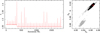 |
Fig. 1. Example of the parameter error evaluation with PHOEBE, in the case of ASAS-073. Left panel: evolution of the cost function λ. Peaks represent iterations immediately after the kicks. A more significant (deeper, λ ≃ 1.25) minimum in the parameter hyperspace was found after iteration no. 350. Right panel: mapping the degeneration between Kopal’s modified potentials Ω. The solutions included in the final error calculation are plotted with black dots, and those that were rejected (shallower minimum or still before convergence) are plotted with grey circles. The red × symbol with error bars represents the best fit (lowest λ) and the final 1σ uncertainties. |
5.2.1. ASAS-052
This system was the most difficult one to model, because of a strong third light and poor coverage of the primary eclipse in MITSuME data. For reasons explained earlier, we did not use the MITSuME g′-band observations. Initially, we kept l3 fixed to values found from SOAR observations, both in JKTEBOP and PHOEBE. The JKTEBOP fits on ASAS V-band curve favoured solutions with a total secondary eclipse. In such a situation, and having estimated l3, we could independently calculate fractional fluxes of each eclipsing component. However, while these were incorporated in PHOEBE, we could not find a satisfactory fit to all light curves simultaneously. We solved this problem after setting l3 free for the ASAS V-band under JKTEBOP. The solution we found was still showing a total secondary minimum, and predicted a slightly larger l3 in V than the SOAR observations. This can be explained with the fact that the ASAS photometric aperture and pixel scale is larger than that of MITSuME, and additional background bodies were included. With the corrected l3, V, in PHOEBE we found a satisfactory fit to all the data. Without independent information about temperatures, in later stages of the PHOEBE fit we decided to decouple the luminosities of the secondary from its temperatures. This in practice means fitting for the fluxes of the primary and secondary independently. This way we found the colour indices for the primary and used them to estimate its Teff (see sections below). Very large uncertainties of the colours of the secondary did not allow for a similar estimate for this component. Instead, we used the temperature ratio found earlier, and the colour-based Teff, 1. In the final step we fixed both values of Teff and fine-tuned the model.
5.2.2. ASAS-065
We initially thought that the eclipses were partial, but MITSuME observations showed that the shape of the well-covered primary minimum is better explained with inclination very close to 90°, when the secondary star transits close to the centre of the disk of the primary. This configuration also predicted a total secondary eclipse, but the depths of both minima could not be explained. We therefore decided to look for the third light, and found a satisfactory solution with small but measurable (several per cent) values of l3 in each band. We were fortunate to find that a small portion of MITSuME observations in the secondary eclipse was done during the total phase, which turned out to be crucial in constraining the ratios of fluxes and radii securely.
5.2.3. ASAS-073
This system was relatively easy to model. We used the largest number of light curves (five), all with very good coverage in eclipses, and sufficient coverage outside of them. No third light contribution had to be taken into account. This system also shows a total secondary eclipse (which was obvious from ASAS V data alone).
5.3. Atmospheric parameters and abundances from spectra
In ASAS-065 and -073, the primary star dominates the flux in V, so it is possible to independently assess a number of atmospheric parameters (e.g. Teff, log(g)) of the primary, and abundances of elements from optical spectra. The same cannot be done for ASAS-052 without disentangling the spectrum of Aa from the two other visible components Ba and Bb.
For the following, we used continuum-normalized FEROS spectra, shifted by the value of measured RV of the primary, stacked together, and corrected for the additional flux. Influence of additional bodies was assumed to be constant.
The effective temperature Teff, surface gravity log(g), and microturbulence ξt of the analysed stars were determined using the Balmer lines, neutral and ionised iron lines, and strong lines of Mg, Ca and Na. For both stars we used a spectrum-synthesis method relying on an efficient least-squares optimisation algorithm (see e.g. Niemczura et al. 2015, and references therein). This method allows for a simultaneous determination of various parameters that affect the shape of spectral lines, like Teff, log(g), ξt, v sin(i), and the relative abundances of the elements. Because the atmospheric parameters are correlated, Teff, log(g), and ξt were obtained prior to the chemical abundance analysis. The v sin(i) values were determined by comparing the shapes of observed metal line profiles with the computed profiles (Gray 2005).
In later steps, after Teff had been estimated for the secondaries, the influence of additional components on the atmospheric parameters of primaries was verified in the following way. First, a synthetic, continuum-normalized, “clean” spectrum of a primary was created with S/N representative for the shift-and-stacked FEROS spectra (with relative fluxes preserved). Then, a series of synthetic spectra of secondaries were created, with relative RV shifts, fluxes and S/Ns corresponding to the FEROS observations. These spectra were summed, scaled by l2/l1, and added to the “clean” spectrum of the primary to create “dirty” spectra (which mimic the true shift-and-stacked FEROS spectra used for the analysis). The atmospheric parameter search has been repeated on both “clean” and “dirty” spectra (for both ASAS-065 and ASAS-073), and results have been compared. We found out that the “clean” spectrum gives results that are indifferent from the “dirty” one, that is, differences are smaller than half the uncertainties we have adopted. As for individual lines, the depth changed by no more than 4%, and due to the varying RV difference between primaries and secondaries, the influence on abundances should be negligible. Only the strongest lines of the secondaries (which are smeared in RV in any case) could affect single lines of the primaries, but this would not have changed the overall, final results.
Chemical abundances themselves were determined from many different spectral parts. Every investigated part of the spectrum consisted of one line or many lines and blends, depending on the analysed wavelength range and the rotation velocity of the star. Line profile fitting is possible for slowly rotating stars, however for stars with medium and high v sin(i) values, spectrum synthesis on broader spectral parts is necessary. We derived the average values of individual abundances at the end of the chemical analysis.
We used atmospheric models (plane-parallel, hydrostatic and radiative equilibrium) computed with the ATLAS 9 code, and synthetic spectra calculated with the line-blanketed, local thermodynamical equilibrium code SYNTHE (Kurucz 1992; Sbordone 2005). We used the line list available at the web-site of F. Castelli9.
For ASAS-065 we used Balmer Hβ and Hα lines to find the first approximation of effective temperature. In this step log(g) = 4.0 dex, ξt = 1 km s−1 and solar metallicity were assumed as starting points. For Teff < 8000 K Balmer lines are not sensitive to the log(g). Next, the atmospheric parameters were improved through the analysis of Fe I and Fe II lines. Effective temperature was changed until there was no trend in the abundance versus excitation potential for the Fe I lines. Microturbulence was adjusted until there was no correlation between iron abundances and line depths for the Fe I lines. Surface gravity was found by requiring the same abundances from the analysis of Fe I and Fe II lines. Simultaneously, the projected rotational velocity v sin(i) was obtained. Strong lines of Na I D1 (5889.95 Å) and D2 (5895.92 Å), Ca I (6162.18 Å), and Mg I b (5183.62 Å) show strong pressure-broadened wings in the spectra of cool stars, and were used for the determination of surface gravity (Gray 2005). The uncertainty of log(g) was obtained by changing the previously found Teff and ξt in their error bars. Final atmospheric parameters, Teff = 5500 ± 100 K, log(g) = 4.4 ± 0.1, ξt = 1.0 ± 0.1 km s−1, and v sin(i) = 5.8 ± 0.4 km s−1 were used to perform a detailed analysis of chemical abundances, which is summarised in Table 2 and Fig. 2. ASAS-065 appears to be slightly more metal rich than the Sun.
Chemical abundances of ASAS-065 and ASAS-073 and their standard deviations, calculated for elements calculated from more than three spectral parts.
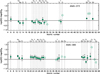 |
Fig. 2. Abundances of ASAS-073 (top panel) and ASAS-065 (bottom panel) from the detailed spectral analysis, compared to solar abundances. Open circles without error bars refer to elements for which fewer than three lines were used, hence errors were not estimated. |
The initial effective temperature of ASAS-073 was also obtained from Balmer Hβ and Hα lines, and subsequently improved by the analysis of the dependency of Fe I abundance on excitation potential. Also the microturbulence and the v sin i were determined in the same way as for ASAS-063. The determined atmospheric parameters, Teff = 6400 ± 100 K, log(g) = 4.2 ± 0.1, ξt = 1.6 ± 0.2 km s−1 and v sin(i) = 54 ± 2 km s−1 were used to perform a detailed analysis of chemical abundances (see Table 2 and Fig. 2). ASAS-073 appears to be relatively metal-poor in comparison to the Sun.
The determined microturbulence velocities for both stars are typical for stars in the observed temperature and surface gravity ranges (see e.g. Smalley 2004; Niemczura et al. 2015, 2017).
The obtained parameters are subject to errors resulting from a number of different sources, including those coming from adopted atmospheric models calculated with specific assumptions (e.g. LTE instead of full non-LTE and 1D rather than 3D approach; see Niemczura et al. 2015, for more discussion). The influence of a selected set of atomic data and their completeness must be noted. The important factors are quality and wavelength range of the analysed spectrum and its normalisation. The last parameter is particularly important for heavily blended spectra of stars with moderate or high v sin(i) values. In addition, the chemical abundance values are influenced by inaccurate atmospheric parameters Teff, log(g), and ξt. Such errors were discussed by Niemczura et al. (2015). Usually, the combined errors of chemical abundances calculated assuming ΔTeff = 100 K, Δlog(g) = 0.1, and Δξt = 0.1 km s−1 are less than 0.2 dex.
In the case of ASAS-065 we have also independently estimated Teff using line-depth ratios (LDR). This was possible thanks to low rotational velocity (narrow, unblended lines) and the absence of easily visible lines coming from the secondary or the third light. The same could not be done for ASAS-073 due to significant rotational broadening (>50 km s−1), which made the lines of interest blended, and the weaker ones unrecognisable. We chose five LDR–Teff calibrations from Kovtyukh et al. (2004), with the smallest rms (below 50 K), and used them for four FEROS and five HARPS-N spectra. The results were averaged, and the rms was adopted as the uncertainty. We obtained Teff, 1 = 5420(60) K, confirming the value obtained from Balmer and Fe lines (which was ultimately taken as the final). This agreement again shows that, in our spectral analysis, the contribution of the second (and third) light has been sufficiently accounted for, and results are reliable. Further confirmation comes from RV+LC estimates of log(g1) and velocity of synchronous rotation vsyn, 1 (see following sections), which can be compared to v sin(i). For both ASAS-065 and ASAS-073 the agreement in both parameters is better than 2σ.
5.4. Absolute parameters
The absolute values of parameters were calculated with the JKTABSDIM10 procedure, which is available with JKTEBOP. This code combines the output of spectroscopic and light curve solutions to derive a set of stellar absolute dimensions, related quantities, and distance, if effective temperatures are known or can be estimated. For distance determination, this code uses the apparent, total magnitudes of a given binary in U, B, V, R, I, J, H, K bands. For ASAS-052 and ASAS-063, we could only use estimates of apparent total brightness in V, R, and I, corrected for the influence of the third light. In the case of ASAS-073, we also used J, H, K from 2MASS (Skrutskie 2006). The code compares the observed (total) magnitudes with absolute ones, calculated using a number of bolometric corrections (Bessell et al. 1998; Code et al. 1976; Flower 1996; Girardi et al. 2002), and surface brightness-Teff relations from Kervella et al. (2004). Flux ratios may also be used to further constrain individual absolute magnitudes of each component. As the final distance value, we adopted a weighted average of all individual results given by JKTABSDIM.
Apart from stellar, photometric, and orbital parameters, JKTABSDIM also calculates the rotation velocities predicted for the case of synchronisation of rotation with orbital period vsyn, the time scale of such synchronisation τsyn, and the time scale of circularisation of the orbit τcir. The two time scales are calculated using the formalism of Zahn (1975, 1977).
5.5. Comparison with isochrones
In order to estimate the age and evolutionary status of the studied systems, we compared our results with theoretical isochrones. We made the comparison on mass ℳ versus radius R, effective temperature Teff, and luminosity L planes. We used the latest version (v1.2S) of PAdova and TRieste Stellar Evolution Code11 (PARSEC; Bressan et al. 2012; Marigo et al. 2017). The solar-scaled composition for this set follows the relation Y = 0.2485 + 1.78Z, and the solar metal content is Z⊙ = 0.0152 (Bressan et al. 2012). Whenever possible, we used our own estimates of [M/H], assuming it to be equal to [Fe/H] from the spectral analysis.
6. Results
6.1. ASAS-052
This is a rare example of a high-order (n > 3) multiple that contains an eclipsing binary. There are only several such known systems, including YY Gem, (Torres & Ribas 2002), V994 Her (Lee et al. 2008), ASAS J011328–3821.1 (Hełminiak et al. 2012), HD 86222 (Dimitrov et al. 2014), KIC 7177553 (Lehmann et al. 2016), 1SWASP J093010.78+533859.5 (Koo et al. 2014), EPIC 220204960 (Rappaport et al. 2017), V482 Per (Torres et al. 2017), KIC 4150611 (Hełminiak et al. 2017b), and EPIC 219217635 (Borkovits et al. 2018). Such systems are usually found in hierarchical configurations, meaning that their components tend to form short-period pairs, which themselves are in large separations. Such objects are interesting from the point of view of stellar formation and dynamical interactions.
Below we separately discuss our results for the eclipsing and non-eclipsing pairs, and for the “large”, astrometric orbit.
6.1.1. The eclipsing pair
In Fig. 3 we present the observed and model RVs of ASAS-052 A. The MITSuME IC, RC, and ASAS V-band photometry, with the best-fitting model light curves, are shown in Fig. 4. Orbital and physical parameters are shown in Table 3. As mentioned before, the secondary was seen only in the IR spectra. We note that this pair has the lowest flux ratio l2/l1 in all bands (0.017 in V), and the secondary is the lowest-mass star in our sample (0.604 M⊙). The low number of RV measurements (four) available for the secondary is the main reason behind the large mass errors – 5.72 and 3.31 % for the primary and secondary, respectively. This is still reasonably good, but is far from what is currently possible. Relative errors in radii are 1.85 and 3.74% for the primary and secondary, respectively, and are satisfactory, considering incomplete minima coverage. The errors in fractional radii come from the uncertainty of Kopal’s potentials Ω, which themselves were degenerated with inclination, and the mass ratio, which is embedded in Ω1, 2. These degenerations are taken into account in the adopted errors.
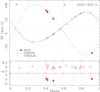 |
Fig. 3. Model RV curves (blue lines) and measurements (red points) of the eclipsing pair ASAS-052 A. Open symbols and the solid line refer to the primary, and solid symbols and the dashed line to the secondary. The dotted horizontal line marks the systemic velocity of the primary. Residuals (all in km s−1) are shown below. Symbols used for each of the instruments are labelled. The phase zero is set to the pericentre time TP. Phases of primary (P) and secondary (S) eclipses are marked with vertical dotted lines and labelled. |
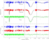 |
Fig. 4. Model light curves (white lines) and measurements (coloured points) of ASAS-052. The Y axis shows the observed magnitude, with no vertical shifts. Bands and instruments are labelled. Residuals (O − C) are shown below. For consistency, phase zero is set to the primary eclipse mid-time T0. The phase of pericentre passage is marked with a vertical dotted line and labelled “Per”. Note how the depth of the secondary eclipse changes with wavelength. |
Orbital, photometric, and absolute physical parameters of the three studied eclipsing binaries.
The primary absolutely dominates the pair A, and constitutes about 55% of the total flux of the whole quadruple system, while over 40% comes from the additional light. For this reason we did not take into account any estimates of the effective temperature found in the literature, which all assume the target is a single star. As mentioned before, we have calculated three observed colours, and used the colour–Teff calibrations from Worthey & Lee (2011). We adopt a weighted average of single Teff values predicted by each colour index. For the primary we got (V − IC)1 = 0.83(8), (V − RC)1 = 0.43(8), and (RC − IC)1 = 0.41(6) mag, which together gave 5300(340) K, assuming log(g)1 = 4.408 dex. Analogously, for the secondary we have (V − IC)2 = 2.1(9), (V − RC)2 = 0.5(9), and (RC − IC)1 = 1.50(15) mag. The errors of (V − IC) and (V − RC) are so large because the uncertainty of the secondary’s flux in V is comparable to the flux itself – 0.20(13), in PHOEBE’s arbitrary units. This error is basically the same as for the flux of the primary – 11.02(13). In cases of pairs with such a high contrast, the poor quality of ASAS photometry can even make the error larger than the contribution of the fainter star.
For the record, Teff, 2 estimated from (RC − IC), the only index that had sufficiently small formal uncertainties is 3180(120) K. The temperature of the primary from (RC − IC) only is 5170(380) K. The ratio of these two colour-based temperatures, Teff, 2/Teff, 1 = 0.62 ± 0.05, agrees within 2σ with the one obtained from PHOEBE: 0.697 ± 0.002. Both values are likely affected by the incomplete coverage of primary eclipse in MITSuME data.
The distance obtained with JKTABSDIM based on the adopted temperatures (Table 3) is 102(14) pc. No interstellar extinction has been assumed. We used the following observed magnitudes: 10.12(7) mag in V, 9.69(4) mag in RC, and 9.25(5) mag in IC. The resulting value is the weighted average of nine single estimates, and their rms is taken as the distance uncertainty. Unfortunately, this system does not have any direct parallax determination, even from GDR2, probably because it is a visual binary, so we were not able to confirm if our temperature scale is sound.
The temperatures were also crucial for the comparison with isochrones, which is shown in Fig. 5. Due to large uncertainties of Teff, and a lack of other, independent estimates of temperatures, the following results should be treated with caution.
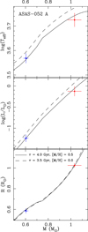 |
Fig. 5. Comparison of our results for ASAS-052 A with theoretical PARSEC isochrone for the age of 4.0 Gyr and [M/H] = +0.5 dex (solid line) and solar-composition 3.5 Gyr (dashed) on mass vs. temperature (top panel), luminosity (middle panel), and radius (bottom panel) planes. The primary is marked with the red symbol, and the secondary with blue. |
The obtained temperatures are significantly lower (by a few hundred Kelvin) than those predicted by a solar metallicity isochrone for the main sequence, which, however, still fits within 2σ. Nevertheless, we investigated the possibility that ASAS-052 is more metal rich than the Sun. A very good agreement between the model and our measurements was found for a very high value of [M/H] = 0.5 dex. The formally best-fitting isochrone of this [M/H] is for the age of 4.0 Gyr, mostly constrained by the radius of the primary. Unfortunately, relatively large mass and temperature errors do not allow for precise age determination. The system would be slightly younger, provided that [M/H] is lower. For instance, the best-fitting solar-composition model was found for the age of 3.5 Gyr. The eccentricity of the orbit is significant (0.145 ± 0.005), and the time scale of circularisation of the orbit, given in Table 3, is 1.56 Gyr, which is less than the age estimated from isochrones. The eccentricity may be, however, pumped by the presence of the component B. Our astrometric solution (see following sections) suggests that the A+B orbit is highly eccentric, and not coplanar with the eclipsing orbit.
Notably, parameters of the low-mass secondary match the 4.0 Gyr, [M/H] = 0.5 isochrone. Its radius is nicely reproduced by main-sequence models, which is not always the case for stars of such mass. The X-ray emission detected from ASAS-052 definitely shows that the system contains active stars, but we cannot say which ones are active, or even how many.
To summarise, considering the limitations of our analysis, we refrain ourselves from any conclusive statements about the exact age or metallicity of ASAS-052. We can only conclude that the [M/H] of the system is likely higher than zero, and all components are on the main sequence. The 4.0 Gyr [M/H] = 0.5 isochrone we adopted reproduces our results fairly well, especially the temperatures, but [M/H] = 0.0 models fit within errors as well. We would like to stress that we adopted this unusually high metal content only to match the obtained temperatures. It is possible that our colour-based Teff scale was affected by the reddening, which we have not taken into account. To shift the colour indices to solar metallicity values, one would have to assume E(B − V) of the order of 0.1 mag. This seems to be unlikely at a distance of ∼100 pc. To confirm (or disprove) our Teff scale, independent distance and/or reddening evaluation is required.
6.1.2. The non-eclipsing pair
The orbital parameters of ASAS-052 B, derived from the RV fit, are given in Table 4. The observed and modelled RVs are shown in Fig. 6. We reach a very good precision of 0.42% in ℳsin3i of both components. From the height of peaks in the CCF, we can deduce that brightness of Ba and Bb is somewhere between the components of A; since the system seems to reside on the main sequence, the same can be said for the masses. Moreover, fractional amounts of the third light (l3) in IC and RC (Table 3) suggest that this pair is redder, and therefore also cooler, than A. The fact that l3 is even more significant in V, and larger than the estimates from SOAR observations, may be explained by a larger photometric aperture and pixel scale of the ASAS cameras, in comparison with MITSuME – faint background sources were included in the measured flux.
Orbital parameters of ASAS-052 B from V2FIT.
We have checked the residuals of light-curve fits, and found no obvious signs of eclipses with the period of 21.5704 d. This means that the inclination of the orbit of B cannot be close to 90°. The rigid, conservative limits for the masses are therefore ⟨0.662 : 1.032⟩ and ⟨0.604 : 0.941⟩ M⊙ for Ba and Bb, respectively.
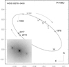 |
Fig. 7. Astrometric orbit of the ASAS-052 B relative to A (large asterisk symbol). The pre-2015 WDS measurements are shown with crosses, and the SOAR data with squares. Dates of some observations are labelled, and the orientation and direction of orbital motion is shown. The inset shows a piece of SOAR interferogram, with the same orientation as the orbit. |
We took the 4.0 Gyr isochrone for [M/H] = 0.5, and attempted to estimate the true masses by comparing the observed and predicted absolute magnitudes in V, RC, and IC. We incorporated the distance estimate from JKTEBOP, the adopted Δmag between A and B from SOAR observations (Table 1), and mass ratio from Table 4. The total absolute magnitudes of ASAS-052 B should be 5.6(3) mag in V, 5.1(3) mag in RC, and 4.6(3) mag in IC (errors include uncertainties in Δmag, distance, and observed magnitudes of pair A). We found that these total magnitudes and the given mass ratio are reproduced by a pair of 0.89(4) and 0.81(4) M⊙ stars. The inclination angle of the inner, 21.57-day orbit would thus be 69°, and no eclipses would occur.
6.1.3. Wide orbit of ASAS-052 AB
We combined the new and old astrometric measurements, and for the first time found a solution for the outer orbit of the system. These orbital parameters are presented in Table 5. The orbit is very eccentric, with a projected angular separation at pericentre of ∼33 mas, which explains the lack of astrometric observations after 1978. We used our direct determination of the total mass of A (1.638 M⊙), the indirect estimate for B (1.694 M⊙), the period of the orbit, and its projected major semi-axis â to estimate the dynamical parallax. We got 9 ± 4 mas, or 110 ± 50 pc. This is in agreement with the value calculated by JKTABSDIM. The precision is however much worse, hampered mainly by the large relative uncertainty of â.
Orbital parameters of the ASAS-052 AB system.
The current orbital solution and distance from JKTABSDIM predict that the physical separation at pericentre is as small as ∼4 AU. We can therefore expect strong gravitational interactions between two pairs, which possibly increase their eccentricities. However, for the pair A we can exclude the Mazeh–Shaham mechanism (MSM), which produces periodic eccentricity variation known as the Kozai cycles (Kozai 1962; Mazeh & Shaham 1997). In order to work, the timescale of the Kozai cycles must be shorter than the period of the pericentre precession of the inner orbit. We used the formulae given in Fabrycky & Tremaine (2007) to estimate both quantities. In case of ASAS-052 A relativistic precession is the dominant one, and its period is ∼20 000 yr. Meanwhile, the predicted Kozai cycle timescale is about 68 000 yr, so the main condition for the MSM to work is not met.
6.2. ASAS-065
The results of our analysis of ASAS-065 are presented in Table 3. Figure 8 contains the RV curves, while four light curves are shown in Fig. 9. This is the system with the best precision in mass and radius determination: 1.29 + 0.71% uncertainty on the masses of the primary and secondary, respectively, and 0.40 + 1.05% analogously for the radii. This is due to the narrowest lines (hence highest RV precision), longest orbital period, and good coverage of both minima, including the totality of the secondary. Worth noting is the fact that the rms of the RV fit of the primary from the optical spectra only is 19 m s−1, sufficient to detect massive planets on circumbinary orbits.
The contribution of the primary in V is 95% to the flux of the binary, and 85% to the total flux. The sources of the third light contamination are possibly two faint stars. One is located about 5 arcsec from the DEB, and is found in several catalogues. It was likely within the photometric aperture of ASAS. Its distance and proper motion listed in GDR2 suggest that it is gravitationally bound to ASAS-065, which makes the system a physical triple. The GDR2 gives a temperature of  K, which makes it cooler than the secondary of the eclipsing pair. The other is a visual companion, separated from ASAS-065 by only about 0.45 arcsec, which we have seen on acquisition and guiding images during our Subaru observations. Assuming that it is the only contaminant of MITSuME photometry, it appears to be bluer than the secondary and brighter in g′, but fainter in RC and IC, which suggests it is a background star. Confirmation should, however, come from dedicated adaptive optics observations.
At the beginning it was somewhat uncertain to us how the secondary or the third light(s) affect the results of spectroscopic analysis. The most recent one, from RAVE DR5 (Kunder et al. 2017), gives the calibrated Teff = 5330(60) K, [M/H] = −0.10(9) dex, and log(g) = 4.43(8) dex. The agreement with our results is within 2σ, even though this analysis does not take into account binarity or third light. We note that the RAVE spectra are taken in the I band, where the contribution from the primary to the total flux drops to 79%, and with much lower spectral resolution. This is probably the reason why Mints & Hekker (2017) underestimated the mass of ASAS-065, and obtained 0.832 M⊙, with the 3σ uncertainty range ⟨0.741 : 0.933⟩ M⊙. One can see that it is only marginally in agreement with our dynamical mass of the primary (⟨0.920 : 0.992⟩ M⊙ 3σ range; Table 3).
We used our estimates of Teff and apparent V, RC, IC magnitudes (after correction for the third light) to calculate the distance with JKTABSDIM. The nine individual values produced by the code gave the weighted average of 108(10) pc when no extinction was assumed. This is in good agreement (∼1.4σ) with GDR2, which gives 92.72(25) pc. The GDR2 value can be reached for E(B − V)∼0.12 mag.
Comparison with PARSEC isochrones for [M/H] = 0.09 dex gave the estimated age of 6.3 Gyr (Fig. 10). This age may be considered surprising for the seemingly high metal content, but one should note that the orbit is nearly circular and both components seem to rotate synchronously, despite the period of ∼8.2 d (the circularisation time scale, as estimated by JKTABSDIM, is ∼19 Gyr); the metallicity is consistent with solar within the error bars. The 6.3 Gyr isochrone matches the primary very well (within 1σ) on all three planes. This age suggests that the primary ends its main sequence evolution, and slowly moves towards the sub-giant branch. The luminosity of the secondary is also reproduced correctly, Teff is within 2σ, but its radius is not. The measured R is larger than the model, and Teff is clearly lower. This is however a common feature observed in many low-mass stars in eclipsing binaries. The most popular explanation involves stellar activity, enhanced by rapid rotation (when the star is tidally locked in a short-period binary) through some version of a dynamo mechanism. However, several well-measured systems, like V636 Cen (Clausen et al. 2009), LSPM J1112+7626 (Irwin et al. 2011), ASAS J045304–0700.4 (Hełminiak & Konacki 2011), or KOI-126 BC (Feiden et al. 2011) seem to contradict this scenario. The ASAS-065 system is an X-ray source, and we can see clear emission in cores of Ca H and K lines (in HARPS-N spectra). Therefore, we can securely claim that chromospheric activity in the system is strong, and may be the reason why the secondary is inflated, but is likely not enhanced by rotation. ASAS-065 clearly shows narrow spectral lines, the velocity of synchronous rotation of the secondary (from JKTABSDIM) is only 4.2 km s−1. Notably, a similar situation occurs in V530 Ori (P = 6.11 d, M1 + M2 = 1.004 + 0.596 M⊙; Torres et al. 2014), where authors managed to reproduce observed radii with models that assume the existence of strong magnetic fields in both components.
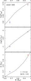 |
Fig. 10. As in Fig. 5, but for the eclipsing binary ASAS-065. The isochrone is for 6.3 Gyr and metallicity of +0.09 dex. |
Our results are precise enough to be used for reliable tests of stellar-evolution models. This system seems to be interesting from this point of view, as it is composed of a solar analogue and a low-mass star. There are only a few similar, precisely measured DEBs known, for example V1174 Ori (1.009+0.731 M⊙; Stassun et al. 2004), IM Vir (0.981+0.664 M⊙; Morales et al. 2009b), or the aforementioned V530 Ori. For the first,V1174 Ori, [M/H] has not been estimated. A few other systems, like 1SWASPJ011351.29+314909.7 (0.945+0.186 M⊙; Gómez Maqueo Chew et al. 2014), or ASAS-052 A show similar characteristics, but their parameters have not been accurately measured. The secondary is also interesting by itself, as it fills a gap in well-measured stars of masses around 0.65–0.7 M⊙. The DEBCat lists only four such objects, secondaries of ASAS J082552–1622.8 (0.687 M⊙, 0.699 R⊙; Hełminiak & Konacki 2011), V404 CMa (0.662 M⊙, 0.680 R⊙; Różyczka et al. 2009), KIC 6131659 (0.685 M⊙, 0.639 R⊙; Bass et al. 2012), and IM Vir (0.664 M⊙, 0.681 R⊙). One should also mention the primaries of AK For (0.697 M⊙, 0.687 R⊙; Hełminiak et al. 2014), and T-Cyg1-12664 (0.680 M⊙, 0.799 R⊙; Iglesias-Marzoa et al. 2017), which are not in DEBCat due to the slightly worse precision of measurements for these systems. Except KIC 6131659 B, which has a long orbital period of 17.53 d, all these stars have inflated radii, and are rotating synchronously in tidally locked configurations, although AK For A matches the theoretical isochrone within uncertainties (∼2.9% in radii).
6.3. ASAS-073
The most massive eclipsing binary in this study is composed of an F-type primary and a K-type secondary. Figure 11 shows the RV curves, five light curves are presented in Fig. 12, and the resulting parameters are listed in Table 3. Short period, circular orbit, ellipsoidal variations of the light curve, and broad spectral lines strongly suggest tidal equilibrium in this system. We obtained a relatively good precision in masses: 2.3 and 1.6% for the primary and secondary, respectively, hampered by rotationally broadened lines. Our precision in radii determination is even better: 0.72 + 1.34%, thanks to good-quality MITSuME light curves. Since no third light had to be assumed, for distance determination with JKTEBOP we could use observed total magnitudes in more bands that just the ones we observed in. We used the Teff, 1 from spectral analysis, and Teff, 2 calculated using the temperature fraction derived with PHOEBE. Our adopted distance of 170(5) pc assumes no extinction. This is an average of 16 single values, and their rms is taken as the uncertainty. It is in a very good agreement with Gaia DR2, which gives 171(2) pc.
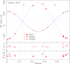 |
Fig. 11. As in Fig. 3, but for the eclipsing binary ASAS-073. The orbit of this system is circular, so the zero phase is set to the time of quadrature, and eclipses occur exactly in phases 0.25 and 0.75. |
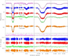 |
Fig. 12. As in Fig. 9, but for ASAS-073, with the ASAS I-band curve added, and shifted vertically for clarity. Without the shift, it would overlap with IMITSuME. The orbit is circular, so the phase of pericentre passage is not defined. |
This agreement suggests that our temperature scale is correct, but it causes problems when we compare with isochrones (Fig. 13). For the given masses and our metallicity of −0.27 dex, one would expect temperatures at the main sequence of around 7800 K for the primary and 5400 K for the secondary. Meanwhile, our values are 1000–1400 K lower. Also the available literature estimates (i.e. Ammons et al. 2006; Gaia Collaboration 2018) give values around 6300 K. The total secondary eclipse and lack of third light allow for direct determination of the observed colours of the primary. From (V − IC) = 0.56(2) mag, (RC − IC) = 0.34(2) mag, (V − RC) = 0.23(2) mag, and calibrations of Worthey & Lee (2011), we get Teff, 1 = 6240(590) K. A similar procedure for the secondary gives 4400(150) K. Even though the uncertainties are large, these values are well below the ones expected at the main sequence, and in agreement with those in Table 3.
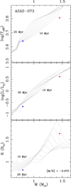 |
Fig. 13. As in Fig. 5, but for the eclipsing binary ASAS-073, and a family of [M/H] = −0.27 isochrones, spanning from log(τ) = 7.0 (10 Myr) to log(τ) = 7.4 (25 Myr), every Δlog(τ) = 0.05 (grey lines). |
Our results can be, at least qualitatively, explained by the young age of the system. The properties of the primary and secondary are best reproduced (within 3σ) by 10- and 25-Myr isochrones, respectively (assuming [M/H] = −0.27 dex). This means the pre-main sequence (PMS) phase. The isochrones in Fig. 13 are shown for ages 10–25 Myr. The age in PARSEC is counted from a position on the Hayashi track, and from a model that is artificially set to have a central temperature of ∼105 K (Bressan et al. 2012). It is uncertain if two protostars of substantially different masses, formed from the same molecular cloud, reached the Hayashi track and this particular temperature at the same moment. If not, a difference in age of ∼15 Myr can be explained. Therefore, we suspect that ASAS-073 may be a rare case of a PMS eclipsing binary. This is not in disagreement with the theory of tidal interactions, which predicts circularisation of the orbit of ASAS-073 after ∼1.5 Myr. We would also like to note that in the UV images from the GALEX satellite, at the position of ASAS-073 there is a strong, point-like source that seems to be surrounded by a fainter extended emission. No X-ray source is related to the target, and no significant emission is seen in cores of Ca H and K lines in the spectra.
The radius and effective temperature of the primary are formally reproduced by “older” isochrones of ages 1.4 and 2.5 Gyr, respectively. Both would require the secondary to be smaller by more than 10%. Discrepancies in radius occur for 0.8 M⊙ stars, but are usually not that significant. Reaching the temperatures predicted at the main-sequence phase and the Gaia distance simultaneously requires a substantial amount of interstellar extinction and reddening, around E(B − V)∼0.2−0.25 mag. Independent comparison with PARSEC isochrones on the mass versus (V − IC) plane clearly shows both components to be ∼0.3–0.4 mag too red for the MS. The E(B − V) given by the Galactic Dust Reddening and Extinction on-line service12 is 0.194(6), which is close to the required value, but would mean that all, or at least the majority, of the dust in the line of sight towards ASAS-073 is located closer than 170 pc, which we find unlikely, considering the target lies in the Galactic disc (b = +5.415°). Also, we measured the equivalent width (EW) of the interstellar sodium D1 line in FEROS and HIDES spectra, and found it to be 0.025(5) Å. According to calibrations by Munari & Zwitter (1997 see also references therein), it should be about 20 times larger to explain E(B − V)∼0.2 mag.
Furthermore, the observed values of l2/l1 are in strong disagreement with those predicted by 1.4 and 2.5 Gyr isochrones, but can be reproduced by the 10–25 Myr isochrones. From the fact that the secondary eclipse is total and well sampled, the flux ratios are robust and very well constrained in all bands, especially in the MITSuME data, and independent on other parameters, like radii or effective temperatures, or the photometric calibrations (see Sect. 4.5). Their inconsistencies with “older” isochrones further support the PMS scenario.
Finally, we checked the Galactic kinematics of ASAS-073. Using the parallax and proper motion from Gaia DR2 and our value of the systemic velocity γ, we calculated the spatial motion components: U = 37.3(3), V = −15.4(3), and W = −18.3(2) km s−1 (no correction for the solar movement has been done). These values put ASAS-073 within the thin disc, at the edge of the space occupied by a moving group called Coma Berenices or “local” (Famaey et al. 2005; Seavroke & Gilmore 2007). Famaey et al. (2005) have shown that ages of stars from this group vary from several to a few hundred million years. This membership, if confirmed, would also support the “young” isochrone age of 10–25 Myr, and make the main sequence stage less probable.
We therefore conclude that ASAS-073 is probably a PMS eclipsing system, and if so, it is valuable for testing models at early stages of stellar evolution. There are not many known PMS DEBs, especially with component masses below 1.5 M⊙. Coronado et al. (2015) listed seven such systems (see references therein) and presented one new candidate. Only two of those binaries are currently in the DEBCat: ASAS J052821+0338.5 (Stempels et al. 2008) and V1174 Ori (Stassun et al. 2004). More recently, four more cases have been reported by Kraus et al. (2015), David et al. (2016 one probably composed of two brown dwarfs), and Lacy et al. (2016). The PMS eclipsing binaries are heavily under-studied, and every new example is highly valuable. The definitive confirmation of the evolutionary state of ASAS-073 requires better knowledge of the temperatures and extinction towards the target. Notably, this system is brighter than the majority of the PMS examples known to date, which makes it a relatively easy target for further studies, which are highly encouraged.
7. Summary
In this study we present physical parameters of three targets from our large program aimed at the characterisation of interesting eclipsing binary systems. In order to quickly but securely measure RVs of secondary components of the presented cases we decided to observe in the IR. This also allowed us to confirm some RV measurements from the optical spectra, and verify that they have not been confused with sidelobes of the CCF or other artefacts. All eclipsing pairs show low mass ratios, which makes fitting an isochrone more difficult than in cases of similar-mass stars. All three examples are, however, very different and interesting in their own way. ASAS-052 is a quadruple-lined (triple in visible light), SB2+SB2 multiple with an eclipsing pair, and all four stellar masses have been estimated. Relative-velocity measurements of the faintest component have only been made in the IR. The astrometric orbit has been determined for the first time, and suggests strong dynamical interactions between pairs Aa+Ab (eclipsing) and Ba+Bb (non-eclipsing). Both ASAS-052 A and ASAS-065 are composed of a solar-analogue primary and a low-mass secondary, but the latter has its parameters measured much more precisely, sufficiently for testing stellar evolution models, and is actually composed of at least three stars, including a distant, low-mass companion. ASAS-065 also allows for precise RV measurements, at the level adequate to search for massive circumbinary planets. Moreover, its significant activity at a relatively old age, not enhanced by rotation, is somewhat unusual. Finally, ASAS-073 is probably a new late-type PMS system, one of the brightest known to date, which provides a great opportunity for further studies.
Our study shows the advantage of IR spectroscopy in observations of low-mass stars. We managed to directly calculate RVs of the faint, cool components with relatively little telescope time. We were able to quickly obtain useful data, crucial for modelling and understanding the nature of the studied systems. There are still many open questions regarding the low-mass stars, and their image will not be complete without proper attention drawn to high-contrast systems. Since the number of well-studied cases is very low, it is still unclear whether or not, for example, the K- and M-type stars paired with F- or G-type primaries show systematic differences with respect to the double-M and double-K binaries. There are potentially many bright DEBs that appear to be single-lined in optical, but may occur to be SB2 in IR. They could be identified as, for example, a by-product of transit search surveys (Beatty et al. 2007; Triaud et al. 2013, 2017). The growing number of high-stability IR spectrographs, like the IRD at Subaru (Kotani et al. 2014) or GIANO at TNG (Origlia et al. 2014), will make it easier to study these stars in more detail, which is something that they truly merit.
It should be noted that not all SB1 systems have unseen secondaries that are cooler and therefore more visible in IR. In a significant number of DEBs, like systems with an evolved giant or some classical Algols, the primary actually has lower Teff, but is significantly larger than the secondary, and contributes more to the overall flux.
IRAF is written and supported by the IRAF programming group at the National Optical Astronomy Observatories (NOAO) in Tucson, AZ. NOAO is operated by the Association of Universities for Research in Astronomy (AURA), Inc. under cooperative agreement with the National Science Foundation. http://iraf.noao.edu/
We define the primary eclipse as the deeper one, and the one during which the primary component (here also hotter) is eclipsed.
Acknowledgments
We would like to thank the anonymous Referee for valuable comments and suggestions, which helped us to improve the work. We would also like to thank the staff of the ESO La Silla, Geneva, and Cerro Tololo observatories, as well as SOAR, TNG, and Subaru telescopes for their support during observations. We also wish to recognise and acknowledge the very significant cultural role and reverence that the summit of Maunakea has always had within the indigenous Hawaiian community. We are most fortunate to have the opportunity to conduct observations from this mountain. This publication is based on data collected: at the Subaru Telescope, which is operated by the National Astronomical Observatory of Japan; through CNTAC proposals CN-2012B-36, CN-2013A-93, CN-2013B-22, CN-2014A-44, and CN-2014B-67; at the European Southern Observatory, Chile under programmes 088.D-0080, 090.D-0061, 091.D-0145; at the Southern Astrophysical Research (SOAR) telescope, which is a joint project of the Ministério da Ciência, Tecnologia, e Inovação (MCTI) da República Federativa do Brasil, the US National Optical Astronomy Observatory (NOAO), the University of North Carolina at Chapel Hill (UNC), and Michigan State University (MSU); with the HARPS-N spectrograph on the 3.58 m Italian Telescopio Nazionale Galileo (TNG) operated on the island of La Palma by the Fundación Galileo Galilei of the INAF (Instituto Nazionale di Astrofisica) at the Spanish Observatorio del Roque de los Muchachos of the Instituto de Astrofisica de Canarias (programme OPT14B 45 from OPTICON common time allocation process for EC supported trans-national access to European telescopes). This research has made use of the Washington Double Star Catalog maintained at the US Naval Observatory. This work has made use of data from the European Space Agency (ESA) mission Gaia (https://www.cosmos.esa.int/gaia), processed by the Gaia Data Processing and Analysis Consortium (DPAC, https://www.cosmos.esa.int/web/gaia/dpac/consortium). Funding for the DPAC has been provided by national institutions, in particular the institutions participating in the Gaia Multilateral Agreement. KGH, EN, and MR acknowledge support provided by the Polish National Science Center through grants no. 2016/21/B/ST9/01613, 2014/13/B/ST9/00902, and 2015/16/S/ST9/00461, respectively. This work was partially supported by JSPS KAKENHI Grant Number 16H01106.
References
- Aitken, R. G. 1903, Lick Obs. Bull., 29, 16 [NASA ADS] [CrossRef] [Google Scholar]
- Alam, S., Ambareti, F. D., Allende Prieto, C., et al. 2015, ApJS, 219, 12 [NASA ADS] [CrossRef] [Google Scholar]
- Ammons, S. M., Robinson, S. E., Strader, J., et al. 2006, ApJ, 638, 1004 [NASA ADS] [CrossRef] [Google Scholar]
- Artigau, É., Kouach, D., Donati, J.-F., et al. 2014, Proc. SPIE, 9147, 914715 [CrossRef] [Google Scholar]
- Asplund, M., Grevesse, N., Sauval, A. J., & Scott, P. 2009, ARA&A, 47, 481 [NASA ADS] [CrossRef] [Google Scholar]
- Bagnuolo, W. G., & Gies, D. R. 1991, ApJ, 376, 266 [NASA ADS] [CrossRef] [Google Scholar]
- Bass, G., Orosz, J. A., Welsh, W. F., et al. 2012, ApJ, 761, 157 [NASA ADS] [CrossRef] [Google Scholar]
- Bate, M. R. 2000, MNRAS, 314, 33 [NASA ADS] [CrossRef] [Google Scholar]
- Beatty, T. G., Fernández, J. M., Latham, D. W., et al. 2007, ApJ, 663, 573 [NASA ADS] [CrossRef] [Google Scholar]
- Bessell, M. S., Castelli, F., & Plez, B. 1998, A&A, 333, 231 [NASA ADS] [Google Scholar]
- Borkovits, T., Albrecht, S., Rappaport, S., et al. 2018, MNRAS, 478, 5135 [NASA ADS] [Google Scholar]
- Boss, A. P. 1993, in The Realm of Interacting Binary Stars, eds. J. Sahade, G. E. McCluskey, & Y. Kondo (Dordrech: Kluwer), 355 [NASA ADS] [CrossRef] [Google Scholar]
- Brahm, R., Jordán, A., & Espinoza, N. 2017, PASP, 129, 034002 [NASA ADS] [CrossRef] [Google Scholar]
- Bressan, A., Marigo, P., Girardi, L., et al. 2012, MNRAS, 427, 127 [NASA ADS] [CrossRef] [Google Scholar]
- Bright, J. C., & Torres, G. 2017, ApJ, 850, 10 [NASA ADS] [CrossRef] [Google Scholar]
- Burdanov, A., Delrez, L., Gillon, M., & Jehin, E. 2017, in SPECULOOS Exoplanet Search and Its Prototype on TRAPPIST, in Handbook of Exoplanets, eds. H. J. Deeg, & J. A. Belmonte (Springer Living Reference Work), 310 [Google Scholar]
- Clausen, J. V., Bruntt, H., Claret, A., et al. 2009, A&A, 502, 253 [NASA ADS] [CrossRef] [EDP Sciences] [Google Scholar]
- Code, A. D., Bless, R. C., Davis, J., & Brown, R. H. 1976, ApJ, 203, 417 [NASA ADS] [CrossRef] [Google Scholar]
- Coelho, P., Barbuy, B., Meléndez, J., et al. 2005, A&A, 443, 735 [NASA ADS] [CrossRef] [EDP Sciences] [Google Scholar]
- Coronado, J., Hełminiak, K. G., Vanzi, L., et al. 2015, MNRAS, 448, 1937 [NASA ADS] [CrossRef] [Google Scholar]
- David, T. J., Hillenbrand, L. A., Cody, A. M., Carpenter, J. M., & Howard, A. W. 2016, ApJ, 816, 21 [NASA ADS] [CrossRef] [Google Scholar]
- Debosscher, J., Aerts, C., Tkachenko, A., et al. 2013, A&A, 556, A56 [NASA ADS] [CrossRef] [EDP Sciences] [Google Scholar]
- Dimitrov, W., Fagas, M., Kamiński, K., et al. 2014, A&A, 564, A26 [NASA ADS] [CrossRef] [EDP Sciences] [Google Scholar]
- Donati, J.-F., Semel, M., Carter, B. D., et al. 1997, MNRAS, 291, 658 [NASA ADS] [CrossRef] [MathSciNet] [Google Scholar]
- Doyle, A. P., Davies, G. R., Smalley, B., Chaplin, W. J., & Elsworth, Y. 2014, MNRAS, 444, 3592 [NASA ADS] [CrossRef] [Google Scholar]
- Fabrycky, D., & Tremaine, S. 2007, ApJ, 669, 1298 [NASA ADS] [CrossRef] [Google Scholar]
- Famaey, B., Jorissen, A., Luri, X., et al. 2005, A&A, 430, 165 [NASA ADS] [CrossRef] [EDP Sciences] [Google Scholar]
- Feiden, G. A., Chaboyer, B., & Dotter, A. 2011, ApJ, 740, 25 [NASA ADS] [CrossRef] [Google Scholar]
- Flower, P. J. 1996, ApJ, 469, 335 [Google Scholar]
- Gaia Collaboration (Prusti, T., et al.) 2016, A&A, 595, A1 [NASA ADS] [CrossRef] [EDP Sciences] [Google Scholar]
- Gaia Collaboration (Brown, A. G. A., et al.) 2018, A&A, 616, A1 [NASA ADS] [CrossRef] [EDP Sciences] [Google Scholar]
- Girard, T. M., van Altena, W. F., Zacharias, N., et al. 2011, AJ, 142, 15 [NASA ADS] [CrossRef] [Google Scholar]
- Girardi, L., Bertelli, G., Bressan, A., et al. 2002, A&A, 391, 195 [NASA ADS] [CrossRef] [EDP Sciences] [Google Scholar]
- Gómez Maqueo Chew, Y., Morales, J. C., Faedi, F., et al. 2014, A&A, 572, A50 [NASA ADS] [CrossRef] [EDP Sciences] [Google Scholar]
- Gray, D. F. 2005, The Observation and Analysis of Stellar Photospheres (Cambridge: Cambridge University Press) [CrossRef] [Google Scholar]
- Hadrava, P. 1995, A&AS, 114, 393 [NASA ADS] [Google Scholar]
- Hayano, Y., Hideki, T., Olivier, G., et al. 2008, Proc. SPIE, 7015, 25 [Google Scholar]
- Hayano, Y., Hideki, T., Shin, O., et al. 2010, Proc. SPIE, 7736, 21 [Google Scholar]
- Hełminiak, K. G., & Konacki, M. 2011, A&A, 526, A29 [NASA ADS] [CrossRef] [EDP Sciences] [Google Scholar]
- Hełminiak, K. G., Konacki, M., Złoczewski, K., et al. 2011, A&A, 527, A14 [NASA ADS] [CrossRef] [EDP Sciences] [Google Scholar]
- Hełminiak, K. G., Konacki, M., Różyczka, M., et al. 2012, MNRAS, 425, 1245 [NASA ADS] [CrossRef] [Google Scholar]
- Hełminiak, K. G., Brahm, R., Ratajczak, M., et al. 2014, A&A, 567, A64 [NASA ADS] [CrossRef] [EDP Sciences] [Google Scholar]
- Hełminiak, K. G., Konacki, M., Ratajczak, M., et al. 2015, ASP Conf. Ser., 496, 76 [NASA ADS] [Google Scholar]
- Hełminiak, K. G., Ukita, N., Kambe, E., et al. 2016, MNRAS, 461, 2896 [NASA ADS] [CrossRef] [Google Scholar]
- Hełminiak, K. G., Ukita, N., Kambe, E., et al. 2017a, A&A, 602, A30 [NASA ADS] [CrossRef] [EDP Sciences] [Google Scholar]
- Hełminiak, K. G., Ukita, N., Kambe, E., et al. 2017b, MNRAS, 468, 1726 [NASA ADS] [CrossRef] [Google Scholar]
- Henden, A. A., Levine, S., Terrell, D., & Welch, D. L. 2015, Abstr., 225, 16 [Google Scholar]
- Iglesias-Marzoa, R., López-Morales, M., Arévalo, M. J., Coughlin, J. L., & Lázaro, C. 2017, A&A, 600, A55 [NASA ADS] [CrossRef] [EDP Sciences] [Google Scholar]
- Irwin, J. M., Quinn, S. N., Berta, Z. K., et al. 2011, ApJ, 742, 123 [NASA ADS] [CrossRef] [Google Scholar]
- Izumiura, H. 1999, Proc. 4th East Asian Meeting on Astronomy (Kunming: Yunnan Observatory), 77 [Google Scholar]
- Jordán, A., Brahm, R., Bakos, G. Á., et al. 2014, AJ, 148, 29 [NASA ADS] [CrossRef] [Google Scholar]
- Jordi, K., Grebel, E. K., & Ammon, K. 2006, A&A, 460, 339 [NASA ADS] [CrossRef] [EDP Sciences] [Google Scholar]
- Kałużny, J., Thompson, I. B., Dotter, A., et al. 2014, Acta Astron., 64, 11 [NASA ADS] [Google Scholar]
- Kambe, E., Yoshida, M., & Izumiura, H. 2013, PASJ, 65, 15 [NASA ADS] [CrossRef] [Google Scholar]
- Kaufer, A., Stahl, O., Tubbesing, S., et al. 1999, The Messenger, 95, 8 [Google Scholar]
- Kervella, P., Thévenin, F., Di Folco, E., & Ségransan, D. 2004, A&A, 426, 297 [NASA ADS] [CrossRef] [EDP Sciences] [Google Scholar]
- Kharchenko, N. V., & Roeser, S. 2009, VizieR Online Data Catalog: I/280 [Google Scholar]
- Klinglesmith, D. A., & Sobieski, S. 1970, AJ, 75, 175 [NASA ADS] [CrossRef] [Google Scholar]
- Kobayashi, N., Tokunaga, A. T., Terada, H., et al. 2000, in IRCS: Infrared Camera and Spectrograph for the SubaruTelescope, eds. M. Iye, & A. F. Moorwood, Proc. SPIE: Optical and IR Telescope Instrumentationand Detectors, 4008, 1056 [Google Scholar]
- Kochanek, C. S., Shappee, B. J., Stanek, K. Z., et al. 2017, PASP, 129, 104502 [NASA ADS] [CrossRef] [Google Scholar]
- Kochukov, O., Makaganiuk, V., & Piskunov, N. 2010, A&A, 524, A5 [NASA ADS] [CrossRef] [EDP Sciences] [Google Scholar]
- Konacki, M., Muterspaugh, M. W., Kulkarni, S. R., & Hełminiak, K. G. 2010, ApJ, 719, 1293 [NASA ADS] [CrossRef] [Google Scholar]
- Koo, J.-R., Lee, J. W., Lee, B.-C., et al. 2014, AJ, 147, 104 [NASA ADS] [CrossRef] [Google Scholar]
- Kotani, T., Kawai, N., Yanagisawa, K., et al. 2005, NCimC, 28, 755 [Google Scholar]
- Kotani, T., Tamura, M., Suto, H., et al. 2014, Proc. SPIE, 9147, 914714 [NASA ADS] [CrossRef] [Google Scholar]
- Kovtyukh, V. V., Soubiran, C., & Belik, S. I. 2004, A&A, 427, 933 [NASA ADS] [CrossRef] [EDP Sciences] [Google Scholar]
- Kozai, Y. 1962, AJ, 67, 591 [Google Scholar]
- Kraus, A. L., Cody, A. M., Covey, K. R., et al. 2015, ApJ, 807, 3 [NASA ADS] [CrossRef] [Google Scholar]
- Kunder, A., Kordopatis, G., Steinmetz, M., et al. 2017, AJ, 153, 75 [NASA ADS] [CrossRef] [Google Scholar]
- Kupka, F., Piskunov, N., Ryabchikova, T. A., Stempels, H. C., & Weiss, W. W. 1999, A&AS, 138, 119 [NASA ADS] [CrossRef] [EDP Sciences] [MathSciNet] [PubMed] [Google Scholar]
- Kurucz, R. L. 1992, in The Stellar Population of Galaxies, eds. B. Barbury, & A. Renzini (Dordrecht: Kluwer Academic Publishers), Proc. IAU Symp., 149, 225 [Google Scholar]
- Kurucz, R. L. 1992, Mem. Soc. Astron. It. Suppl., 8, 14 [Google Scholar]
- Lacy, C. H. 1977, ApJ, 218, 444 [Google Scholar]
- Lacy, C. H. S., Fekel, F. C., Pavlovski, K., Torres, G., & Muterspaugh, M. W. 2016, AJ, 152, 2 [NASA ADS] [CrossRef] [Google Scholar]
- Lastennet, E., & Valls-Gabaud, D. 2002, A&A, 396, 551 [NASA ADS] [CrossRef] [EDP Sciences] [Google Scholar]
- Lee, C.-U., Kim, S.-L., Lee, J. W., et al. 2008, MNRAS, 389, 1630 [NASA ADS] [CrossRef] [Google Scholar]
- Lehmann, H., Borkovits, T., Rappaport, S. A., et al. 2016, ApJ, 819, 33 [NASA ADS] [CrossRef] [Google Scholar]
- Lucy, L. B. 1967, Z. Astrophys., 65, 89 [Google Scholar]
- Mason, B. D., Wycoff, G. L., Hartkopf, W. I., Douglass, G. G., & Worley, C. E. 2001, AJ, 122, 3466 [Google Scholar]
- Marigo, P., Girardi, L., Bressan, A., et al. 2017, ApJ, 835, 77 [NASA ADS] [CrossRef] [Google Scholar]
- Mazeh, T., & Shaham, J. 1997, A&A, 77, 145 [NASA ADS] [Google Scholar]
- Mazeh, T., Prato, L., & Simon, M. 2002, ApJ, 564, 1007 [NASA ADS] [CrossRef] [Google Scholar]
- Mazeh, T., Simon, M., Prato, L., Markus, B., & Zucker, S. 2003, ApJ, 599, 1344 [NASA ADS] [CrossRef] [Google Scholar]
- Mints, A., & Hekker, S. 2017, A&A, 604, A108 [NASA ADS] [CrossRef] [EDP Sciences] [Google Scholar]
- Morales, J. C., Ribas, I., Jordi, C., et al. 2009a, ApJ, 691, 1400 [NASA ADS] [CrossRef] [Google Scholar]
- Morales, J. C., Torres, G., Marschall, L. A., & Brehm, W. 2009b, ApJ, 707, 671 [NASA ADS] [CrossRef] [Google Scholar]
- Munari, U., & Zwitter, T. 1997, A&A, 318, 269 [NASA ADS] [Google Scholar]
- Niemczura, E., Murphy, S. J., SMalley, B., et al. 2015, MNRAS, 450, 2764 [NASA ADS] [CrossRef] [Google Scholar]
- Niemczura, E., Polińska, M., Murphy, S. J., et al. 2017, MNRAS, 470, 2870 [NASA ADS] [CrossRef] [Google Scholar]
- Origlia, L., Oliva, E., Baffa, C., et al. 2014, Proc. SPIE, 9147, 91471E [Google Scholar]
- Piskunov, N. E., Kupka, F., Ryabchikova, T. A., Weiss, W. W., & Jeffery, C. S. 1995, A&AS, 112, 525 [NASA ADS] [Google Scholar]
- Pojmański, G. 2002, Acta Astron., 52, 397 [Google Scholar]
- Pollacco, D. L., Skillen, I., Collier Cameron, A., et al. 2006, PASP, 118, 1407 [NASA ADS] [CrossRef] [Google Scholar]
- Popper, D. M. 1997, AJ, 114, 1195 [NASA ADS] [CrossRef] [Google Scholar]
- Popper, D. M., & Etzel, P. B. 1981, AJ, 86, 102 [NASA ADS] [CrossRef] [Google Scholar]
- Prato, L., Simon, M., Mazeh, T., et al. 2002, ApJ, 569, 863 [NASA ADS] [CrossRef] [Google Scholar]
- Prato, L., Ruíz-Rodríguez, D., & Wasserman, L. H. 2018, ApJ, 852, 38 [NASA ADS] [CrossRef] [Google Scholar]
- Prša, A., & Zwitter, T. 2005, ApJ, 628, 426 [NASA ADS] [CrossRef] [Google Scholar]
- Quirrenbach, A., Amado, P. J., Mandel, H., et al. 2010, Proc. SPIE, 7735, 77351 [Google Scholar]
- Rappaport, S., Vandenburg, A., Borkovits, T., et al. 2017, MNRAS, 467, 2160 [NASA ADS] [Google Scholar]
- Różyczka, M., Kałzny, J., Pietrukowicz, P., et al. 2009, AcA, 59, 385 [NASA ADS] [Google Scholar]
- Rucinski, S. M. 1969, Acta Astron., 19, 24 [Google Scholar]
- Sbordone, L. 2005, Mem. Soc. Astron. It. Suppl., 8, 61 [Google Scholar]
- Schwab, Ch, Jovanovic, N., Feger, T., et al. 2012, Proc. SPIE, 8446, 8446 [Google Scholar]
- Seavroke, G. M., & Gilmore, G. 2007, MNRAS, 380, 1348 [NASA ADS] [CrossRef] [Google Scholar]
- Simon, K. P., & Sturm, E. 1994, A&A, 281, 286 [NASA ADS] [Google Scholar]
- Sitek, M., & Pojmański, G. 2014, AcA, 64, 115 [NASA ADS] [Google Scholar]
- Shappee, B. J., Prieto, J. L., Grupe, D., et al. 2014, ApJ, 788, 48 [NASA ADS] [CrossRef] [Google Scholar]
- Skrutskie, M. F., et al. 2006, AJ, 131, 1163 [NASA ADS] [CrossRef] [Google Scholar]
- Smalley, B. 2004, IAU Symp., 224, 131 [NASA ADS] [CrossRef] [Google Scholar]
- Southworth, J. 2015, ASP Conf. Ser., 496, 164 [NASA ADS] [Google Scholar]
- Southworth, J., Maxted, P. F. L., & Smalley, B. 2004a, MNRAS, 351, 1277 [NASA ADS] [CrossRef] [Google Scholar]
- Southworth, J., Zucker, S., Maxted, P. F. L., & Smalley, B. 2004b, MNRAS, 355, 986 [NASA ADS] [CrossRef] [Google Scholar]
- Stassun, K. G., Mathieu, R. D., Vaz, L. P. R., Stroud, N., & Vrba, F. J. 2004, ApJS, 151, 357 [NASA ADS] [CrossRef] [Google Scholar]
- Stempels, H. C., Hebb, L., Stassun, K. G., et al. 2008, A&A, 481, 747 [NASA ADS] [CrossRef] [EDP Sciences] [Google Scholar]
- Themeßl, N., Hekker, S., Southworth, J., et al. 2018, MNRAS, 478, 4669 [NASA ADS] [CrossRef] [Google Scholar]
- Tkachenko, A., Van Reeth, T., Tsymbal, V., et al. 2013, A&A, 560, A37 [NASA ADS] [CrossRef] [EDP Sciences] [Google Scholar]
- Tokovinin, A., Fischer, D. A., Bonati, M., et al. 2013, PASP, 125, 1336 [NASA ADS] [CrossRef] [Google Scholar]
- Tokovinin, A., Mason, B. D., Hartkopf, W. I., Mendez, R. A., & Horch, E. P. 2015, AJ, 150, 50 [NASA ADS] [CrossRef] [Google Scholar]
- Tokovinin, A., Mason, B. D., Hartkopf, W. I., Mendez, R. A., & Horch, E. P. 2018, AJ, 155, 235 [NASA ADS] [CrossRef] [Google Scholar]
- Torres, G., & Ribas, I. 2002, ApJ, 567, 1140 [NASA ADS] [CrossRef] [Google Scholar]
- Torres, G., Andersen, J., & Giménez, A. 2010, A&ARv, 18, 67 [Google Scholar]
- Torres, G., Sandberg Lacy, C. H., Pavlovski, K., et al. 2014, ApJ, 797, 31 [NASA ADS] [CrossRef] [Google Scholar]
- Torres, G., Sandberg Lacy, C. H., Fekel, F. C., Wolf, M., & Muterspaugh, M. W. 2017, ApJ, 846, 115 [NASA ADS] [CrossRef] [Google Scholar]
- Triaud, A. H. M. J., Hebb, L., Anderson, D. R., et al. 2013, A&A, 549, A18 [NASA ADS] [CrossRef] [EDP Sciences] [Google Scholar]
- Triaud, A. H. M. J., Martin, D. V., Ségransan, D., et al. 2017, A&A, 608, A129 [NASA ADS] [CrossRef] [EDP Sciences] [Google Scholar]
- Valenti, J. A., & Fischer, D. A. 2005, ApJS, 159, 141 [NASA ADS] [CrossRef] [MathSciNet] [Google Scholar]
- Valenti, J. A., & Piskunov, N. 1996, A&AS, 118, 595 [NASA ADS] [CrossRef] [EDP Sciences] [Google Scholar]
- van Hamme, W. 1996, AJ, 106, 2096 [Google Scholar]
- Voges, W., Aschenbach, B., Boller, Th., et al. 1999, A&A, 349, 389 [NASA ADS] [Google Scholar]
- Wheatley, P. J., West, R. G., Goad, M. R., et al. 2018, MNRAS, 475, 4476 [NASA ADS] [CrossRef] [Google Scholar]
- Wilson, R. E., & Devinney, E. J. 1971, ApJ, 166, 605 [NASA ADS] [CrossRef] [Google Scholar]
- Worthey, G., & Lee, H.-C. 2011, ApJS, 193, 1 [NASA ADS] [CrossRef] [EDP Sciences] [Google Scholar]
- Wozniak, P. R., Vestrand, W. T., Akerlof, C. W., et al. 2004, AJ, 127, 2436 [NASA ADS] [CrossRef] [Google Scholar]
- Zahn, J.-P. 1975, A&A, 41, 329 [NASA ADS] [Google Scholar]
- Zahn, J.-P. 1977, A&A, 57, 383 [NASA ADS] [Google Scholar]
- Zucker, S., & Mazeh, T. 1994, ApJ, 420, 806 [NASA ADS] [CrossRef] [EDP Sciences] [MathSciNet] [Google Scholar]
Appendix A: Individual RV measurements
In Tables A.1–A.3 we list all the RVs used in this study. We also give the final measurement errors ϵ and residuals of the fit (O − C), together with the exposure time texp of a given spectrum, and its S/N calculated at around 5500 Å for optical spectra and 12 900 Å for IR. When no measurement is given, lines were either not detected, or blended with another component. The last column shows the telescope/spectrograph used, coded as follows: CC = CTIO 1.5 m/CHIRON, EC = Euler/CORALIE, MF = MPG-2.2 m/FEROS, OH = OAO-188/HIDES, SI = Subaru/IRCS, TH = TNG/HARPS-N.
Individual RV measurements of ASAS-052 A and B used in this work.
Individual RV measurements of ASAS-065 used in this work.
Individual RV measurements of ASAS-073 used in this work.
All Tables
Chemical abundances of ASAS-065 and ASAS-073 and their standard deviations, calculated for elements calculated from more than three spectral parts.
Orbital, photometric, and absolute physical parameters of the three studied eclipsing binaries.
All Figures
|
Fig. 1. Example of the parameter error evaluation with PHOEBE, in the case of ASAS-073. Left panel: evolution of the cost function λ. Peaks represent iterations immediately after the kicks. A more significant (deeper, λ ≃ 1.25) minimum in the parameter hyperspace was found after iteration no. 350. Right panel: mapping the degeneration between Kopal’s modified potentials Ω. The solutions included in the final error calculation are plotted with black dots, and those that were rejected (shallower minimum or still before convergence) are plotted with grey circles. The red × symbol with error bars represents the best fit (lowest λ) and the final 1σ uncertainties. |
| In the text | |
|
Fig. 2. Abundances of ASAS-073 (top panel) and ASAS-065 (bottom panel) from the detailed spectral analysis, compared to solar abundances. Open circles without error bars refer to elements for which fewer than three lines were used, hence errors were not estimated. |
| In the text | |
|
Fig. 3. Model RV curves (blue lines) and measurements (red points) of the eclipsing pair ASAS-052 A. Open symbols and the solid line refer to the primary, and solid symbols and the dashed line to the secondary. The dotted horizontal line marks the systemic velocity of the primary. Residuals (all in km s−1) are shown below. Symbols used for each of the instruments are labelled. The phase zero is set to the pericentre time TP. Phases of primary (P) and secondary (S) eclipses are marked with vertical dotted lines and labelled. |
| In the text | |
|
Fig. 4. Model light curves (white lines) and measurements (coloured points) of ASAS-052. The Y axis shows the observed magnitude, with no vertical shifts. Bands and instruments are labelled. Residuals (O − C) are shown below. For consistency, phase zero is set to the primary eclipse mid-time T0. The phase of pericentre passage is marked with a vertical dotted line and labelled “Per”. Note how the depth of the secondary eclipse changes with wavelength. |
| In the text | |
|
Fig. 5. Comparison of our results for ASAS-052 A with theoretical PARSEC isochrone for the age of 4.0 Gyr and [M/H] = +0.5 dex (solid line) and solar-composition 3.5 Gyr (dashed) on mass vs. temperature (top panel), luminosity (middle panel), and radius (bottom panel) planes. The primary is marked with the red symbol, and the secondary with blue. |
| In the text | |
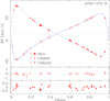 |
Fig. 6. As in Fig. 3, but for the non-eclipsing pair ASAS-052 B. |
| In the text | |
|
Fig. 7. Astrometric orbit of the ASAS-052 B relative to A (large asterisk symbol). The pre-2015 WDS measurements are shown with crosses, and the SOAR data with squares. Dates of some observations are labelled, and the orientation and direction of orbital motion is shown. The inset shows a piece of SOAR interferogram, with the same orientation as the orbit. |
| In the text | |
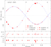 |
Fig. 8. As in Fig. 3, but for the eclipsing binary ASAS-065. |
| In the text | |
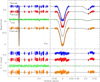 |
Fig. 9. As in Fig. 4, but for ASAS-065, with the MITSuME g′-band curve added. |
| In the text | |
|
Fig. 10. As in Fig. 5, but for the eclipsing binary ASAS-065. The isochrone is for 6.3 Gyr and metallicity of +0.09 dex. |
| In the text | |
|
Fig. 11. As in Fig. 3, but for the eclipsing binary ASAS-073. The orbit of this system is circular, so the zero phase is set to the time of quadrature, and eclipses occur exactly in phases 0.25 and 0.75. |
| In the text | |
|
Fig. 12. As in Fig. 9, but for ASAS-073, with the ASAS I-band curve added, and shifted vertically for clarity. Without the shift, it would overlap with IMITSuME. The orbit is circular, so the phase of pericentre passage is not defined. |
| In the text | |
|
Fig. 13. As in Fig. 5, but for the eclipsing binary ASAS-073, and a family of [M/H] = −0.27 isochrones, spanning from log(τ) = 7.0 (10 Myr) to log(τ) = 7.4 (25 Myr), every Δlog(τ) = 0.05 (grey lines). |
| In the text | |
Current usage metrics show cumulative count of Article Views (full-text article views including HTML views, PDF and ePub downloads, according to the available data) and Abstracts Views on Vision4Press platform.
Data correspond to usage on the plateform after 2015. The current usage metrics is available 48-96 hours after online publication and is updated daily on week days.
Initial download of the metrics may take a while.