| Issue |
A&A
Volume 621, January 2019
|
|
|---|---|---|
| Article Number | A58 | |
| Number of page(s) | 9 | |
| Section | Interstellar and circumstellar matter | |
| DOI | https://doi.org/10.1051/0004-6361/201834274 | |
| Published online | 08 January 2019 | |
Fe I in the β Pictoris circumstellar gas disk
II. Time variations in the circumstellar iron gas
1
Institut d’Astrophysique de Paris, CNRS, UMR-7095, Sorbonne Université,
98bis boulevard Arago,
75014
Paris,
France
e-mail: This email address is being protected from spambots. You need JavaScript enabled to view it.
2
Observatoire de l’Université de Genève,
51 chemin des Maillettes,
1290
Sauverny,
Switzerland
3
Department of Physics, University of Warwick,
Coventry,
CV4 7AL,
UK
Received:
18
September
2018
Accepted:
24
October
2018
Abstract
The young planetary system β Pictoris is surrounded by a debris disk of dust and gas. The gas source of this disk could be exocomets (or “falling and evaporating bodies”, FEBs), which produce refractory elements (Mg, Ca, Fe) through sublimation of dust grains at several tens of stellar radii. Nearly 1700 high resolution spectra of β Pictoris were obtained between 2003 and 2017 using the HARPS spectrograph. In Paper I, we showed that a high signal to noise ratio allows the detection of many weak Fe I lines in more than ten excited levels, and we derived the physical characteristics of the iron gas in the disk. The measured temperature of the gas (~1300 K) suggests that it is produced by evaporation of grains at about 0.3 au (38 R⋆) from the star. Here, we describe the yearly variations of the column densities of all Fe I components (from both ground and excited levels). The drop in the Fe I ground level column density after 2011 coincides with a drop in Fe I excited levels column density, as well as in the Ca II doublet and a ground level Ca I line at the same epoch. All drops are compatible with photoionisation-recombination equilibrium and β Pic like relative abundances, in a medium at 1300 K and at 0.3 au from β Pictoris. Interestingly, this warm medium does not correlate with the numerous exocomets in the circumstellar environnement of this young star.
Key words: stars: individual: β Pictoris / circumstellar matter / comets: general / techniques: spectroscopic
© ESO 2019
1 Introduction
The β Pictoris system is particularly famous for harbouring one of the most massive debris disk in the close neighbourhood of the Sun (Smith & Terrile 1984). Despite being 20 Myr old (Mamajek & Bell 2014), this star has gone through the phase of dissipating dust and gas in its protoplanetary disk, the remnant of which should be a gas-poor dust-poor debris disk. Observations however show that the disk is one of the most dusty gas-poor disks among known debris disk (Artymowicz 1997; Vidal-Madjar et al. 1998) With the age of β Pictoris being much larger than typical timescales of destruction of dust particles (<1 Myr), this led to the conjecture that a replenishment from either collisions or evaporation of hidden planetesimals was necessary to explain the overabundance of dust in this system (Backman & Paresce 1993; Lecavelier et al. 1996).
Moreover, absorption spectroscopy of β Pic revealed the presence of a stable gas component at the star’s radial velocity and variable absorptions attributed to transiting star-grazing exocomets (Ferlet et al. 1987; Beust et al. 1990); see also the review of Vidal-Madjar et al. (1998). The origin of the stable gas disk is still unknown, although highly suspected to be connected to the star-grazing exocomets that strongly evaporate dust and ionized species. Exocomets might be the common vector of gas and dust replenishment in the disk of β Pictoris (Weissman 1984; Lecavelier et al. 1996; Li et al 1998).
The HARPS instrument (see e.g. Pepe et al. 2011) was used to observe β Pictoris for several years, from 2003 to 2017 thanks to large programmes of follow-up (Lagrange et al. 2012, 2018; Kiefer et al. 2014). Thousands of spectra were gathered and several hundreds of exocometary events detected (Kiefer et al. 2014). In Paper I (Vidal-Madjar et al. 2017, VM17 hereafter), stacking the 1686 HARPS spectra collected between 2003 and 2015, we presented the measurements of the physical properties of the iron gas from the detection of a large number of FeI absorption lines, from the ground level up to the 12 969 cm−1 excited level. We conclude that the measured temperature of the gas (~1300 K) coincides with the sublimation temperature of iron from solid compounds, and therefore that this gas is likely produced by the evaporation of grains at about 38 R⋆ or 0.32 au from the star. Moreover, the ground level absorption lines of Fe I presented evidence of two components at different radial velocities. The component centred on the same radial velocity as the one found for the excited levels at 20.41 ± 0.05 km s−1 for which we derived the temperature of 1300 K, and a blueshifted component at 20.07 ± 0.02 km s−1.
Independently, Welsh & Montgomery (2016) found that the ground level Fe I absorption lines in the same β Pic HARPS spectra were experiencing a strong drop of equivalent width between 2011 and 2013. They proposed that the source of the Fe I experiencing the drop is the “D-family” of exocomets identified in Kiefer et al. (2014). These exocomets are composed of strongly evaporating bodies lying about a common orbit, with heliocentric radial velocities in the range +20 to +50 km s−1.
Here we explore in more detail the time variations of both ground and excited levels absorptions of Fe I in the “stable” circumstellar medium, and how they correlate with exocomet activity in the vicinity of the star. The analysis is presented in Sect. 3. The discussions and conclusion are given in Sects. 4 and 5, including a study on the variations also observed in the Ca II doublet (at 3934 and 3968 Å) and the Ca I line (at 4227 Å).
2 Observations
The HARPS spectrograph mounted on the 3.6m telescope of La Silla (ESO Chile) was used to observe β Pictoris from 2003 to 2017 on a (mostly) regular basis (except between 2004 and 2007 and in 2012). Since β Pictoris is only observable in the southern hemisphere summer, the observations were carried out essentially from September to April of each season. The 1D-spectra were extracted via the standard, most recent, HARPS pipeline (DRS 3.5) including localization of the spectral orders on the 2D-images, optimal order extraction, cosmic-ray rejection, wavelength calibration, flat-field corrections, and 1D-reconnection of the spectral orders after correction for the blaze. More details can be found in VM17. We organized the spectra into different samples, each constituting one summer of observation, with the exception of the period 2004–2007. During this period, the average number of spectra observed per summer was 14, which is very small compared to the other periods average (234 spectra per summer). For that reason we created a special sample covering the three summers from 2004 to 2007. This repartition is summarized in Table 1 and Fig. 1.
Because of the high S/N achieved, we were able to detect numerous Fe I absorption lines of the ground level, as well as, of several excited levels. All the detected Fe I lines are listed in Table 2. The energy of the initial electronic levels of the corresponding transitions are summarized in Table 3. In the paper we refer throughout to the individual levels by their energy expressed in cm−1; for example Fe I416 identifies the first excited level at 416 cm−1. We collectively refer to the excited levels as Fe IExc, as opposed to the ground level Fe I0.
The profile of a few individual lines can be found in Paper I, where we also describe the fitting procedure to derive the turbulent parameter, doppler velocity, and column densities.
Repartition of the 2946 HARPS observations.
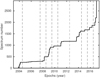 |
Fig. 1 Time distribution of the HARPS observing nights used in our study. The horizontal dotted lines show the limits of the selected observing periods. |
Transition parameters for the detected FeI lines.
Fe I initial levels of the 32 electronic transitions detected in absorption in the HARPS spectrum of β Pictoris.
3 Temporal variations of Fe I circumstellar gas
3.1 Variation of the Fe I ground level
The time variation of the “stable” Fe I ground level absorption lines is given in Table 4, and plotted in Fig. 2. We fitted one single component for each separated period of observation, using the Owens.f code (Hébrard et al. 2002; Lemoine et al. 2002). It fits a Gaussian line-spred-function of 3.6 pixels wide, further broadened by a turbulent parameter b, centered on a radial velocity v and with depth fixed by the column density N and the levels transition parameters as given in Table 2. The continuum is fitted simultaneously using a four-degree polynomial. The two Fe I lines of the ground level are plotted on Fig. 2.
The column density changes significantly, first showing a stable value on the order of 2.5 × 1012 cm−2 lasting about seven years, followed by a 3.5σ drop down to about 1.8 × 1012 cm−2, lasting at least four years. This drop of about 30% in the Fe I total column density was noted from the same HARPS observations by Welsh & Montgomery (2016). It seems that the column density began increasing again. Future observations should confirm this recent evolution.
The turbulent parameter b is stable up to a few hundreds of m s−1 indicating this gas ensemble is thermodynamicaly stable over nearly 12 yr of observation. However, we observe a slow and monotonic reddening of the ground level absorption over years up until 2011, followed by a sudden blueshift simultaneous to the column density drop. Thus, the column density variation must be stronger in the red wing than on the blue wing of the Fe I line.
In the light of the two-component model of VM17, it strongly suggests that only the reddest component at 20.4 km s−1 is experiencing the drop. Moreover, we show in Sect. 3.2 that a column density drop is also observed in the absorption lines of the excited levels that are centered on 20.4 km s−1. We revisit the Fe I ground level absorption lines analysis with a two-component model in Sect. 3.3.
Properties of the FeI gas over the different epochs of observations, evaluated by fitting simultaneously the two absorption lines from the ground state (3859.30 and 3859.70 Å) with a single component.
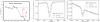 |
Fig. 2 Column density variations in the ground state of the circumstellar Fe I of β Pic. Left panel: temporal variations of the total Fe I0 column density showing a 30 % drop after year 2011. Middle and right panels: sum of the Fe I HARPS fluxes, over the two separate periods, from 2003 to 2011 (solid) and after 2011 (dashed) at the ground state Fe I transition lines wavelengths, 3860 Å (middle panel) and 3824 Å (right panel). |
3.2 Variation of the Fe I excited levels
To further study the time behaviour of the Fe I source, we examine the variations of the Fe I excited levels absorption lines. These evaluations are given in Table 5, as calculated by fitting simultaneously all Fe I excited levels absorption lines with Owens.f. We fixed the radial velocity and turbulent parameters vFe I Exc and bFe I Exc as being common to all excited levels, while the column density can vary separately for each individual level. Only the strongest transitions show well distinguishable absorptions, since the noise wipes the weaker transition signatures away.
For the whole 2003–2015 period VM17 observe that vFe I Exc = 20.41 km s−1, and bFe I Exc = 1.01 ± 0.06 km s−1. From Table 5 we can see that in accordance to VM17, both the v and b of excited levels component remain stable in time about 20.39 and 0.96 km s−1, respectively, except after 2014 where the velocity is more poorly determined. Conversely, the column densities from the excited levels present a time behaviour similar to the ground level with an important drop after 2011.
To more closely investigate the column density variations of the excited levels, we plotted in Fig. 3 all excited levels values (and upper limits), compared to the ground level N variations. The cleanest Fe I416 and Fe I6928 levels and the total column density in all excited levels are highlighted. All levels column densities are normalized to their corresponding median value before the drop, over the 2003–2011 period. To calculate the total column density and their uncertainties, we drew at each epoch 104 series of estimations of the column density at all excited levels according to their measurements distribution, then calculated the sum leading to 104 estimations of the total column density, and determined the final measurement as the median of the sample with errorbars as the 1-σ percentiles.
The drop observed on the total column density of the excited levels is significant at the 6-σ level, with an amplitude of 37 ± 4%. It is larger for the excited levels than for the ground level, for which we measure a 31 ± 2% relative decrease in the column density, leading to a 2-σ significant difference in amplitude. This again suggests that only part of the ground level is undergoing the same drop as the excited levels.
The temporal variations of the Fe I excited levels in vFe I Exc, heliocentric velocity (km s−1), bFe I Exc value (km s−1) and Log N column density (in Log cm−2, identified by the energy level in cm−1) evaluated by fitting simultaneously all excited levels absorption lines, epoch by epoch.
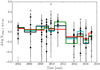 |
Fig. 3 Spread and evolution of the (log) Fe I column density among the 12 excited levels over time. The black circles refer to the column density of each excited level relative to its median value as observed from 2003 to 2017. The grey triangles are upper limits derived from weaker absorptions. A few points outside the plot window are shown with arrows next to the axis. The solid black line shows how the total column density of excited Fe I varies over time. The cyan and green solid lines show the evolution of the column densities derived, respectively, for the Fe I416 and Fe I6928 excited levels. The Fe I0 variations derived in Table 4 are shown as a solid red line. |
3.3 Revisiting the ground level variations with a 2 components model
It has been proposed by VM17 that the absorption lines of the ground level can be divided into 2 components, one of which, at about 20.4 km s−1, is common with excited levels transition lines, and a second one lying at about 20.0 km s−1. In the rest of the paper, we will refer to these 2 hypothesized components as the red component and the blue component, respectively.Besides the variations observed in the excited levels, additional clues suggest two components might be indeed present in the Fe I ground level lines.
First, as observed in Sect. 3.1, the velocity variations of the one-component fit of the Fe I0 absorption lines show that simultaneously to the column density drop there is a blueward shift of the centroid wavelength, suggesting that only the red part of the lines undergoes a drop. Second, the amplitude of the drop in ground level column density is 2-σ lower than the excited levels column density drop suggesting that only a part of the total amount of Fe I in ground level is vanishing. Revisiting the analysis of the Fe I0 absorption lines using a two-component model should confirm these assertions.
From the fit of the excited levels absorption lines in Table 5, the radial velocity of the red component fluctuates about the average value v2 = 20.39 km s−1, without anytrend. We will thus assume that the red component radial velocity is constant and fix it to this value. We then proceed to atwo-component fit of the ground level absorption line, adding a new component and letting all parameters free except v2. The results are given in Table 6.
We findthat the derived radial velocity of the blue component is weakly fluctuating around the average value v1 = 19.77 km s−1. However, the derived turbulence parameters have strong scatters with values lower than 0.05 km s−1 for b1 and as high as 1.5 km s−1 for b2. This is not surprising since we are fitting strongly blended features. Other parameters should be fixed to lower such overfitting effects.
We thus fix both radial velocities v1 and v2 to, respectively, 19.77 and 20.39 km s−1. This time the values of the turbulent parameters are better behaved, with b1 ~ 0.11 ± 0.02 km s−1 and b2 ~ 0.77 ± 0.09 km s−1. The two periods 2015–2016 and 2016–2017 stands aside: as for the excited levels the transition line is not well fit with the common model (for excited levels we measured v ~ 20.20 km s−1). This shift is likely to be imputed to the upgrade of the instrument done in June 20151. Fortunately, it does not impact the measurement of the column density, so the 2015–2017 period remains valuable for the present analysis.
The measured ground-level column density variations in each component are plotted in Fig. 4. The column density of the blue component is found monotonically decreasing, while the red component undergoes a strong drop. This difference is especially pronounced between 2011 and 2013 during the drop, with the red component column density divided by a factor of two, and the blue component remaining essentially stable. Interestingly, the red variations follow well the excited levels variarions with a slight increase of column density between 2003 and 2011.
A Pearson’s R test shows that the total excited levels column density calculated in Table 5 explains the variations of the red component with R = 0.87 (null-hypothesis rejection probability p = 9.8 × 10⁻⁴), while it only explains the variations of the blue component with R = 0.59 (p = 0.074). This means that the red component measurements, having also smaller errorbars (~0.02) than the blue component column density (~0.06), are much better explained by the variations in excited level. However it is difficult to firmly conclude on the compatibility of the blue component column density variations with the excited levels, because although they have larger scatter, they also have larger measurement uncertainties.
Conducting another Pearson’s R test on linear relationship of the components column density with time shows that the blue component is better explained by a continuous decrease through the different epochs, with R = −0.90 (p = 3.7 × 10⁻⁴), while the red component has only R = −0.56 (p = 0.093).
The redand the blue are thus most likely uncorrelated, and the drop in the ground level column density is better explained, as initially suspected, by only the variation of a single component centered on 20.4 km s−1. Observing this red component in the absorption lines of both excited and ground levels, and keeping in mind the measured temperatureof this medium by VM17 (1300 K), leads to infer that the dropping component is located at close distance (~38 R⋆) to the star and varies from a yet unknown process, perhaps exocomets activity drop, as proposed by Welsh & Montgomery (2016) and studied in further detail in Sect. 4.
Since there is no evidence for a blue component in the excited levels lines, it should thus be located at larger distance to the star, certainly several AU where temperatures are much lower than 1000 K. This would explain the absence of a correlation with the inner red component. It is moreover strongly pushed-out in the anti-stellar direction, and slowly dissipating. This component might be part of the distant expanding circumstellar gas identified by Brandeker et al. (2004) and Brandeker (2011).
Table of fitting parameters, modelling the Fe I ground level absorption lines with two components.
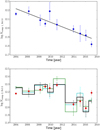 |
Fig. 4 Column density variations measured in the Fe I ground level absorption lines. Top panel: blue component at 19.80 km s−1. The solid black line is a linear model fit of the data. Bottom panel: red component at 20.4 km s−1. The coloured solid lines are the variations observed in excited levels column densities of Fe I416 (cyan), Fe I6928 (green) and total excited Fe I (black), as given in Table 5. They are scaled up to ground level column density. |
4 Exploring the link with β Pictoris circumstellar environnement
4.1 Exocomets activity in the Ca II doublet
It is suggested by Welsh & Montgomery (2016) and VM17 that the circumstellar (CS) Fe I originates from the numerous exocomets observed in the system of β Pictoris. One possible way to test this conjecture would be to determine if variations in the Fe I absorption lines of the circumstellar gas correspond to variations in the cometary activity, or the quantity of particles evaporated from these exocomets.
In the same HARPS spectra as those used here to analyse Fe I lines, there are the Ca II doublet lines that were used in Kiefer et al. (2014) to show that the β Pic’s exocomets separate into two families. The D-family would be composed of strongly evaporating comets about a common orbit, while the S-family would be composed of older comets with smaller amounts of gas released in the circumstellar medium. The D-family absorption signatures are all located within the −10 to 50 km s−1 range in the β Pic rest frame, while the S-family signatures are scattered on a wider velocity range, spanning from −100 to 150 km s−1.
To quantify the cometary activity around β Pictoris, we can calculate the average absorption depth in different velocity domains of the Ca II normalized spectrum. In the small region about the tip of the circumstellar line that reaches almost zero, there could be deep features strongly blended with the circumstellar line; we thus first excluded that region from the analysis, within the range bounded by the instrument resolution (± 2.6 km s−1) about 21.57 km s−1, the tip of the CS line close to the β Pic systemic velocity. We fixed the velocity domain for the D-family to be +5–25 km s−1 and for the S-family to be 50–100 km s−1. These two domains are not overlapping and are centered on the core regions of each family detection statistics, as found in Kiefer et al. (2014).
The reference spectrum that is divided out of the spectra contains the stellar lines and the stable circumstellar and interstellar components. Thus, in the normalized spectra, only flux variations due to exocomet absorption or circumstellar disk fluctuations remain.
The average absorption depth (AAD, hereafter) is measured by averaging each normalized spectrum over the specified spectral band. It is thus proportional to the equivalent width, by a factor Δλ, the wavelength width of the calculation window. Therefore, as long as the absorbing medium is optically thin, this quantity reflects the amount of materials released in the circumstellar medium by transiting exocomets. It also provides information on the typical depth of signatures that are present in the spectrum within the velocity bounds.
Most of the time, several spectra are observed on the same night. This allows us to obtain an average AAD per night, a measure of exocometary activity during a single night. Averaging these night-based AAD over each of the periods considered in this paper (Table 1) we get a measure of how much the exocometary activity varies through time from one period to the other. It could then be compared to the Fe I variations in Fig. 4. Using the night-based AAD for this computation, rather than averaging over all spectra of a given period, makes more sense, because it prevents nights with many collected spectra to dominate the period-based AAD. These average absorption depth are plotted for each exocomet family in Fig. 5.
As can be seen, there are no obvious long-term variations or sudden drops in the exocomet activity. On the contrary, the measurements scatter and the error bars show that the total quantity of particles evaporated from the many transiting exocomets is variable even within a given period. Thus, we see no evidence here for any correlation between exocomet activity and Fe I disk column densities.
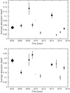 |
Fig. 5 Average absorption depth variations in the co-added Ca II K and H absorption spectra. Top panel: S-familly, between 50 and 100 km s−1. Bottom panel: D-familly, between 5 and 25 km s−1. The marker size is proportionnal to the number of nights where β Pic was observed by HARPS in each period (see Table 1). The errorbars indicate the scatter of average absorption depth during each period. See text for explanations. |
4.2 Variability in the core of the Ca II CS line
We first excluded the strongly blended CS line region (0 ± 5 km s−1), since we were initially interested in exocomet absorption. However, the CS line region incorporates circumstellar disk variations, as well as exocomets transit signatures. It is interesting to see if significant Ca II variations show up in that region, even thoughwe cannot know their origin. We plotted the AAD variation in this domain in Fig. 6.
This time, we observe a neat decrease in average absorption depth. The varying blended features in that region have an average depth of about 0.68 ± 0.03 in 2003–2011 and decrease to 0.50 ± 0.04 in 2013–2017, for a total 3.6σ drop of 26%along the 14 yr of observations. This is comparable to the measured drop of column density of Fe I. This variation is confirmed by measuring a flux increase in the 5 pixels at the tip of the K-line from 0.0096 ± 0.0012 to 0.0196 ± 0.0021 in arbitrary unit, and from 0.0166 ± 0.0019 to 0.037 ± 0.0064 at the tip of the H-line.
Given that the average absorption depth is directly proportional to equivalent width, and thus at first approximation to average column density in the absorbing medium, we see that both Ca II medium and Fe I medium varied in about the same proportions.This has implications on the Fe and Ca relative abundance in the circumstellar medium close to the star, that we explore in more detail in Sect. 5.
In conclusion, the variations experienced by the Fe I components column density are likely connected to Ca II variations in the circumstellar medium. Ca and Fe are thus part of a common reservoir that suddenly dissipated between 2011 and 2013. We cannot firmly identify the origin of these variations, which could be either large low-velocity exocomets or local gas disk inhomogeneities. The exocomets scenario is however less likely as they would have to be disconnected to the already known exocomets which families show no sign of long-term or sudden variations.
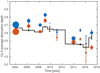 |
Fig. 6 Average absorption depth (AAD) variations in the Ca II circumstellar line region 0 ± 5 km s−1. In blue, the K-line AAD and in red the H-line. They are compared to the total Fe I ground level column density variations in Table 4. The marker size is proportionnal to the number of nights where β Pic was observed by HARPS in each period (see Table 1). For the sake of comparison, the Fe I column densities arescaled to the Ca II AAD median. |
5 Discussing the relation between Ca and Fe
5.1 Implication for the Fe II/Fe I ionization ratio
Independently in both K and H line of the Ca II doublet, we measure an average absorption depth drop of about 0.36 ± 0.04. The average K/H-line ratio of the dropped Ca II component is therefore about 1 ± 0.2. Comparing the individuals AAD of K and H lines in Table 7 leads to a refined K/H ratio closer to 1.2. Thus, the Ca II varying medium is likely not fully saturated. In terms of equivalent width, with the core of the variation concentrated within ± 5 km s−1 of β Pictoris velocity, we can estimate that
 (1)
(1)
The lower limit from simple linear relation between equivalent width and column density in the K and H lines gives that the variation of the column density of Ca II should be ΔNCa II > 4.5 × 1011 cm−2. Using Somerville (1988) equivalent width ratio method, best to use in close-to-saturated cases, we find a range of possible column densities for a ratio of 1.2:
 (2)
(2)
This should be compared to the ΔNFe I = (7.5 ± 0.9) 1011 cm−2 lost during the 2011–2013 drop in the ground level column density. Assuming that Ca is fully ionized below 1 au (Fernández et al. 2006), we can obtain an estimation of the abundance of Ca with respect to Fe in this medium, by calculating ΔNCa II∕ΔNFe I. We find a ratio of about
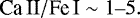 (3)
(3)
Therefore, Ca II and Fe I are almost as abundant in this medium. If it follows β Pic standard abundances (Roberge et al. 2006), with Fe/Ca ~ 15, then we must have Fe II/Fe I ~ 15–75, implying a low ionization rate for Fe. This is in fairly good agreement with the results of VM17, proposing that Fe I/Fe II ≲ 1 in the 20.4 km s−1 component at 1300 K.
Variation of the Ca II average absorption depth and average flux around Ca II K and H circumstellar lines.
5.2 Ca I line variations
In the HARPS spectra, we also found a Ca I circumstellar absorption line about 4226.728 Å, as plotted on Fig. 7. Measuring its variation allow comparing Ca I and Fe I and determining independently the Ca-to-Fe abundance ratio. We thus analysed as for Fe I the variation of the column density in this line using Owens.f. The results are given in Table 8, and compared to Fe I and Ca II variations in Fig. 8.
Again we found a 2-σ significant drop of column density compatible with 30% between 2011 and 2013. The measured column density variation is ΔNCa I = (1.54 ± 0.70) × 108 cm−1. This means that Ca I, Ca II and Fe I variations are all compatible and most likely originate from a common medium.
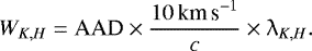
First comparing the column density variation of Ca I, to the one estimated above for Ca II, we find that indeed Ca is almost fully ionized with a ratio Ca II/Ca I ~ 104, much higherthan what primarily found by Hobbs et al. (1985) but closer to the theoretical estimations of Fernández et al. (2006). Second, comparing this Ca I variation to ΔNFe I we find that Fe I is ~5000 (± 2400) times more abundant than Ca I. If originating from a common medium, then according to photoionisation-recombination balance (Lagrange et al. 1995), Ca and Fe should follow, at a given distance to the central star, a one-to-one correspondance in first ionization ratio
 (4)
(4)
Assuming that NFe ~ NFe II and NCa ~ NCa II is a fairly good approximation even if Fe II/Fe I ~ 10. In this case, we derive an abundance ratio Fe/Ca of about 25 (± 12). This is compatible with the solar value for this ratio ~15 (Lodders 2003, 2010) and the value found in β Pic by Roberge et al. (2006), 15 ± 10.
We can also confirm that Fe ionisation ratio is low with the direct measurement of Fe II/Fe I ~ 30–100, using the above formula and the estimation of NCa I∕NCa II.
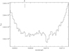 |
Fig. 7 Ca I absorption line at 4226.728 Å with a shift of 20 km s−1. All HARPS spectra from 2003 to 2017 are here co-added. |
Variation of the Ca I velocity shift, b value and column density evaluated by fitting the ground base line at 4226.728 Å.
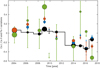 |
Fig. 8 Scaled-to-median Ca I column density variations at 4226.728 Å, in green, compared to Ca II-K (in blue), Ca II-H (in red) and Fe I variations (black). Absolute values for Ca I column densities are reported in Table 8. The median of all datasets was shifted to 0. The size is proportional to the number of observed nights for Ca II, while it is proportional to S/N for Fe I and Ca I, as given in Tables 7, 4, and 8, respectively. |
6 Conclusion
To summarize the reported results, we observed the following in the circumstellar gas disk of β Pictoris that:
The Fe I ground level column density drop of 2011–2013 is also observed in the Fe I excited levels absorption lines centered around velocity 20.4 km s−1.
The blue and red components of Fe I0 absorption lines have different variabilities, with the 20.4 km s−1 being more compatible with a sudden drop, while the blue component seems to have an independent behaviour.
A varying Ca II component is present in the circumstellar line region, whose equivalent width is dropping in average with an amplitude comparable to that of Fe I.
The Ca I circumstellar line also experiences a drop between 2011 and 2013. This drop is compatible with β Pic-like relative abundances for Ca and Fe.
The varying component of Fe has a low ionisation ratio, in agreement with VM17 results.
First, we conclude that the VM17 1300 K medium at 20.4 km s−1 contains not only Fe, but also Ca, and both stand at photoelectric equilibrium. It is located at close distance to the star ~38 R⋆ to sustain the 1300 K temperature and the high ionisation ratio of Ca. The Fe I blue component is likely not connected to this inner disk and belongs to a colder outer location with different photoionization conditions, possibly from recombination of Fe II beyond 100 AU, as described by Brandeker et al. (2004) and Brandeker (2011).
Second, although the Ca II absorptions due to exocomets in the β Pictoris spectrum have a strong variability, they do not show any long term or sudden variations as in the column density of the 20.4 km s−1 component of Fe I. On the other hand, depth variations in the core of the Ca II circumstellar line have a stronger compatibility with the Fe I drop. Large and slow transiting exocomets could be at the origin of such absorptions, blended within the circumstellar line, such as members of the D-family, as suggested by Welsh & Montgomery (2016). However, the absence of correlated variations at larger velocity (up to +30 km s−1 in β Pic rest frame) where most D-family objects lie does not support this hypothesis.
Small-scale disk inhomogeneities with yearly density variations are another alternative scenario. Such variations could be triggered by an outer planet, through direct gravitational interaction or indirectly by changing the flux of incoming dust within an inner disk at 0.3 au. However, in that case a periodic behaviour would be expected. The baseline is not long enough to confirm or exclude periodicity, but a slight increase of the Fe I column density is already observed. The continuation of the monitoring of β Pic optical spectrum with high resolution spectrograph such as HARPS will allow testing this scenario.
Acknowledgements
We thank the anonymous referee for his help on greatly improving the quality of the article. We warmly thank T. Lanz for fruitful discussions on the subject of the present article. F.K. acknowledges support by a CNES fellowship grant. A.L.E, A.V-M and F.K thank the CNES for financial support. This work has been partly carried out thanks to an award from the Fondation Simone et Cino Del Duca. P.A.W. acknowledges support from the European Research Council under the European Unions Horizon 2020 research and innovation programme under grant agreement No. 694513. V. B. and D. E. acknowledgesupport by the Swiss National Science Foundation (SNSF) in the frame of the National Centre for Competence in Research PlanetS, and has received funding from the European Research Council (ERC) under the European Union’s Horizon 2020 research and innovation programme (project Four Aces; grant agreement No 724427). HARPS data were obtained at ESO 3.6m telescope from 2003 to 2017, with Program IDs, 60.A-9036, 072.C-0636, 075.C-0234, 076.C-0073, 076.C-0279, 078.C-0209, 079.C-0170, 080.C-0032, 080.C-0664, 080.C-0712, 081.C-0034, 082.C-0308, 082.C-0412, 084.C-1039, 091.C-0456, 094.C-0946, 098.C-0739, 099.C-0205, 099.C-0599, 184.C-0815, and 192.C-0224
References
- Artymowicz, P. 1997, Ann. Rev. Earth Planet. Sci., 25, 175 [NASA ADS] [CrossRef] [Google Scholar]
- Backman, D. E., & Paresce F. 1993, Protostars and Planets III (Tucson, AZ: University of Arizona Press), 1253 [Google Scholar]
- Beust, H., Vidal-Madjar, A., Ferlet, R., & Lagrange-Henri, A. M. 1990, A&A, 236, 202 [Google Scholar]
- Brandeker, A. 2011, ApJ, 729, 122 [NASA ADS] [CrossRef] [Google Scholar]
- Brandeker, A., Liseau, R., Olofsson, G., & Fridlund, M. 2004, A&A, 413, 681 [NASA ADS] [CrossRef] [EDP Sciences] [Google Scholar]
- Ferlet, R., Vidal-Madjar, A., & Hobbs, L. M. 1987, A&A, 185, 267 [Google Scholar]
- Fernández, R., Brandeker, A., & Wu, Y. 2006, ApJ, 643, 509 [NASA ADS] [CrossRef] [Google Scholar]
- Hébrard, G., Lemoine, M., Vidal-Madjar, A., et al. 2002, ApJS, 140, 103 [NASA ADS] [CrossRef] [Google Scholar]
- Hobbs, L. M., Vidal-Madjar, A., Ferlet, R., Albert, C. E., & Gry, C. 1985, ApJ, 293, L29 [NASA ADS] [CrossRef] [Google Scholar]
- Kiefer, F., Lecavelier des Etangs, A., Boissier, J., et al. 2014, Nature, 514, 462 [NASA ADS] [CrossRef] [EDP Sciences] [Google Scholar]
- Lagrange, A. M., Vidal-Madjar, A., Deleuil, M., et al. 1995, A&A, 296, 499 [NASA ADS] [Google Scholar]
- Lagrange, A. -M., De Bondt, K., Meunier, N., et al. 2012, A&A, 542, A18 [NASA ADS] [CrossRef] [EDP Sciences] [Google Scholar]
- Lagrange, A. -M., Keppler, M., Meunier, N., et al. 2018, A&A, 612, A108 [NASA ADS] [CrossRef] [EDP Sciences] [Google Scholar]
- Lecavelier des Etangs, A., Vidal-Madjar, A. & Ferlet, R. 1996, A&A, 307, 542 [Google Scholar]
- Lemoine, M., Vidal-Madjar, A., Hébrard, G., et al. 2002, ApJS, 140, 67 [NASA ADS] [CrossRef] [Google Scholar]
- Li A., & Greenberg, J. M. 1998, A&A, 331, 291 [Google Scholar]
- Lodders, K. 2003, ApJ, 1220, 591 [Google Scholar]
- Lodders, K. 2010, Astrophys. Space Sci. Proc., 16, 379 [NASA ADS] [CrossRef] [Google Scholar]
- Mamajek, E. E., & Bell C. P. M. 2014, MNRAS, 445, 2169 [NASA ADS] [CrossRef] [Google Scholar]
- Pepe, F., Lovis, C., Ségransan, D., et al. 2011, A&A, 534, A58 [NASA ADS] [CrossRef] [EDP Sciences] [Google Scholar]
- Roberge, A., Feldman, P. D., Weinberger, A. J., Deleuil, M. & Bouret, J.-C. 2006, Nature, 441, 724 [NASA ADS] [CrossRef] [PubMed] [Google Scholar]
- Smith, B. A., & Terrile, R. J. 1984, Science, 226, 1421 [NASA ADS] [CrossRef] [PubMed] [Google Scholar]
- Somerville, W. B. 1988, The Observatory, 108, 44 [NASA ADS] [Google Scholar]
- Vidal-Madjar, A., Lecavelier des Etangs, A., & Ferlet, R. 1998, Planet. Space Sci., 46, 629 [NASA ADS] [CrossRef] [Google Scholar]
- Vidal-Madjar, A., Kiefer, F., Lecavelier des Etangset, A., et al. 2017, A&A, 607, A25 [NASA ADS] [CrossRef] [EDP Sciences] [Google Scholar]
- Weissman, P. R. 1984, Science, 224, 987 [NASA ADS] [CrossRef] [Google Scholar]
- Welsh, B. Y., & Montgomery, S. L., 2016, PASP, 128, 064201 [NASA ADS] [CrossRef] [Google Scholar]
All Tables
Fe I initial levels of the 32 electronic transitions detected in absorption in the HARPS spectrum of β Pictoris.
Properties of the FeI gas over the different epochs of observations, evaluated by fitting simultaneously the two absorption lines from the ground state (3859.30 and 3859.70 Å) with a single component.
The temporal variations of the Fe I excited levels in vFe I Exc, heliocentric velocity (km s−1), bFe I Exc value (km s−1) and Log N column density (in Log cm−2, identified by the energy level in cm−1) evaluated by fitting simultaneously all excited levels absorption lines, epoch by epoch.
Table of fitting parameters, modelling the Fe I ground level absorption lines with two components.
Variation of the Ca II average absorption depth and average flux around Ca II K and H circumstellar lines.
Variation of the Ca I velocity shift, b value and column density evaluated by fitting the ground base line at 4226.728 Å.
All Figures
|
Fig. 1 Time distribution of the HARPS observing nights used in our study. The horizontal dotted lines show the limits of the selected observing periods. |
| In the text | |
|
Fig. 2 Column density variations in the ground state of the circumstellar Fe I of β Pic. Left panel: temporal variations of the total Fe I0 column density showing a 30 % drop after year 2011. Middle and right panels: sum of the Fe I HARPS fluxes, over the two separate periods, from 2003 to 2011 (solid) and after 2011 (dashed) at the ground state Fe I transition lines wavelengths, 3860 Å (middle panel) and 3824 Å (right panel). |
| In the text | |
|
Fig. 3 Spread and evolution of the (log) Fe I column density among the 12 excited levels over time. The black circles refer to the column density of each excited level relative to its median value as observed from 2003 to 2017. The grey triangles are upper limits derived from weaker absorptions. A few points outside the plot window are shown with arrows next to the axis. The solid black line shows how the total column density of excited Fe I varies over time. The cyan and green solid lines show the evolution of the column densities derived, respectively, for the Fe I416 and Fe I6928 excited levels. The Fe I0 variations derived in Table 4 are shown as a solid red line. |
| In the text | |
|
Fig. 4 Column density variations measured in the Fe I ground level absorption lines. Top panel: blue component at 19.80 km s−1. The solid black line is a linear model fit of the data. Bottom panel: red component at 20.4 km s−1. The coloured solid lines are the variations observed in excited levels column densities of Fe I416 (cyan), Fe I6928 (green) and total excited Fe I (black), as given in Table 5. They are scaled up to ground level column density. |
| In the text | |
|
Fig. 5 Average absorption depth variations in the co-added Ca II K and H absorption spectra. Top panel: S-familly, between 50 and 100 km s−1. Bottom panel: D-familly, between 5 and 25 km s−1. The marker size is proportionnal to the number of nights where β Pic was observed by HARPS in each period (see Table 1). The errorbars indicate the scatter of average absorption depth during each period. See text for explanations. |
| In the text | |
|
Fig. 6 Average absorption depth (AAD) variations in the Ca II circumstellar line region 0 ± 5 km s−1. In blue, the K-line AAD and in red the H-line. They are compared to the total Fe I ground level column density variations in Table 4. The marker size is proportionnal to the number of nights where β Pic was observed by HARPS in each period (see Table 1). For the sake of comparison, the Fe I column densities arescaled to the Ca II AAD median. |
| In the text | |
|
Fig. 7 Ca I absorption line at 4226.728 Å with a shift of 20 km s−1. All HARPS spectra from 2003 to 2017 are here co-added. |
| In the text | |
|
Fig. 8 Scaled-to-median Ca I column density variations at 4226.728 Å, in green, compared to Ca II-K (in blue), Ca II-H (in red) and Fe I variations (black). Absolute values for Ca I column densities are reported in Table 8. The median of all datasets was shifted to 0. The size is proportional to the number of observed nights for Ca II, while it is proportional to S/N for Fe I and Ca I, as given in Tables 7, 4, and 8, respectively. |
| In the text | |
Current usage metrics show cumulative count of Article Views (full-text article views including HTML views, PDF and ePub downloads, according to the available data) and Abstracts Views on Vision4Press platform.
Data correspond to usage on the plateform after 2015. The current usage metrics is available 48-96 hours after online publication and is updated daily on week days.
Initial download of the metrics may take a while.