| Issue |
A&A
Volume 697, May 2025
|
|
|---|---|---|
| Article Number | A21 | |
| Number of page(s) | 25 | |
| Section | Planets, planetary systems, and small bodies | |
| DOI | https://doi.org/10.1051/0004-6361/202453568 | |
| Published online | 30 April 2025 | |
Abundances of refractory ions in Beta Pictoris exocomets
1
Institut d’Astrophysique de Paris, CNRS, UMR 7095, Sorbonne Université,
98 bis boulevard Arago,
75014
Paris,
France
2
Department of Physics, University of Warwick,
Coventry
CV4 7AL,
UK
3
LESIA, Observatoire de Paris, Université PSL, CNRS,
5 Place Jules Janssen,
92190
Meudon,
France
★ Corresponding author; vrignaud@iap.fr
Received:
20
December
2024
Accepted:
18
March
2025
β Pictoris is a young A5V star known for harbouring a large number of cometary-like objects (or exocomets) that frequently transit the star and create variable absorption signatures in its spectrum. The physical and chemical properties of these exocomets can be probed by the recently introduced curve of growth approach, which enables column densities measurements in cometary tails using absorption measurements in numerous spectral lines. Through this approach, we present a new study of archival spectra of β Pic obtained with the Hubble Space Telescope, the HARPS spectrograph, and at the Mont John University Observatory aimed at constraining the abundance of refractory ions in β Pic exocomets. We studied 29 individual objects, all of which were observed in Fe II lines (used as a reference ion) and at least one other species (e.g. Ni II, Ca II, Cr II). We find that the refractory composition of β Pic exocomets is stable overall, especially for singly ionised species, and consistent with solar abundances. This outcome validates the use of the curve of growth approach to study exocometary composition. We also show that some ions, such as Ca II, are significantly depleted compared to solar abundances, which allowed us to constrain the typical ionisation state in β Pic exocomets. We find that most refractory elements (e.g. Mg, Ni, Fe) are split into similar fractions between their first and second ionisation states, with the exception of Ca, which is mostly ionised twice. A strong correlation between the Al III/Fe II ratio and radial velocity is also found, showing that the most redshifted exocomets tend to be more ionised. These results open the way for further modelling of exocomets in order to unveil their composition and the physical processes that affect their tails.
Key words: techniques: spectroscopic / comets: general / stars: individual: Beta Pic
© The Authors 2025
 Open Access article, published by EDP Sciences, under the terms of the Creative Commons Attribution License (https://creativecommons.org/licenses/by/4.0), which permits unrestricted use, distribution, and reproduction in any medium, provided the original work is properly cited.
This article is published in open access under the Subscribe to Open model. Subscribe to A&A to support open access publication.
1 Introduction
β Pictoris (β Pic) is a well-studied young (20 Myr; Miret-Roig et al. 2020) planetary system that often serves as a benchmark for studying planetary system formation and evolution. It has attracted significant attention due to its prominent debris disc (Smith & Terrile 1984), which is rich in gas and dust (Vidal-Madjar et al. 1986; Roberge et al. 2006; Apai et al. 2015) and extends over hundreds of au. The system is also known for hosting planets (Lagrange et al. 2010, 2019; Nowak et al. 2020) and a large number of exocomets (Ferlet et al. 1987; Zieba et al. 2019; Lecavelier des Etangs et al. 2022). In fact, β Pic is by far the star showing the most intense exocomet activity, with hundreds of objects detected so far using transit spectroscopy (Kiefer et al. 2014b). Other systems with reported exocomets (typically A-type stars, such as HD 172555 and 49 Cet) generally show much weaker activity (Kiefer et al. 2014a; Montgomery & Welsh 2012; Rebollido et al. 2020; Strøm et al. 2020). Exocomets are of high scientific interest, as they provide valuable insights into the physical and dynamical processes occurring in the early stages of planetary system evolution. For instance, it has been proposed that the presence of exocomets in the inner region of the β Pic system is linked to the gravitational perturbation of planets, which can elongate the orbits of small bodies formed at large stellar distances and bring them to the stellar vicinity (Beust & Morbidelli 1996; Beust et al. 2024). Hints of collisions in the β Pic system have also been reported (Rebollido et al. 2024; Chen et al. 2024), providing an alternative scenario for the origin of the exocomets. However, despite extensive observational campaigns over the past decades, the intrinsic properties of the exocomets – such as their composition and production rat – have remained largely unknown. In particular, no abundance measurements have been conducted so far, thus depriving the community of key information to understand their nature and origin.
A significant advancement in the study of exocomets has come with the work of Vrignaud et al. (2024a), who introduced a new approach for analysing spectroscopic transit data termed the ‘exocomets curve of growth’. This approach is based on the fact that the absorption depth of a transiting comet in a set of lines from a fixed species (e.g. Fe II) is generally a simple function of the line parameters (oscillator strength, excitation energy). The comet’s absorption depths can thus be easily fitted to extract the main physical properties of the comet (covering factor, column density) and infer critical information about the excitation states of ions within the transiting gas.
By applying this approach to a comet observed on December 6, 1997, the most recent study of Vrignaud & Lecavelier des Etangs (2024) has shown that the gas excitation in β Pic exocomets is primarily controlled by the photon flux received from the star rather than by electronic collisions. In this socalled radiative regime, the excitation temperature of the gas is set to the stellar effective temperature (~8000 K), and the excitation state is de-correlated from the local properties of the gas (density, kinetic temperature). This regime is typically associated with a low electronic density (ne ≤ 107 cm−3) and close transit distance (d ≤ 60 R⋆). The study of Vrignaud & Lecavelier des Etangs (2024) also showed that the various ions (e.g. Fe II, Cr II, Ni II) detected in the December 1997 comet are characterised by similar radial velocity profiles and excitation states, hinting that they are well mixed. This shared behaviour among the observed ions is of great use for estimating their abundance ratios in exocomets. For instance, the Ni+/Fe+ and Cr+/Fe+ ratios in the December 6, 1997 comet were estimated to be 8.5 ± 0.8 · 10−2 and 1.04 ± 0.15 · 10−2, respectively, which are rather close to the solar Ni/Fe and Cr/Fe values (Vrignaud & Lecavelier des Etangs 2024).
In this paper, we aim to apply the exocomet curve of growth method to all the exocomets detected so far with the Space Telescope Imaging Spectrograph (STIS) on board the Hubble Space Telescope (HST). By analysing the absorption features observed in an extended list of lines from a dozen chemical species, we aim to place strong constraints on the composition of the cometary tails that routinely transit β Pic. This comprehensive analysis will allow us to investigate the physical mechanisms that affect the composition of these tails (e.g. ionisation) and to further our understanding of the chemical diversity within the β Pic system.
The set of observations used in our analysis is presented in Sect. 2. Sections 3 and 4 then describe our modified curve of growth model aimed at analysing several species in a given exocomet simultaneously and its application to a selection of 29 β Pic exocomets observed with HST. The discussion and conclusion are provided in Sects. 5 and 6.
2 Studied observations
2.1 Raw data
Our study is primarily based on high resolution spectroscopic observations of β Pic obtained with the STIS spectrograph on board the HST. Obtained between 1997 and 2024, these spectra cover wavelength ranges between 1600 and 3000 Å and include a large number of spectral lines from various ionised species (e.g. Fe II, Ni II, Si II, Cr II). These lines, particularly from Fe II, have been shown to be a powerful probe of the physical properties of the transiting comets (Vrignaud et al. 2024a; Vrignaud & Lecavelier des Etangs 2024).
Our dataset is completed with spectroscopic observations of β Pic obtained with other instruments very close in time to the STIS data (typically a few hours apart). These additional observations were collected using the Cosmic Origins Spectrograph (COS), also on board the HST; the High Accuracy Radial Velocity Planet Searcher (HARPS) on the European Southern Observation 3.6 m telescope in La Silla, Chile; and the échelle spectrograph on the McLellan 1-m Telescope at the Mount John University Observatory (MJUO) in New Zealand. The COS spectra cover the far-ultraviolet (FUV) range (~1100–1500 Å), while the HARPS and MJUO spectra probe the visible domain. These complementary datasets provide access to spectral lines that were never observed with STIS, such as the 1250 Å S II triplet (COS) and the 3900 Å Ca II doublet (HARPS, MJUO).
The COS and STIS data were retrieved from the MAST archive, while the HARPS data was obtained from the ESO science portal. The MJUO spectra were obtained from Tobin et al. (2019). Only one night, December 6, 1997, was used in our study. A summary of the studied observations is provided in Table B.1.
2.2 Data reduction
The HARPS and STIS data were reduced in a similar manner as described in Vrignaud et al. (2024a). First, the different spectral orders of each spectrum were weighted together and resampled on a common wavelength table. Then, to correct the flux calibration disparity from one observation to another, each spectrum was renormalised by a cubic spline fitted to stable spectral regions (see Fig. 1 of Vrignaud et al. 2024a). Finally, each set of spectra collected during a short time frame (e.g. the December 6 and 19, 1997 HST visits) was averaged together to boost their signal-to-noise ratio and facilitate their analysis. The COS spectra were simply renormalised by their mean value in the 1350–1380 Å range, which does not show spectral variations due to exocomets. Contrary to STIS and HARPS, no chromatic variation of flux calibration was found for the COS data. The MJUO spectra were not renormalised, as Tobin et al. (2019) already provide flux-calibrated data. Finally, all spectra were shifted to the rest frame of β Pic assuming a heliocentric radial velocity of 20 km/s (Gontcharov 2007).
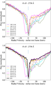 |
Fig. 1 Illustration of the EFS recovery. Top: view of the Fe II 2728 Å line, showing clear spectral variations from one visit to another. Bottom: same line showing the calculated EFS. |
2.3 Exocomet-free spectrum
Once the studied spectra were renormalised to a common flux level, it became easy to visualise the spectral variations caused by the intense cometary activity around the star (see Fig. 1 for Fe II). However, to retrieve the absorption profile of a given exocomet, a reference spectrum of the unocculted star is also required.
This exocomet-free spectrum (EFS) was obtained using a method similar to the one described in Vrignaud et al. (2024a). First, we identified for each spectrum the set of lines affected by comet absorption and the radial velocity ranges at which this absorption occurs (as an example, Table B.1 provides the ranges used for the strongest Fe ir lines). We then averaged for each wavelength pixel all the spectra for which no comet absorption is expected (at that pixel).
This method was used for all lines except the 1850 Å Al III and 3900 Å Ca II doublets. In Al III, the comets studied in the following (which are also detected in Fe II, Ni II, etc.) are often blended with wider, highly variable absorption features that are not observed in singly ionised species. Thus, we did not calculate any EFS for this doublet. Instead, for each exocomet, a continuum was fitted on nearby spectral regions using a cubic spline algorithm and used as a reference spectrum (see Fig. 2). For the HARPS observations of the Ca II doublet, we used the same method as introduced in Kiefer et al. (2014b), which takes advantage of the very high number of available observations of β Pic at these wavelengths (9 000+ HARPS spectra obtained from 2003 to 2024). Finally, for the MJUO data, we used the reference spectrum provided in Tobin et al. (2019).
A sample of spectral lines showing clear comet absorption is provided in Fig. C.1, along with the calculated EFS. For lines where very few observations are available, the recovery of the EFS might be incomplete (e.g. the Fe II 2399 Å line).
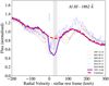 |
Fig. 2 Recovery of a reference spectrum for comet #1 (1997-12-06, grey area) in the Al III 1862 Å line. Unlike other lines, we did not try to recover the EFS. Instead, a continuum is fitted to the observed spectrum (using a cubic spline algorithm), which corrects for the perturbation of broad, shallow exocomets, undetected in other lines. |
2.4 Correlation between cometary features
As pointed out in Vrignaud & Lecavelier des Etangs (2024), the cometary absorptions observed in Fe II lines correlate well with signatures observed in other species (Ni II, Cr II). As an example, Fig. 3 shows two observations of β Pic in Fe II (STIS) and Ca II (HARPS) obtained one hour apart on December 15, 2018. The similarity of the absorption features is striking. In particular, a strong redshifted comet (designated below as comet 18; see table D.1) is clearly visible in both spectra, roughly between 15 and 30 km/s.
The strong correlation between exocometary features observed in lines from different species shows that ions in exocometary tails usually stay mixed thanks to efficient momentum exchange via Coulomb scattering (Vrignaud & Lecavelier des Etangs 2024). This ion mixing is a key feature of β Pic exocomets, as it ensures that the signatures of a comet in a set of lines from different species are not influenced by the spatial distribution of each species individually but rather by the comet geometry as a whole (e.g. covering factor), by the intrinsic spectral properties of each species (e.g. oscillator strengths), and by the global composition of the tail. Combined with the curve of growth approach, this ion mixing greatly facilitates the estimate of abundance ratios in β Pic exocomets.
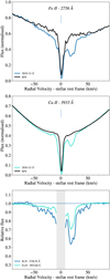 |
Fig. 3 Cometary absorption observed in Fe II (top) and Ca II lines (middle, one hour later) on December 15, 2018. The EFS is plotted with a thick black line. The comparison of the absorption after division by the reference spectrum is given in the bottom panel (the region near the circumstellar line was removed due to a poorer EFS determination in Fe II lines). |
3 A multi-species curve of growth model
3.1 The curve of growth approach
Introduced in Vrignaud et al. (2024a), the curve of growth approach aims at constraining the physical properties of a transiting exocomet observed in spectroscopy. Instead of focusing on a single spectral line, this approach relies on comparing the exocomet absorption depth in many (typically 10–100) lines with diverse oscillator strengths and excitation levels. The dependency of the comet’s absorption depth with the line oscillator strength and excitation energy can provide valuable estimates of the comet’s physical properties (column density, excitation temperature, and size given by the covering factor of the stellar disc).
The study of Vrignaud et al. (2024a) presented a first curve of growth model where a transiting comet is approximated by a cloud with a homogeneous column density covering a limited fraction of the stellar disc and characterised by a uniform excitation temperature. In this model, the average absorption depth ![$\[\overline{\mathrm{abs}}_{l u}\]$](/articles/aa/full_html/2025/05/aa53568-24/aa53568-24-eq1.png) (see definition in Vrignaud et al. 2024a) of the comet in any line of a fixed species (such as Fe II) is given by
(see definition in Vrignaud et al. 2024a) of the comet in any line of a fixed species (such as Fe II) is given by
![$\[\overline{\mathrm{abs}}_{l u}=\bar{\alpha} \cdot\left(1-e^{-\tau_{l u}}\right),\]$](/articles/aa/full_html/2025/05/aa53568-24/aa53568-24-eq2.png) (1)
(1)
with ![$\[\tau_{l u}=\gamma \cdot \frac{\lambda_{l u}}{\lambda_{0}} g_{l} f_{l u} \cdot e^{-E_{l} / k_{B} T}\]$](/articles/aa/full_html/2025/05/aa53568-24/aa53568-24-eq3.png) as the optical depth of the considered line. Here, l and u denote the lower and upper levels of the transition, and λlu, flu, gl, and El indicate its wavelength, oscillator strength, lower level multiplicity, and lower level energy (respectively). The model is characterised by three parameters:
as the optical depth of the considered line. Here, l and u denote the lower and upper levels of the transition, and λlu, flu, gl, and El indicate its wavelength, oscillator strength, lower level multiplicity, and lower level energy (respectively). The model is characterised by three parameters: ![$\[\bar{\alpha}\]$](/articles/aa/full_html/2025/05/aa53568-24/aa53568-24-eq4.png) , the comet’s average covering factor; γ, the typical optical thickness of the studied species (linked to its column density; see Sect. 3.3 below); and T, its excitation temperature. These parameters are, a priori, specific to the radial velocity range where the comet’s average absorption depths are measured and to the considered species (e.g. Fe II). Finally, λ0 is an arbitrary wavelength. As in previous studies, we use λ0 = 2756.551 Å (which is the wavelength of a strong Fe II line) regardless of the studied species.
, the comet’s average covering factor; γ, the typical optical thickness of the studied species (linked to its column density; see Sect. 3.3 below); and T, its excitation temperature. These parameters are, a priori, specific to the radial velocity range where the comet’s average absorption depths are measured and to the considered species (e.g. Fe II). Finally, λ0 is an arbitrary wavelength. As in previous studies, we use λ0 = 2756.551 Å (which is the wavelength of a strong Fe II line) regardless of the studied species.
Despite its simplicity, this one-zone model happens to fit most of the observed variable absorptions in the β Pic spectrum well (see Sect. 4). However, Vrignaud & Lecavelier des Etangs (2024) noted that some cometary signatures can slightly deviate from this model and are thus better described by the transit of several gaseous components with various sizes and optical depths.
Vrignaud & Lecavelier des Etangs (2024) therefore introduced a more sophisticated curve of growth model in which a transiting comet is represented with two gaseous components: a dense core and a surrounding thinner envelope. This new model has five parameters: ![$\[\overline{\alpha_{t}}\]$](/articles/aa/full_html/2025/05/aa53568-24/aa53568-24-eq5.png) , the total comet’s covering factor;
, the total comet’s covering factor; ![$\[\overline{\alpha_{c}}\]$](/articles/aa/full_html/2025/05/aa53568-24/aa53568-24-eq6.png) , the covering factor of the core component; γc, the typical optical thickness in the core component; γe/γc, the optical thickness ratio between the external and core components; and T, the excitation temperature throughout the comet. The average absorption depth
, the covering factor of the core component; γc, the typical optical thickness in the core component; γe/γc, the optical thickness ratio between the external and core components; and T, the excitation temperature throughout the comet. The average absorption depth ![$\[\overline{\mathrm{abs}}_{l u}\]$](/articles/aa/full_html/2025/05/aa53568-24/aa53568-24-eq7.png) of the comet in any line of the studied species is then expressed as
of the comet in any line of the studied species is then expressed as
![$\[\overline{\mathrm{abs}}_{l u}=\bar{\alpha}_{\mathrm{c}} \cdot\left(1-e^{-\tau_{\mathrm{c}, l u}}\right)+\bar{\alpha}_{\mathrm{e}} \cdot\left(1-e^{-\tau_{\mathrm{e}, l u}}\right),\]$](/articles/aa/full_html/2025/05/aa53568-24/aa53568-24-eq8.png) (2)
(2)
![$\[\begin{aligned}& \tau_{\mathrm{c}, l u}=\gamma_{\mathrm{c}} \cdot \frac{\lambda_{l u}}{\lambda_0} g_l f_{l u} e^{-E_l / k_B T}, \\& \tau_{\mathrm{e}, l u}=\gamma_{\mathrm{e}} \cdot \frac{\lambda_{l u}}{\lambda_0} g_l f_{l u} e^{-E_l / k_B T},\end{aligned}\]$](/articles/aa/full_html/2025/05/aa53568-24/aa53568-24-eq9.png)
and where ![$\[\bar{\alpha}_{\mathrm{e}}\]$](/articles/aa/full_html/2025/05/aa53568-24/aa53568-24-eq10.png) and γe, respectively the covering factor and typical optical thickness of the outer envelope, are given by
and γe, respectively the covering factor and typical optical thickness of the outer envelope, are given by
![$\[\begin{aligned}& \bar{\alpha}_{\mathrm{e}}=\bar{\alpha}_{\mathrm{t}}-\bar{\alpha}_{\mathrm{c}}, \\& \gamma_{\mathrm{e}}=\gamma_{\mathrm{c}} \cdot \frac{\gamma_{\mathrm{e}}}{\gamma_{\mathrm{c}}}.\end{aligned}\]$](/articles/aa/full_html/2025/05/aa53568-24/aa53568-24-eq11.png)
Again, the five model parameters are – a priori – specific to the studied species (Fe II, Ni II, etc.) and to the radial velocity range where the comet’s average absorption depth is measured.
3.2 Fitting several species simultaneously
In previous studies, these models were mostly applied to Fe II lines, which are very numerous and show strong comet absorption. However, Vrignaud et al. (2024a) showed that the absorption signatures of individual exocomets in lines from different species (Ni II, Cr II) tend to have the same shape and to follow the same curve of growth as Fe II. In other words, the comet geometry (e.g. ![$\[\bar{\alpha}, \bar{\alpha}_{c}\]$](/articles/aa/full_html/2025/05/aa53568-24/aa53568-24-eq12.png) ) and excitation temperature (T) constrained by Fe II lines also apply to other species.
) and excitation temperature (T) constrained by Fe II lines also apply to other species.
In the following, we thus assume that exocometary gaseous tails always remain well mixed regardless of their overall shape. This hypothesis allows us to introduce a multi-species curve of growth model able to fit several species simultaneously. Going back to Eqs. (1) and (2), we assume that the geometric parameters (![$\[\bar{\alpha}\]$](/articles/aa/full_html/2025/05/aa53568-24/aa53568-24-eq13.png) for Eq. (1) and
for Eq. (1) and ![$\[\bar{\alpha}_{t}, \bar{\alpha}_{c}\]$](/articles/aa/full_html/2025/05/aa53568-24/aa53568-24-eq14.png) , and γe/γc for Eq. (2)) and the excitation temperature (T) are the same for all species; only the γ (Eq. (1)) and γc (Eq. (2)) parameters remain specific to each atom or ion. These assumptions allow us to refine Eqs. (1) and (2) into Eqs. (3) and (4):
, and γe/γc for Eq. (2)) and the excitation temperature (T) are the same for all species; only the γ (Eq. (1)) and γc (Eq. (2)) parameters remain specific to each atom or ion. These assumptions allow us to refine Eqs. (1) and (2) into Eqs. (3) and (4):
![$\[\overline{\mathrm{abs}}_{l u, ~i}=\bar{\alpha} \cdot\left(1-e^{-\tau_{l u, ~i}}\right),\]$](/articles/aa/full_html/2025/05/aa53568-24/aa53568-24-eq15.png) (3)
(3)
![$\[\tau_{l u, i}=\gamma_i \cdot \frac{\lambda_{l u}}{\lambda_0} g_l f_{l u} \cdot e^{-E_l / k_B T},\]$](/articles/aa/full_html/2025/05/aa53568-24/aa53568-24-eq16.png)
![$\[\overline{\mathrm{abs}}_{l u, ~i}=\bar{\alpha}_{\mathrm{c}} \cdot\left(1-e^{-\tau_{\mathrm{c}, ~l u, ~i}}\right)+\bar{\alpha}_{\mathrm{e}} \cdot\left(1-e^{-\tau_{\mathrm{e}, ~l u, ~i}}\right),\]$](/articles/aa/full_html/2025/05/aa53568-24/aa53568-24-eq17.png)
![$\[\begin{aligned}& \tau_{\mathrm{c}, l ~u, ~i}=\gamma_{\mathrm{c}, ~i} \cdot \frac{\lambda_{l u}}{\lambda_0} g_l f_{l u} e^{-E_l / k_B T}, \\& \tau_{\mathrm{e}, l ~u, ~i}=\gamma_{\mathrm{c}, ~i} \cdot \frac{\gamma_{\mathrm{e}}}{\gamma_{\mathrm{c}}} \cdot \frac{\lambda_{l u}}{\lambda_0} g_l f_{l u} e^{-E_l / k_B T}.\end{aligned}\]$](/articles/aa/full_html/2025/05/aa53568-24/aa53568-24-eq18.png)
In the above equations, we use the letter i to specify the species associated with the line (l, u). The two models respectively have n + 2 and n + 4 parameters, with n as the number of fitted species.
Studied chemical species sorted by ionisation energy.
3.3 Estimating abundance ratios
Equations (3) and (4) can be fitted to the absorption depths of a given comet in a set of lines from several species in order to constrain the comet geometry, excitation temperature, and typical optical thicknesses of each species (γi for Eq. (3) and γc, i for Eq. (4)). Once constrained, these parameters allow for the estimate of the total column density of each species through (see Vrignaud et al. 2024a; Vrignaud & Lecavelier des Etangs 2024)
![$\[\mathrm{N}_{\mathrm{tot}, ~i}=\frac{4 \varepsilon_0 m_e c}{e^2 \lambda_0} \Delta v ~Z_i(T) ~\gamma_i \bar{\alpha}\]$](/articles/aa/full_html/2025/05/aa53568-24/aa53568-24-eq19.png)
for the one-zone model (Eq. (3)) and
![$\[\mathrm{N}_{\mathrm{tot}, ~i}=\frac{4 \varepsilon_0 m_e c}{e^2 \lambda_0} \Delta v ~Z_i(T) ~\gamma_{\mathrm{c}, i}\left(\bar{\alpha}_{\mathrm{c}}+\left(\gamma_{\mathrm{e}} / \gamma_{\mathrm{c}}\right) \bar{\alpha}_{\mathrm{e}}\right)\]$](/articles/aa/full_html/2025/05/aa53568-24/aa53568-24-eq20.png)
for the two-component model (Eq. (4)). Here, Δv is the radial velocity width of the comet, Zi(T) is the partition function of the considered species, and ϵ0, me, and c are respectively the vacuum permittivity, electron mass, and light velocity. Using the assumption that the geometric parameters are identical for all the studied species, the abundance ratio of two species i, j is then written as
![$\[\left[\frac{i}{j}\right]=\frac{\mathrm{N}_{\mathrm{tot}, ~i}}{\mathrm{~N}_{\mathrm{tot}, ~j}}=\frac{Z_i(T) ~\gamma_i}{Z_j(T) ~\gamma_j},\]$](/articles/aa/full_html/2025/05/aa53568-24/aa53568-24-eq21.png) (5)
(5)
where the γi and γj parameters are replaced by γc, i and γc, j in the case of a two-component model.
4 Application to a sample of comets
4.1 The sample of exocomets
Our study is aimed at measuring the abundance ratio of several atoms and ions (e.g. S I, Fe II, Ni II) in β Pic exocomets by using the available spectroscopic data. To carry out this analysis, we selected a set of 29 comets that appear to be well suited for abundance measurement. All of these comets produce significant, well-individualised absorption in a large number of Fe II lines (used as a reference species) as well as in, at least, one other refractory species (e.g. Cr II, Ni II, Ca II). Basic information on the 29 selected comets is provided in Table D.1. A unique identifier was attributed to each object (e.g. “β Pic C19971206 a” for comet 1) according to the upcoming nomenclature of Lecavelier des Etangs et al. (in prep.). A snapshot of each comet in one strong Fe II line is also provided in Appendix G (online).
4.2 Studied species and line selection
Throughout our cometary sample, we were able to probe a total of 12 refractory species, listed in Table 1, reflecting most of the abundant exocometary species with optically allowed spectral lines in the UV/visible. Most of the studied species are ions, except for S I, which stands out by its fairly high ionisation potential compared to most neutral species (10.36 eV). Other atoms (Fe I, Mg I, Si I, Ca I, etc.) with lower ionisation potentials (≤8 eV) were not detected in any exocomet and are thus not included in the study. This non-detection is probably the result of efficient photo-ionisation. Despite noticeable spectral variations, Al II, Si III, and Si IV were also not included in the study due to a very poor S/N in the 1670 Al II and 1206 Å Si III lines and to highly blended absorption in the 1400 Å Si IV doublet.
For each individual exocomet, it was never possible to probe the abundance of all 12 species simultaneously, either because the appropriate lines were not observed or because the lines were too faint or too saturated to be exploited. As an example, the Cr II/Fe II ratio could be constrained only for the strongest comets (typically when Ntot, Fe II/Δv > 1013 cm−2/km s−1), as cometary signatures in Cr II are usually very faint (a few percent at most). On the other hand, the Mg II/Fe II ratio was estimated only for the faintest comets (Ntot, Fe II/Δv ~ 1012 cm−2/km s−1), as Mg II signatures are easily saturated.
The set of lines used to fit each exocomet was selected carefully. In particular, we did not include lines blended in close multiplets (i.e. when the line separation is lower than the typical width of cometary signatures; see for instance Fig. 4). In addition, lines for which the S/N on the cometary absorption depth is below unity were not included in the fit and neither were those showing spurious features. Finally, we removed the lines for which no reliable EFS can be determined, generally due to an insufficient number of observations. The complete list of lines used throughout the study is given in Table F.1. Most of the line parameters (e.g. λlu, Aul) were obtained from the NIST database (Kramida et al. 2023). Table D.1 also provides the list of line series considered in the fit for each comet.
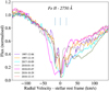 |
Fig. 4 Zoomed-in view of the 2750.13 Å Fe II line (indicated with a solid blue marker). Even if cometary signatures are detected, they are blended with absorptions from other close Fe II lines at 2749.99 and 2750.30 Å (dotted markers). Due to this blending, the triplet was not included in our curve of growth analysis. |
4.3 Fit procedure
Each comet was fitted using a similar procedure. We first measured the average absorption depth (relative to the EFS) of each comet in each line of its selected set. As in Vrignaud et al. (2024a), uncertainties on absorption measurements were estimated by taking into account photon noise (generally between 0.5 and 3%) and systematic errors due to imperfect flux calibration (0.5–1%, estimated by comparing our spectra on stable spectral domains). For each comet, the RV range used to measure its absorption depth was chosen as the range where the absorption is the deepest in order to limit the impact of systematic uncertainties. The RV ranges used in the fits are provided in Table D.1. Next, we fitted the measured absorption depths of each comet using one of the multi-species curve of growth models (Eqs. (3) or (4)) and a Markov chain Monte Carlo algorithm from the emcee python library (Foreman-Mackey et al. 2013). These fits provided constrains on the geometry and excitation temperature of each comet as well as on the γ values of each fitted species. Finally, we estimated the abundance of each fitted species using Eq. (5). To properly estimate uncertainties, this ratio was calculated at each step of the Markov chains.
Comets 22–29 (HST program #17421) were all observed during a rather long time (three to four HST orbits), enough to observe variation in their absorption profile. Each of these comets was analysed once using the HST orbit showing the more individualised and deep absorption (e.g. for comet #22, the second orbit of the April 17, 2024 visit). The specific HST orbits used for these comets are provided in Table D.1.
The one-zone curve of growth model was used for most comets, as it generally provides satisfactory fits. The only exceptions are comets #1, #2, and #6, which appeared to be significantly better fitted with a two-component model (based on the comparison of the Bayesian information criteria (BIC) of the two models).
For comets observed in a set of Fe II lines covering a wide energy range (E/kb typically in the range 0–12000 K), the excitation temperature was set as a free parameter. For other comets, we used a Gaussian prior (T = 9000 ± 500 K) based on values found for exocomets where the excitation temperature could be directly measured. This prior enabled us to estimate column densities in all exocomets, even those for which no direct estimate of the excitation temperature could be performed.
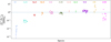 |
Fig. 5 Overview of all abundance measurements performed throughout the 29 exocomet sample, grouped by chemical species. For each species (e.g. S I), the measured ratios with Fe II were divided by the solar ratio of the corresponding elements (e.g. S/Fe), as given by Asplund et al. (2009). The ordering of the species reflect their ionisation energy. Each group of measurements is ordered according to the comet indexes (Table D.1). |
4.4 Results
The curves of growth of the fitted comets can be found in Appendix G. The physical properties of the comets (covering factor, total Fe II column density, excitation temperature) and their measured compositions (abundance ratios) are provided in Tables E.1 and E.2, respectively. All abundance ratios are expressed relative to Fe II, which serves as a reference species. A visual recapitulation of all abundance measurements is also provided in Fig. 5, thus allowing the dispersion of each species to be seen.
5 Discussion
5.1 Excitation temperatures
Before digging into the composition of our cometary sample, it is interesting to look at the excitation temperatures measured in comets #1 to #6 and #8 (Table E.1). In all of these cases, the excitation temperature of the transiting comets remains close to 9000 K. This result validates the conclusion of Vrignaud & Lecavelier des Etangs (2024), which studied in detail the excitation state of Fe II in comet #1. The density in the gaseous cloud surrounding the exocomets is generally sufficiently low for the gas excitation to be controlled by the stellar flux rather than by electronic collisions (radiative regime). In this context, the excitation temperature of the gas is roughly set to the stellar effective temperature (~8052 K; Gray et al. 2006). The slight discrepancy observed between the typical excitation temperature found in exocomets (~9000 K) and the stellar effective temperature could be explained by the presence of absorption lines in the stellar spectrum (as proposed for solar system comets; Manfroid et al. 2021) or by the self-opacity of the transiting gas, which distorts the stellar spectrum received in the innermost regions of the transiting comets.
This consistency of excitation temperature led us to assume that all β Pic exocomets follow a radiative regime, even those for which the gas excitation cannot be directly probed because of an insufficient wavelength coverage. For these comets, we thus applied a Gaussian prior on T of 9000 ± 500 K based on the values found for comets 1-6 and 8 (particularly comets 1, 4, 5, and 8, for which the most accurate values of T could be obtained).
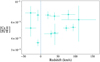 |
Fig. 6 All Ca II/Fe II ratios measured in our exocometary sample as a function of the comet redshift. Horizontal error bars reflect the radial velocity extent of the cometary signatures. |
5.2 Ion abundance
The abundances of most of the singly ionised species (Ca II, Ni II, Si II, Cr II, Mn II, Mg II) relative to Fe II appear to be fairly consistent throughout our cometary sample, with values typically spanning over a factor of two to three at most. As an example, the measured Ca II/Fe II ratio spans from 3 × 10⁻³ to 8 × 10⁻³ (mean: 5.8 × 10⁻³), the Ni II/Fe II ratio spans from 5 × 10⁻² to 10 × 10−2 (mean: 7.6 × 10⁻²), and the Si II/Fe II ratio spans from 0.7 to 1.5 (mean: 0.95). For Ca II, the spread of abundance measurements is wider than the typical uncertainty on each measurement, indicating that the Ca II/Fe II ratio can vary slightly from one comet to another, up to a factor of about three. The origin of this diversity is, however, unclear. No correlation of the Ca II/Fe II ratio with radial velocity is observed (Fig. 6), which could have been expected given that low-velocity and high-velocity comets usually belong to two separated families with different transit distances (Kiefer et al. 2014b). For Ni II, Si II, Cr II, Mn II, and Mg II, the observed abundance distributions are consistent with the estimated error bars. It is therefore difficult to conclude on any diversity in the composition of our comet sample. In addition, the abundance of these species does not seem to be correlated with radial velocity.
A few species, however, exhibit a much wider abundance distribution (Fig. 5). The most obvious one is Al III, with a Al III/Fe II ratio spanning a factor of 20 and ranging from ~0.01 (comets #5, #21) to 0.2 (comet #6). The Al III abundance has been found to be strongly correlated with redshift. The most redshifted comets are usually those that exhibit the strongest Al III absorptions (Fig. 7). The S I abundance in β Pic exocomets also seems fairly diverse, as this atom is clearly detected in comets #5 and #21 (S I/Fe II ~ 9 · 10−3; see Table E.2) but barely noticed in comets #1 and #20 (abundance measurements for other comets were not included in the study due to much larger uncertainties). Here, it is interesting to note that the only two comets found to harbour a significant amount of S I are those that display the weakest Al III signatures (Fig. 7). Contrary to Al III, the S I abundance in β Pic exocomets thus seems to be anticorrelated with redshift, with low-velocity comets showing a higher S I/Fe II ratio. These correlations (or anti-correlations) are very likely linked to the transit distance of the comets since highly redshifted comets are generally closer to the star, meaning that they receive a greater amount of irradiation. According to the model proposed in Beust & Tagger (1993), this would lead to a higher ionisation degree in cometary gas due to a denser and hotter bow shock at the front of the coma. On the contrary, some low-redshift comets appear to be sufficiently far away from the star to allow S I to survive ionisation (and prevent the formation of large amounts of Al III), indicating that the compression mechanisms in their comae are much softer.
Finally, important variations were found for the S II/Fe II ratio (estimated in five exocomets; see Fig. 5), with values ranging from 0.5 to 3. However, these measurements should be taken with caution because Fe II and S II were observed with two different HST instruments (STIS and COS), at different resolutions, and during separate HST orbits, necessarily separated by 96 minutes. Further observations may thus be needed to confirm this diversity in S II/Fe II ratios. For Co II and Zn II, only comet #1 (1997-12-06) could provide constraints on their abundances, with rather large uncertainties. It is therefore impossible to characterise the diversity of exocomet composition regarding these two species.
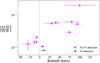 |
Fig. 7 All Al III/Fe II ratios measured in our cometary sample as a function of the comet redshift. Horizontal error bars reflect the radial velocity extent of the cometary signatures. The two violet markers indicate the two comets with clear S I detections (see text). |
5.3 Link between abundances and ionisation energies
Figure 5 shows that the typical abundances of the studied species in β Pic exocomets are generally consistent with solar abundances. For instance, the exocometary Si II/Fe II ratio is close to the solar Si/Fe ratio, ≃1. These quasi-solar values hint that the first ionisation degree is probably a major form of the studied elements. However, we also note some discrepancies: S I, Ca II, and Mg II always appear to be depleted (by factors of ~100, 10, and 2, respectively), while Ni II and S II seem to be overabundant (by a factor 1.5 for Ni IIand by 2 to 6 for S II).
To understand this trend, it is useful to plot the average abundances (normalised to the solar values) as a function of their ionisation potentials (Fig. 8; see the numerical values in Table 2). A clear correlation is visible: the more difficult to ionise a species is, the more abundant it is in β Pic exocomets. The observed deviations from solar ratios are thus probably due to a diversity of ionisation states among the studied species. For instance, the depletion of Ca II is probably due to the higher ionisation degree of Ca than other species, as Ca II is much more easily ionised into Ca III (11.87 eV, Table 1) than Fe II into Fe III or Ni II into Ni III (we note that for all of these species, the neutral fraction is expected to be negligible due to photo-ionisation). Similarly, the high ratio of S II/Fe II compared to the solar S/Fe ratio is likely caused by the very difficult ionisation of S II into S III (23.34 eV), which leads a higher fraction of sulphur to remain as S+ in the cometary tails.
In between, the nearly solar ratios found for Mn II, Si II, and Cr II relative to Fe II are consistent with these four species having similar ionisation energies (~16 eV). These solar ratios suggest that the dust sublimation is efficient enough for the composition of the gaseous tail to reflect the dust composition itself, which is probably solar for refractory elements. This result is very different from Solar System comets, for which the composition of the gas is primarily influenced by the varying sublimation rates of the cometary materials. For instance, in some Solar System comets, the Ni/Fe ratio has been found to be strongly super-solar (Manfroid et al. 2021), possibly due to faster sublimation rates for nickel carbonyls – e.g. Ni(CO)4 – compared to iron carbonyls – e.g. Fe(CO)5.
The Al III/Fe II ratio is slightly more difficult to interpret since Al III is ionised twice. A significant fraction of Al is probably retained as Al II, while for neutral or singly ionised species (S I, Ca II, etc.), the fraction in lower ionisation states is either null or negligible. This explains why the Al III/Fe II ratio is generally sub-solar, even if Al III is very difficult to ionise (28.4 eV).
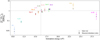 |
Fig. 8 Typical abundances of 11 atoms and ions in β Pic exocomets relative to Fe II and normalised by solar abundances. The numerical values used to build this figure are provided in Table 2. Grey crosses indicate the best-fit model with Saha’s equation (see Sect. 5.4.2). |
Average abundances of 11 refractory species in β Pic exocomets compared to solar ratios.
5.4 The ionisation state
5.4.1 Using the Al III/Fe II ratio
The Al III/Fe II ratio can be used as a probe of the ionisation state in exocometary tails. Here, we consider a given chemical element X (e.g. Fe, Ca) in an exocomet. Assuming that the [X/Fe] and [Al/Fe] ratios are solar, the [X II/X] ratio in the exocomet can be written as (see Appendix A)
![$\[\left[\frac{\mathrm{X}{\small~{\text{II}}}}{\mathrm{X}}\right]_{\mathrm{e}}=\left(\frac{\eta_{\mathrm{Al}}}{\eta_{\mathrm{X}}}+\frac{1}{\eta_{\mathrm{X}} s_{\mathrm{Al}}}\left[\frac{\mathrm{Al} \small~{\text{III}}}{\mathrm{Fe} \small~{\text{II}}}\right]_{\mathrm{e}}\right)^{-1},\]$](/articles/aa/full_html/2025/05/aa53568-24/aa53568-24-eq23.png) (6)
(6)
![$\[\begin{aligned}& s_{\mathrm{Al}}=[\mathrm{Al} / \mathrm{Fe}]_{\odot}, \\& \eta_{\mathrm{X}}=\frac{[\mathrm{X} \small~{\text{II}} / \mathrm{Fe} \small~{\text{II}}]_{\mathrm{e}}}{[\mathrm{X} / \mathrm{Fe}]_{\odot}}, \qquad\quad \eta_{\mathrm{Al}}=\frac{[\mathrm{Al} \small~{\text{II}} / \mathrm{Fe} \small~{\text{II}}]_{\mathrm{e}}}{[\mathrm{Al} / \mathrm{Fe}]_{\odot}},\end{aligned}\]$](/articles/aa/full_html/2025/05/aa53568-24/aa53568-24-eq24.png)
where the index e denotes ratios in the considered exocomet and ηX is the abundance of the singly ionised state of the species X relative to Fe II in solar units.
Our study has shown that the abundances of singly ionised species (Ca II, Cr II, Ni II) relative to Fe II in β Pic exocomets are fairly stable. We can thus make the assumption that ηX and ηAl are fixed parameters independent of the considered exocomet. The value of ηX can be estimated from our measurements (e.g. ηCa = 0.082 ± 0.019, ηFe = 1, ηNi = 1.46 ± 0.20; Table 2). However, the Al II/Fe II ratios of the studied exocomets could not be measured due to the very low stellar flux in the Al II 1670 Å line. This prevented us from directly estimating ηAl. To mitigate this problem, we used the fact that the η value of a given element is primarily controlled by its ionisation potential (Fig. 8). Since the ionisation potential of Al+is 18.8 eV, we adopted ηAl = 1.5 ± 0.3, close to the value found for Ni II (ηNi = 1.46) which share a similar ionization energy (18.2 eV).
Under these assumptions, Eq. (6) provides a direct link between the Al III/Fe II ratio of a given exocomet and its X II/X ratio, provided that the η value of X can be constrained. For instance, Fig. A.1 provides estimates of the Ca II/Ca, Fe II/Fe, and Al II/Al ratios of the comets for which the Al III/Fe II ratio could be measured using the η values given in Table 2. These three elements appear to have different ionisation states. While most of calcium is ionised at least twice (Ca II/Ca ~ 0.04), about half of iron remains singly ionised (Fe II/Fe ~ 0.5) as does most of aluminium (Al II/Al ~ 0.6–0.9). Overall, the ionisation state among the studied exocomets appears to be rather stable, with only a slightly larger fraction of Al being doubly ionised in the most redshifted comets.
5.4.2 Using the Saha equation
The measured cometary abundances corrected from solar composition (Fig. 8) can also be fitted using Saha’s law. For any element (X), this law is written as
![$\[\left[\frac{\mathrm{X}^{(i+1)+}}{\mathrm{X}^{i+}}\right]=\frac{2}{n_e \Lambda(T)^3} \frac{Z_{X^{(i+1)+}}(T)}{Z_{X^{i+}}(T)} \exp \left(-\frac{E_{i+1}}{k_B T}\right),\]$](/articles/aa/full_html/2025/05/aa53568-24/aa53568-24-eq25.png) (7)
(7)
with ![$\[\Lambda(T)=\sqrt{\frac{h^{2}}{2 \pi m_{e} k_{B} T}}\]$](/articles/aa/full_html/2025/05/aa53568-24/aa53568-24-eq26.png) . The parameters of this law are the electronic temperature in the ionisation region, T, and the electronic density, ne.
. The parameters of this law are the electronic temperature in the ionisation region, T, and the electronic density, ne.
The typical composition of β Pic exocomets appears to match rather well this simple law (see the grey crosses in Fig. 8). The fitted temperature is T = 12 200 ± 300 K, which may be considered as the typical temperature in the ionising part of β Pic exocomets. However, to fit the measurements with Saha’s law, the leading factor in Eq. (7) yields an equivalent electronic density of log (ne (cm−3)) = 21.33 ± 0.16, which is of course much too large to be realistic (geometric estimate provide values in the range 105−106 cm−3; Vrignaud & Lecavelier des Etangs 2024). Saha’s equation is thus probably not the right tool for modelling the ionisation mechanisms in β Pic exocomets. A complete description of the ionisation and recombination rates is probably needed to fully understand these mechanisms.
Nevertheless, our fit provides a first quantitative description of the ionisation state in β Pic exocomets. For instance, Fig. 9 shows the ionisation distributions of a few elements as constrained by Saha’s law. While Fe, Mg, and Al appear to be split in similar fractions between their singly and doubly ionised forms, Ca is for the most part doubly ionised. This is fully consistent with direct estimates from Sect. 5.4.1. With the constrained parameters (T, ne), one can also predict the expected ionisation state of other elements. For instance, the main form of C in β Pic exocomets should be C II (Fig. 9), with only a small fraction in neutral form (about 1–2%). However, C IV (also detected in β Pic exocomets; Deleuil et al. 1993; Vidal-Madjar et al. 1994) is not produced in the model, showing that this first description of the ionisation state in β Pic exocomets is perfectible and other mechanisms should play an important role (see, for instance, Beust & Tagger 1993).
Finally, the dispersion of Al III/Fe II ratios in the cometary sample can be fairly well reproduced by Saha’s equation by letting T vary from 10 800 K (comets 5 and 21, with the lowest Fe II/Al III ratio) to 14 900 K (comet 6, showing the highest ratio). It thus appears that the physical conditions in the ionising tails of the studied exocomets are rather uniform despite the apparent diversity of these objects (i.e. they cover a wide range of redshift and line width).
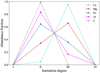 |
Fig. 9 Typical ionisation state of five elements in β Pic exocomets as constrained by the fit of our abundance measurements (Fig. 8) with Saha’s equation. |
5.5 Limitations
The main limitation of our abundance measurements is that they are very fragmented. Even though the number of studied species is rather large (12, including Fe II), these species were never observed altogether in one individual exocomet. In fact, most of the studied comets are generally observed in less than five different species simultaneously. This considerably limits our ability to study the variety of composition and ionisation states among β Pic exocomets, as we are still unable to build diagrams similar to Fig. 8 but for individual comets. In Sect. 5.4.2, Saha’s equation was thus fitted to the average abundance ratios measured across our comet sample (Table 2), providing rough constraints on the typical ionisation state of β Pic exocomets rather than on the properties of any individual object.
Some of our abundance measurements should also be taken with caution due to observing limitations. In particular, this is the case for abundance ratios derived from non-simultaneous observations (e.g. the Ca II/Fe II ratios), which may be affected by the time variation of the total amount of gas transiting the star. The different spectral resolutions of COS (R = 16 000–24 000) and STIS (R = 115 000) also make the estimate of the S II/Fe II ratio slightly hazardous, as cometary features observed in S II (with COS) are often blended. The curve of growth approach thus may not be the best tool to study exocomet absorption in S II. Here, a complete modelling of the cometary profile may be required.
It should also be noted that the assumption that the gas follows a Boltzmann distribution at T ~ 9000 K may not be valid for all the studied species. In particular, due to the very low stellar flux in the bottom of the Ca II H and K lines, the excitation of Ca II in the transiting comets may be fairly different than assumed by our model. Modelling the level population of Ca II in a similar way to that of Vrignaud & Lecavelier des Etangs (2024) and using radiative and collision coefficients from Meléndez et al. (2007), we calculated that ~87% of Ca II should remain in its ground state, compared to ~62% if the gas follows a Boltzmann distribution at 9000 K. Since our measurements are based on observations of the ground state of Ca II (through the H&K lines), the Ca II/Fe II ratios of the studied exocomets might be overestimated by as much as ~40%. Although the case of Ca II is probably special due to the extreme depth of the photospheric H and K lines, abundance measurements in other species may also be biased for this reason. Overcoming this issue would require complete modelling of the energy distribution of all the studied species, which is beyond the scope of the present work.
6 Conclusion
Our study provides the first abundance measurements of 12 ionised species in a large sample of exocomets that transited β Pic between 1997 and 2024. We found that the composition of the gaseous tails is fairly stable from one comet to another, particularly for singly ionised species (e.g. Ca II, Ni II, Cr II) and overall consistent with solar abundances. This validates the use of the curve of growth approach to study the composition of β Pic exocometary tails.
We showed that the typical abundances of refractory ions in β Pic exocomets is strongly correlated with ionisation energy, which indicates that ionisation plays a prominent role in the composition of these gaseous tails. For instance, Ca II, which is fairly easy to ionise (11.9 eV), is systematically depleted by a factor of about ten compared to Fe II (16.2 eV). A closer study of the measured abundances showed that Fe is generally split into similar fractions between Fe II and Fe III, while only ~4% of Ca is in the form of Ca II, the rest being Ca III. These estimates were confirmed by the fit of our abundance measurements with the Saha equation. A clear correlation between the Al III/Fe II ratio and the radial velocity was also noted. This indicates that the most redshifted comets are also more ionised, likely due to their closer distance to β Pic. These results could enable further studies of the ionisation processes in β Pic exocomets in order to quantify the relative contributions of potential mechanisms such as photoionisation, electron impact ionisation, or stellar wind charge exchange.
This first characterisation of the typical ionisation state in β Pic exocomets allows the ionisation state of other elements to be predicted, including tracers of volatiles (C, N, O). For instance, extrapolating the fitted law of Saha to carbon, we can estimate that the typical neutral fraction of C in β Pic exocomets is around 1–2%. This value, coupled with observations of exocomets in C I and Fe II lines (both accessible with STIS), could enable the determination of the C/Fe ratio of β Pic exocomets and yield valuable insight into their formation mechanisms.
However, our abundance measurements remain fragmented, as the number of detected species in each individual comet is generally too low to allow a case-by-case study of their ionisation state and composition. To overcome this lack of data, new observations of β Pic on a broader wavelength domain are required to allow for the detection of new exocomets in a large number of species simultaneously. Such observations will be obtained by 2025 with the HST program #17790 (Vrignaud et al. 2024b), which will target the whole wavelength domain between 1200 and 2900 Å at four different epochs. This program will allow for in-depth studies of the ionisation state in individual comets thanks to simultaneous observations of a large number of species with diverse ionisation potentials (e.g. S I, Mg II, Fe II, Ni II, S II). The C/Fe of the detected exocomets will also be inferred using measurements in C I and Fe II lines and estimates of the ionisation state in each object. The present paper thus serves as a benchmark for these future studies, demonstrating the relevance of abundance ratio measurements to probe the composition of β Pic exocomets and identify the physical processes that ionise the gas.
Data availability
Appendix G is available at: https://doi.org/10.5281/zenodo.15065712.
Acknowledgements
T.V. & A.L. acknowledge funding from the Centre National d’Études Spatiales (CNES).
Appendix A lonisation state
Let X be a given chemical element (Fe, Al, Ca). Assuming that X and Al are present in solar abundances in exocometary tails, and that most of the Aluminium gas is either singly or doubly ionised, we have
![$\[\frac{s_{\mathrm{X}}}{s_{\mathrm{Al}}}=\left[\frac{\mathrm{X}}{\mathrm{Al}}\right]_{\odot}=\frac{[\mathrm{X}]_{\mathrm{e}}}{[\mathrm{Al} \small~{\text{II}}]_{\mathrm{e}}+[\mathrm{Al} \small~{\text{III}}]_{\mathrm{e}}}=\frac{\left[\frac{\mathrm{X}}{\mathrm{X}\small~{\text{II}}}\right]_{\mathrm{e}}}{\left[\frac{\mathrm{Al}\small~{\text{II}}}{\mathrm{X}\small~{\text{II}}}\right]_{\mathrm{e}}+\left[\frac{\mathrm{Al}\small~{\text{III}}}{\mathrm{X}\small~{\text{II}}}\right]_{\mathrm{e}}},\]$](/articles/aa/full_html/2025/05/aa53568-24/aa53568-24-eq27.png)
![$\[\left[\frac{\mathrm{X}{\small~{\text{II}}}}{\mathrm{X}}\right]_{\mathrm{e}}=\frac{s_{\mathrm{Al}}}{s_{\mathrm{X}}} \cdot\left(\left[\frac{\mathrm{Al}{\small~{\text{II}}}}{\mathrm{X}{\small~{\text{II}}}}\right]_{\mathrm{e}}+\left[\frac{\mathrm{Al}{\small~{\text{III}}}}{\mathrm{X}{\small~{\text{II}}}}\right]_{\mathrm{e}}\right)^{-1},\]$](/articles/aa/full_html/2025/05/aa53568-24/aa53568-24-eq28.png)
where sAl = [Al/Fe]⊙ and sX = [X/Fe]⊙, and where the index e refers to exocometary abundances. Assuming that [X II/Fe II]e = ηX sX and [Al II/Fe II]e = ηAl sAl, with ηX and ηAl fixed values common to all exocomets (as found for singly ionised species, Fig. 5), we have
![$\[\left[\frac{\mathrm{Al} \small~{\text{II}}}{\mathrm{X}{\small~{\text{II}}}}\right]_{\mathrm{e}}=\frac{\eta_{\mathrm{Al}} s_{\mathrm{Al}}}{\eta_{\mathrm{X}} s_{\mathrm{X}}}, \quad\left[\frac{\mathrm{Al} \small~{\text{III}}}{\mathrm{X}{\small~{\text{II}}}}\right]_{\mathrm{e}}=\frac{1}{\eta_{\mathrm{X}} s_{\mathrm{X}}}\left[\frac{\mathrm{Al} \small~{\text{III}}}{\mathrm{Fe} \small~{\text{II} }}\right]_{\mathrm{e}},\]$](/articles/aa/full_html/2025/05/aa53568-24/aa53568-24-eq29.png)
![$\[\left[\frac{\mathrm{X}{\small~{\text{II}}}}{\mathrm{X}}\right]_{\mathrm{e}}=\left(\frac{\eta_{\mathrm{Al}}}{\eta_{\mathrm{X}}}+\frac{1}{\eta_{\mathrm{X}} s_{\mathrm{Al}}}\left[\frac{\mathrm{Al} \small~{\text{III}}}{\mathrm{Fe} \small~{\text{II}}}\right]_{\mathrm{e}}\right)^{-1}.\]$](/articles/aa/full_html/2025/05/aa53568-24/aa53568-24-eq30.png)
Provided that ηX can be estimated from measurements in many exocomets, Eq. A.1 allows us to convert the measured Al III/Fe II ratio of a given exocomet into its X II/X ratio. As an example, Fig. A.1 provides the Ca II/Ca, Fe II/Fe and Al II/Al ratios of our cometary exocomet sample (when the Al III/Fe II ratio could be measured), using η values of 0.081 for Ca, 1 for Fe and 1.5 for Al (Table 2).
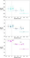 |
Fig. A.1 Estimates of the Ca II/Ca II(top), Fe II/Fe II (middle), and Al II/Al II(bottom) ratios of the studied exocomets, using Eq. A.1 and the measured Al III/Fe II ratios. Error bars reflect uncertainties on the measured Al III/Fe II ratios, and on the fixed parameters of Eq. A.1 (see Table 2). |
Appendix B Observations
Log of the 11 observations of β Pic from which our cometary sample was extracted. Other observations, not listed below, were used to reconstruct the EFS.
Appendix C Line examples
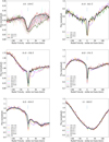 |
Fig. C.1 Examples of spectral lines used in our study. For conciseness, we show only one line for each series provided in Table F.1. We note that the Ca II doublet (3900 Å) was observed both by with HARPS (upper right) and MJUO (lower). |
Appendix D Comet list
The 29 comets studied in the present paper.
Appendix E Comet properties and composition
Fitted parameters of the cometary sample.
Measured composition of each studied exocomet.
Appendix F List of the studied lines
All spectral lines used in the study, grouped by series.
References
- Apai, D., Schneider, G., Grady, C. A., et al. 2015, ApJ, 800, 136 [NASA ADS] [CrossRef] [Google Scholar]
- Asplund, M., Grevesse, N., Sauval, A. J., & Scott, P. 2009, ARA&A, 47, 481 [NASA ADS] [CrossRef] [Google Scholar]
- Bergeson, S. D., & Lawler, J. E. 1993, ApJ, 414, L137 [NASA ADS] [CrossRef] [Google Scholar]
- Beust, H., & Morbidelli, A. 1996, Icarus, 120, 358 [NASA ADS] [CrossRef] [Google Scholar]
- Beust, H., & Tagger, M. 1993, Icarus, 106, 42 [NASA ADS] [CrossRef] [Google Scholar]
- Beust, H., Milli, J., Morbidelli, A., et al. 2024, A&A, 683, A89 [NASA ADS] [CrossRef] [EDP Sciences] [Google Scholar]
- Boissé, P., & Bergeron, J. 2019, A&A, 622, A140 [EDP Sciences] [Google Scholar]
- Chen, C. H., Lu, C. X., Worthen, K., et al. 2024, ApJ, 973, 139 [Google Scholar]
- Deleuil, M., Gry, C., Lagrange-Henri, A. M., et al. 1993, A&A, 267, 187 [NASA ADS] [Google Scholar]
- Ferlet, R., Hobbs, L. M., & Vidal-Madjar, A. 1987, A&A, 185, 267 [NASA ADS] [Google Scholar]
- Foreman-Mackey, D., Hogg, D. W., Lang, D., & Goodman, J. 2013, PASP, 125, 306 [Google Scholar]
- Gontcharov, G. A. 2007, VizieR Online Data Catalog: III/252 [Google Scholar]
- Gray, R. O., Corbally, C. J., Garrison, R. F., et al. 2006, AJ, 132, 161 [Google Scholar]
- Kiefer, F., Lecavelier des Etangs, A., Augereau, J. C., et al. 2014a, A&A, 561, L10 [NASA ADS] [CrossRef] [EDP Sciences] [Google Scholar]
- Kiefer, F., Lecavelier des Etangs, A., Boissier, J., et al. 2014b, Nature, 514, 462 [Google Scholar]
- Kramida, A., Yu. Ralchenko, Reader, J., & NIST ASD Team 2023, NIST Atomic Spectra Database (ver. 5.11), [Online]. Available: https://physics.nist.gov/asd [2023, December 15]. National Institute of Standards and Technology, Gaithersburg, MD [Google Scholar]
- Lagrange, A. M., Bonnefoy, M., Chauvin, G., et al. 2010, Science, 329, 57 [Google Scholar]
- Lagrange, A. M., Meunier, N., Rubini, P., et al. 2019, Nat. Astron., 3, 1135 [NASA ADS] [CrossRef] [Google Scholar]
- Lecavelier des Etangs, A., Cros, L., Hébrard, G., et al. 2022, Sci. Rep., 12, 5855 [NASA ADS] [CrossRef] [Google Scholar]
- Manfroid, J., Hutsemékers, D., & Jehin, E. 2021, Nature, 593, 372 [Google Scholar]
- Meléndez, M., Bautista, M. A., & Badnell, N. R. 2007, A&A, 469, 1203 [Google Scholar]
- Miret-Roig, N., Galli, P. A. B., Brandner, W., et al. 2020, A&A, 642, A179 [NASA ADS] [CrossRef] [EDP Sciences] [Google Scholar]
- Montgomery, S. L., & Welsh, B. Y. 2012, PASP, 124, 1042 [CrossRef] [Google Scholar]
- Nilsson, H., Ljung, G., Lundberg, H., & Nielsen, K. E. 2006, A&A, 445, 1165 [NASA ADS] [CrossRef] [EDP Sciences] [Google Scholar]
- Nowak, M., Lacour, S., Lagrange, A. M., et al. 2020, A&A, 642, L2 [NASA ADS] [CrossRef] [EDP Sciences] [Google Scholar]
- Rebollido, I., Eiroa, C., Montesinos, B., et al. 2020, A&A, 639, A11 [EDP Sciences] [Google Scholar]
- Rebollido, I., Stark, C. C., Kammerer, J., et al. 2024, AJ, 167, 69 [NASA ADS] [CrossRef] [Google Scholar]
- Roberge, A., Feldman, P. D., Weinberger, A. J., Deleuil, M., & Bouret, J.-C. 2006, Nature, 441, 724 [NASA ADS] [CrossRef] [Google Scholar]
- Smith, B. A., & Terrile, R. J. 1984, Science, 226, 1421 [Google Scholar]
- Strøm, P. A., Bodewits, D., Knight, M. M., et al. 2020, PASP, 132, 101001 [Google Scholar]
- Tobin, W., Barnes, S. I., Persson, S., & Pollard, K. R. 2019, MNRAS, 489, 574 [NASA ADS] [CrossRef] [Google Scholar]
- Vidal-Madjar, A., Hobbs, L. M., Ferlet, R., Gry, C., & Albert, C. E. 1986, A&A, 167, 325 [NASA ADS] [Google Scholar]
- Vidal-Madjar, A., Lagrange-Henri, A. M., Feldman, P. D., et al. 1994, A&A, 290, 245 [NASA ADS] [Google Scholar]
- Vrignaud, T., & Lecavelier des Etangs. 2024, A&A, 691, A2 [NASA ADS] [CrossRef] [EDP Sciences] [Google Scholar]
- Vrignaud, T., Lecavelier des Etangs, A., Kiefer, F., et al. 2024a, A&A, 684, A210 [NASA ADS] [CrossRef] [EDP Sciences] [Google Scholar]
- Vrignaud, T., Lecavelier des Etangs, A., Strom, P. A., et al. 2024b, The C/Fe and Dust-to-ice Ratios in Beta Pictoris Exocomets, HST Proposal. Cycle 32, ID. #17790 [Google Scholar]
- Zieba, S., Zwintz, K., Kenworthy, M. A., & Kennedy, G. M. 2019, A&A, 625, L13 [NASA ADS] [CrossRef] [EDP Sciences] [Google Scholar]
All Tables
Average abundances of 11 refractory species in β Pic exocomets compared to solar ratios.
Log of the 11 observations of β Pic from which our cometary sample was extracted. Other observations, not listed below, were used to reconstruct the EFS.
All Figures
|
Fig. 1 Illustration of the EFS recovery. Top: view of the Fe II 2728 Å line, showing clear spectral variations from one visit to another. Bottom: same line showing the calculated EFS. |
| In the text | |
|
Fig. 2 Recovery of a reference spectrum for comet #1 (1997-12-06, grey area) in the Al III 1862 Å line. Unlike other lines, we did not try to recover the EFS. Instead, a continuum is fitted to the observed spectrum (using a cubic spline algorithm), which corrects for the perturbation of broad, shallow exocomets, undetected in other lines. |
| In the text | |
|
Fig. 3 Cometary absorption observed in Fe II (top) and Ca II lines (middle, one hour later) on December 15, 2018. The EFS is plotted with a thick black line. The comparison of the absorption after division by the reference spectrum is given in the bottom panel (the region near the circumstellar line was removed due to a poorer EFS determination in Fe II lines). |
| In the text | |
|
Fig. 4 Zoomed-in view of the 2750.13 Å Fe II line (indicated with a solid blue marker). Even if cometary signatures are detected, they are blended with absorptions from other close Fe II lines at 2749.99 and 2750.30 Å (dotted markers). Due to this blending, the triplet was not included in our curve of growth analysis. |
| In the text | |
|
Fig. 5 Overview of all abundance measurements performed throughout the 29 exocomet sample, grouped by chemical species. For each species (e.g. S I), the measured ratios with Fe II were divided by the solar ratio of the corresponding elements (e.g. S/Fe), as given by Asplund et al. (2009). The ordering of the species reflect their ionisation energy. Each group of measurements is ordered according to the comet indexes (Table D.1). |
| In the text | |
|
Fig. 6 All Ca II/Fe II ratios measured in our exocometary sample as a function of the comet redshift. Horizontal error bars reflect the radial velocity extent of the cometary signatures. |
| In the text | |
|
Fig. 7 All Al III/Fe II ratios measured in our cometary sample as a function of the comet redshift. Horizontal error bars reflect the radial velocity extent of the cometary signatures. The two violet markers indicate the two comets with clear S I detections (see text). |
| In the text | |
|
Fig. 8 Typical abundances of 11 atoms and ions in β Pic exocomets relative to Fe II and normalised by solar abundances. The numerical values used to build this figure are provided in Table 2. Grey crosses indicate the best-fit model with Saha’s equation (see Sect. 5.4.2). |
| In the text | |
|
Fig. 9 Typical ionisation state of five elements in β Pic exocomets as constrained by the fit of our abundance measurements (Fig. 8) with Saha’s equation. |
| In the text | |
|
Fig. A.1 Estimates of the Ca II/Ca II(top), Fe II/Fe II (middle), and Al II/Al II(bottom) ratios of the studied exocomets, using Eq. A.1 and the measured Al III/Fe II ratios. Error bars reflect uncertainties on the measured Al III/Fe II ratios, and on the fixed parameters of Eq. A.1 (see Table 2). |
| In the text | |
|
Fig. C.1 Examples of spectral lines used in our study. For conciseness, we show only one line for each series provided in Table F.1. We note that the Ca II doublet (3900 Å) was observed both by with HARPS (upper right) and MJUO (lower). |
| In the text | |
Current usage metrics show cumulative count of Article Views (full-text article views including HTML views, PDF and ePub downloads, according to the available data) and Abstracts Views on Vision4Press platform.
Data correspond to usage on the plateform after 2015. The current usage metrics is available 48-96 hours after online publication and is updated daily on week days.
Initial download of the metrics may take a while.