| Issue |
A&A
Volume 621, January 2019
|
|
|---|---|---|
| Article Number | A117 | |
| Number of page(s) | 9 | |
| Section | Numerical methods and codes | |
| DOI | https://doi.org/10.1051/0004-6361/201834215 | |
| Published online | 17 January 2019 | |
Detectability of shape deformation in short-period exoplanets
1
Instituto de Astrofísica e Ciências do Espaço, Universidade do Porto, CAUP, Rua das Estrelas, 4150-762 Porto, Portugal
e-mail: tunde.akinsanmi@astro.up.pt
2
Departamento de Física e Astronomia, Faculdade de Ciências, Universidade do Porto, Rua do Campo Alegre, 4169-007
Porto, Portugal
3
Department of Physics, University of Coimbra, 3004-516
Coimbra, Portugal
4
CIDMA, Department of Physics, University of Aveiro, 3810-193
Aveiro, Portugal
5
ASD, IMCCE, Observatoire de Paris, PSL Université, Sorbonne Université, 77 av. Denfert-Rochereau, 75014
Paris, France
6
Astrophysics Group, Keele University, Staffordshire, ST5 5BG
UK
7
National Space Research and Development Agency, Airport Road, Abuja, Nigeria
Received:
10
September
2018
Accepted:
6
December
2018
Context. Short-period planets are influenced by the extreme tidal forces of their parent stars. These forces deform the planets causing them to attain nonspherical shapes. The nonspherical shapes, modeled here as triaxial ellipsoids, can have an impact on the observed transit light-curves and the parameters derived for these planets.
Aims. We investigate the detectability of tidal deformation in short-period planets from their transit light curves and the instrumental precision needed. We also aim to show how detecting planet deformation allows us to obtain an observational estimate of the second fluid Love number from the light curve, which provides valuable information about the internal structure of the planet.
Methods. We adopted a model to calculate the shape of a planet due to the external potentials acting on it and used this model to modify the ellc transit tool. We used the modified ellc to generate the transit light curve for a deformed planet. Our model is parameterized by the Love number; therefore, for a given light curve we can derive the value of the Love number that best matches the observations.
Results. We simulated the known cases of WASP-103b and WASP-121b which are expected to be highly deformed. Our analyses show that instrumental precision ≤50 ppm min−1 is required to reliably estimate the Love number and detect tidal deformation. This precision can be achieved for WASP-103b in ∼40 transits using the Hubble Space Telescope and in ∼300 transits using the forthcoming CHEOPS instrument. However, fewer transits will be required for short-period planets that may be found around bright stars in the TESS and PLATO survey missions. The unprecedented precisions expected from PLATO and JWST will permit the detection of shape deformation with a single transit observation. However, the effects of instrumental and astrophysical noise must be considered as they can increase the number of transits required to reach the 50 ppm min−1 detection limit. We also show that improper modeling of limb darkening can act to bury signals related to the shape of the planet, thereby leading us to infer sphericity for a deformed planet. Accurate determination of the limb darkening coefficients is therefore required to confirm planet deformation.
Key words: methods: analytical / techniques: photometric / planets and satellites: interiors
© ESO 2019
1. Introduction
The existence of planets with short-period orbits around their stars came as a surprise at the inception of exoplanet discoveries especially because the first case was a gas giant (Mayor & Queloz 1995) bearing no resemblance to the planet configuration in our solar system. Several of these planets have now been found as they represent some of the most easily detected planets using both the transit and radial velocity methods. Planets reach their final shapes having attained hydrostatic equilibrium from balancing gravitational, pressure, and other external forces acting on them. Planet shapes are often assumed to be spherical for simplicity but they are triaxial in reality. For very-short-period planets (P < 1 − 2 days), the close proximity to their stars exposes them to strong tidal forces which deforms them and increases the triaxiality of their equilibrium shapes. Contribution to deformation of a planet can also come from its rotation, making it oblate (Barnes & Fortney 2003).
Planet shape can have noticeable effects on the light curve obtained from transit observations (Seager & Hui 2002; Carter & Winn 2010a,b). Analysis of the transit light curve of a planet assuming planet sphericity allows for a spherical radius Rspr to be obtained. However, Leconte et al. (2011) showed that planet deformation due to tidal and rotational forces lowers the observed transit depth in comparison to a spherical planet. This causes an underestimation of the radius when sphericity is assumed in the transit light curve analysis of a deformed planet. Since the density of a planet is calculated from the assumed spherical radius, the obtained density will consequently be overestimated. Burton et al. (2014) therefore provided density corrections for some short-period planets expected to be tidally deformed based on the Roche approximation (Chandrasekhar 1969). Tidal deformation is particularly significant for planets orbiting close to their stellar Roche limits and a number of planets have been discovered to orbit so close to this limit that they are bordering on tidal disruption (e.g., Gillon et al. 2014; Delrez et al. 2016). For some of these planets, theoretical calculations have been done using the Roche model by Budaj (2011) to estimate the planet shape and correct the derived spherical radii and densities for the expected planet deformation (e.g., Southworth et al. 2015; Delrez et al. 2016). Correia (2014) formulated an analytical model for computing the shape of a deformed planet based on the fluid second Love number and also showed the difference between light curves of deformed and spherical planets.
Despite these efforts, there has been no observational detection of tidal deformation in short-period planets which would provide better estimates of their parameters. We therefore investigate the possibility of detecting deformation in the transit light curve of short-period planets with some current and near-future observational instruments. We modify the ellc transit tool by Maxted (2016)1 to incorporate the planet shape model by Correia (2014). The modified ellc is used to generate the light curve for a deformed planet based on its fluid second Love number. This allows us to obtain an estimate for the Love number of the planet that best matches the transit observations, which provides insights into the internal structure differentiation of the planet.
In Sect. 2, we summarize the model used to compute the shape of the planet and modification of the transit tool used to generate the light curves. In Sect. 3 we apply the modified tool to investigate the detectability of planet deformation in a case study of a known short-period planet. In Sect. 4, we discuss the results and some useful considerations for detecting planet deformation. We present our conclusions in the last section.
2. Modeling transit of deformed planets
2.1. Planet shape
Modeling the shape of a deformed planet follows the analytical formulation by Correia (2014) in which the planet is described by a triaxial ellipsoid centered at the origin of a Cartesian coordinate. As shown in Fig. 1, the semi-principal axes (a, b, c) of the ellipsoid are aligned with the X, Y, Z axes of the coordinate system, respectively. The equilibrium shape and mass distribution of a planet depends on the forces acting on it, namely the planet’s self gravity and other perturbing potentials. The planet can deform under the influence of centrifugal and tidal potentials. For a tidally locked close-in planet with circularized orbit of radius r0, Correia & Rodriguez (2013) give the nonspherical contribution from the perturbing potential on the surface of the planet as
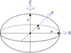 |
Fig. 1. Schematic of triaxial ellipsoid centered on the origin of the Cartesian coordinate system (X, Y, Z) with positive X-axis pointing towards the star. |
where G is the gravitational constant. The first term on the right-hand-side is the deformation contribution from the centrifugal potential resulting from the planet’s coplanar and synchronous rotation rate Ω about the Z-axis. The second term refers to the tidal contribution to the deformation along the X-axis by a star of mass M*.
Following Love (1911), Correia (2014) describes this deformation using a Love number approach such that the fluid second Love number for radial displacement hf is related to the radial deformation of the planet ΔR. The equilibrium surface deformation is thus given by
where g is the average surface gravity of the planet, and hf is a dimensionless quantity that quantifies the response (in terms of deformation) of a planet to a perturbing potential2. The magnitude of hf depends on the mass distribution of the planet. More homogeneous planets have higher hf whereas planets that are more centrally condensed have lower hf (Kramm et al. 2011, 2012). For an incompressible homogeneous planet, hf = 2.5 which is the theoretical maximum value (Leconte et al. 2011; Correia 2014). The physical values of hf range from 1 to 2.5 where hf = 1 would represent highly differentiated bodies with high core mass like FGK stars and hf = 2.5 is only possible for significantly homogeneous bodies like asteroids. In comparison, Jupiter has hf ≈ 1.5 and Earth has hf ≈ 2 (Yoder et al. 1995). A first observational measurement of the Love number of Saturn was recently obtained by Lainey et al. (2017) leading to a value of hf = 1.39 (from kf = 0.39).
Due to the synchronous rotation, the semi-principal axis a of the planet always points in the direction of the star leading to a tidal deformation along a. The shape of the planet is such that a > b > c and the deformation is kept constant along the circularized orbit. For the ellipsoid, we can define also the radius of a sphere that will enclose the same volume as the ellipsoid so that Rv = (abc)1/3. According to the formulation by Correia (2014), the semi-principal axes are related as a = b (1 + 3q) and c = b (1 − q). We can then write b as a function of Rv to first order in the parameter q as
so that
and
where q is an asymmetry parameter that relates to hf according to
The asymmetry parameter q quantifies the deformation of a planet, and is a measure of the difference between the semi-principal axes of the ellipsoid. Maximum deformation (hence maximum q) is attained for a given planet when it orbits at the Roche radius (r0 = rR = 2.46 Rv[M*/mp]1/3). Therefore, for maximum hf = 2.5, we have qmax ≃ 0.083. The equilibrium shape of a planet therefore depends on its radius, its fluid second Love number hf, the mass ratio between star and planet M*/mp, and also the distance from the planet to the star, r0. Figure 2 shows how tidal deformation becomes negligible with semi-major axis (in units of its Roche radii) for a given body with hf = 2.5 and again with Jupiter’s hf = 1.5. We see that far away from the star, irrespective of the value of hf, the planet does not deform (q ≃ 0) and so its shape remains largely spherical (a ≃ b ≃ c from Eqs. (3)–(5)). In general, Eq. (6) shows that tidal deformation is more relevant for large planets orbiting very close to their Roche radii. Planets with the highest absolute deformation (highest product q × Rv) provide the best chance to detect deformation.
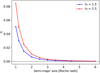 |
Fig. 2. Quantification of tidal deformation as a function of distance to the star for two different hf values. |
2.2. Transit model
Planetary features that change the shape of a planet (oblateness or rings) have the effect of modifying the transit light curves (e.g., Barnes & Fortney 2003; Akinsanmi et al. 2018). In the same vein, tidal deformation of a planet can modify the observed transit light curve. To model the transit of a deformed planet, the above ellipsoidal shape model by Correia (2014) was incorporated as a subroutine into a new version of the ellc transit tool by Maxted (2016). The ellc light curve model allows the projection of the ellipsoid and generation of the corresponding transit light curve. The projected shape of the ellipsoid on the stellar disk is an ellipse whose dimensions depend on the phase of the planet due to rotation of the ellipsoid with phase (see Fig. A.1 in Correia 2014). The rotation of the ellipsoid causes the cross-section of the planet to vary during transit. It should be noted that the shape correction model by Budaj (2011) does not account for the varying ellipsoidal cross-section during transit, thereby making ellc a more complete model involving this observational effect. Detailed descriptions of the ellc tool and the input parameters can be found in Maxted (2016).
The modified transit model, in addition to the usual transit parameters, takes the value of hf and the ellipsoid’s volumetric radius Rv as inputs. Therefore, by fitting the ellipsoidal model to the transit observation, all the parameters of the transit can be obtained, including the shape of the planet, and hf is estimated from the best fit of the model. Therefore, rather than obtaining the usual transit radius Rspr from spherical planet models, we obtain the best-match dimensions a, b, c of the ellipsoidal planet and calculate Rv.
2.3. The case of WASP-103b
To illustrate the output of ellc for an ellipsoidal planet, we take the case of WASP-103b, an ultra-short-period planet (P = 22.2 hr) reported to be bordering on tidal disruption (Gillon et al. 2014) making it an ideal candidate to detect deformation. Based on revised parameters by Southworth & Evans (2016), WASP-103b has an average radius of 1.596 RJup and mass of 1.47 MJup (Table 1). It orbits its star at a semi-major axis (r0) of 0.01979 AU and an inclination (inc) of 88.2°. It is assumed to be on the edge of tidal disruption due to its semi-major axis of only 1.13 times its Roche radius. Taking the quoted radius as the volumetric radius of the ellipsoid, Fig. 3 compares the spherical planet light curve for WASP-103b to its ellipsoidal counterparts with different hf values. It is seen that the light-curve of the ellipsoidal model changes noticeably for different values of hf and also compared to the spherical case. This is because the ellipsoidal planet projects only a small cross-section of its shape during the transit thereby leading to a lower transit depth when compared to the spherical planet. The mid-transit phase has the smallest ellipsoidal cross-section of  which is less than the cross-section
  if the planet were spherical. Therefore, if a spherical model is used to make a fit to the observation of an ellipsoidal planet, the spherical radius Rspr derived will be smaller than the actual volumetric radius Rv = (abc)1/3 of the ellipsoid (see Fig. 4). This is in agreement with the result from Leconte et al. (2011). Differences in transit depth as hf varies in Fig. 3 are due to the fact that higher hf for the same planet causes more deformation, which leads to even smaller projected cross-sectional area. In our code, we allow for a case where hf = 0 (although not physical) to imply no deformation for the planet so that the ellipsoidal planet model is equivalent to that of a spherical planet and they produce the same light-curve with Rv = Rspr. This is important for the analysis we perform in the following section and allows us to use the same model to explain both a deformed and a spherical planet. Maxted (2016) already showed that the spherical light curve of ellc is in agreement with other transit tools like BATMAN (Kreidberg 2015).
System parameters for WASP-103b.
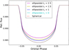 |
Fig. 3. Comparison of ellipsoidal model light curves of different hf values with spherical model light curve for WASP-103b. |
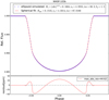 |
Fig. 4. Spherical fit to simulated deformed WASP-103b light curve. The bottom plot shows the residual representing the signature of deformation with amplitude quoted as the maximum absolute residual (max_abs_res). All length measurements are given in units of solar radii. |
2.4. Signature of deformation in transit light curves
Figure 1 in Correia (2014) showed difference plots between ellipsoidal and spherical light curves assuming both planets cover the same stellar area at the start of transit (full ingress). This perfectly captures the flux variation induced by deformation as both planets transit but is not the signature one would obtain from real observations, since the transit parameters would initially be unknown and would be determined from a fitting process. The observable signature of planet deformation is the residual between the light curve of the deformed planet and the best-fit spherical model. In Fig. 4, we simulated the light curve of deformed WASP-103b using our ellipsoidal model with parameters given in Table 1 and performed least-squares fitting using a spherical planet model. The residual from the fit is shown in the bottom panel and represents the signature of deformation for the simulated planet. The parameters derived from the fitting process are systematically incorrect as they adjust to mimic the signature of deformation. This also shows that the assumption of sphericity for a planet affects not only the radius derived but also the other transit parameters, and models that adjust only this radius are incomplete. We see in the residuals that the signature of deformation manifests in two regions. The first is at ingress and egress phases owing to oblateness (b > c) of the planet as identified in previous studies (e.g., Seager & Hui 2002; Barnes & Fortney 2003). A second prominent feature is seen as a bump centered on the mid-transit phase due to the varying star eclipsed area caused by ellipsoid rotation as it transits. This second feature is as a result of tidal deformation which was not accounted for in the previous studies mentioned but manisfests in our model due to full projection of the ellipsoidal shape as it rotates with phase (Correia 2014).
To compare the deformation signal obtained from the fitting process with the flux difference plot in Correia (2014), we perform spherical fits to the ellipsoidal simulation of other short-period giant planets WASP-19b, WASP-12b, WASP-4b, and WASP-121b that were presented in the study and were expected to be deformed. The residuals are shown in Fig. 5. We see from Figs. 4 and 5 that the amplitude of the deformation signature is just about 40 ppm for the most deformed planets (WASP-103b and WASP-121b) while the amplitudes from the difference curves in Correia (2014) are up to 100 ppm. We reiterate that the latter should not be taken to imply high signal detectability.
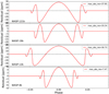 |
Fig. 5. Residuals from spherical fit to ellipsoidal simulations of different short-period planets in comparison to WASP-19b, 12b, and 4b from Correia (2014). |
WASP-103b, WASP-121b, and WASP-12b have the highest residual amplitudes and therefore present the best possibility of detecting deformation. Other planets likely to be deformed are HATS-18b, WASP-76b, and WASP-33b, but they have lower residual amplitudes of 20, 14, and 12 ppm, respectively.
3. Detectability of planet deformation and measurement of planet Love number
The residuals of the spherical fit to the light curve of a deformed planet is informative in detecting deformation as it shows that the spherical model does not fully explain the observation. However, some of the signature of the deformation is masked in the errors of the parameters obtained. To correctly estimate the planet transit parameters, our ellipsoidal model can be used to fit the transit observation. In doing so, we also obtain a value for the Love number that best fits the observation if there is enough precision in the data. The benefit of this approach is that we can fit the ellipsoidal model to any transit observation and, by the value of hf recovered, ascertain if planet deformation is detectable or not. If we cannot detect the deformation, we get hf ≈ 0 which as shown in Fig. 3 is equivalent to the fit of a spherical planet model.
Therefore, detectability of tidal deformation using the ellipsoidal model relies on the ability to recover a nonzero value of hf with statistical significance from a fitting process. Despite being able to infer deformation with only detection of hf ≫ 0, we will need to have hf ≥ 1 with some significance where the values give actual physical interpretation to astronomical bodies. To illustrate the detectability, we created simulated observations of deformed WASP-103b with one-minute cadence using its parameters as stated above with hf = 1.5. We used the Limb darkening toolkit (ldtk) by Parviainen & Aigrain (2015) to compute quadratic limb darkening coefficients of [0.5343, 0.1299] and their uncertainties [0.0012, 0.0027] in the CHEOPS bandpass for the star with stellar parameters given in Gillon et al. (2014). We added random Gaussian noise of different levels to the simulated data in each test run. We then investigated how well we can recover the value of hf and at what noise level it would be impossible to distinguish between the light curve of a spherical planet and that of a deformed planet. This is important to know the instrumental precision necessary to detect deformation in close-in planets.
We performed Markov Chain Monte Carlo (MCMC) analysis to estimate the transit parameters and their uncertainties using the emcee package (Foreman-Mackey et al. 2013) with uniform priors on hf in the range [0, 2.5]. As shown in Appendix A.1, when a noise level of 30 ppm is added to the simulated observation, hf is reliably recovered, with 99.7% of its samples (within ≃ ± 3σ) greater than 1. This proves that the result is statistically significant and implies that the planet is indeed deformed. Moreover, the residual from the fit does not show any structure related to the deformation signal. However, when a noise level of 100 ppm is added to the observation the median of the distribution suggests a deformed planet, but because its width encompasses hf = 0 (spherical model), planet deformation cannot be asserted (Appendix A.2). Figure 6 shows the detectability plot summarizing the results for the different noise levels added to the observation. We see that the significance of hf detection above 1 reduces as the noise level of the observation increases. For instance, at 50 ppm noise level, hf samples are well above zero, implying that the ellipsoidal model provides a better fit than the spherical model. However, the samples with hf < 1 do not represent physical values for a planet but the detection still gives ∼95% of the samples above 1. Beyond 50 ppm, fitting the observation with a spherical model becomes increasingly more probable. With noise levels as high as 100 ppm, the spherical and ellipsoidal models produce comparable fits.
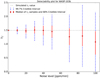 |
Fig. 6. Detectability of deformation in WASP-103b considering different noise levels. The black dashed line is the simulated hf value. The points are the median of the hf samples at each noise level. The red error bars show the 68% credible interval (≃ ± 1σ) while the blue error bars show the 99.7% credible interval (≃ ± 3σ). |
4. Discussion
The results show that noise levels below 30 ppm offer the best chance at detecting deformation for our test case of WASP-103b since we retrieve hf with ≥3σ significance above 1. However, we could define a lower limit on our detection confirmation such that we require to have (hf − 1σ)≥1 which puts 84% of the recovered hf samples in physical values expected for planets. This is satisfied for noise levels of 50 ppm and below.
A photometric precision of 50 ppm min−1 is not yet attainable using current observational instruments. For our case system, WASP-103 is a twelfth-magnitude star and the photometric precision to be attained by the near-future instrument CHEOPS for this star is 855 ppm min−1. Attaining a reduced photon noise level of 50 ppm min−1 for this star using CHEOPS requires ∼293 transit observations of WASP-103b. For the interesting candidate WASP-121b, which orbits its star of magnitude mV = 10 (Delrez et al. 2016), our analysis also showed detectability of deformation with 50 ppm min−1 noise level. CHEOPS precision for a tenth-magnitude star is 319 ppm min−1 thereby requiring only 40 transit observations to detect deformation in this planet. Although information from the CHEOPS consortium indicates that WASP-121 might not be in the visibility region, new interesting planet candidates with short period orbits may appear from future surveys targeting bright stars, such as PLATO (Rauer et al. 2014) and TESS (Ricker et al. 2015). For these planets around stars brighter than mV = 9, we expect photon noise levels as low as 150 ppm min−1 with CHEOPS (Broeg et al. 2013) and < 62 ppm min−1 with PLATO (Rauer et al. 2014) and thus require fewer transits to reach the 50 ppm limit needed to detect planet deformation as reported in Table 2. For these stars, TESS will have a relatively higher noise level of 464 ppm min−1 (Sullivan et al. 2015) which is not desirable for detecting deformation. Observations with the forthcoming JWST will also be immensely beneficial as it is expected to attain photon-noise floor ∼40 ppm (65 s) on its NIRCam instrument amongst others (Beichman et al. 2014). Attainment of this noise level implies that only one transit observation will be required in order to detect tidal deformation in a suitable short-period planet.
Number of transits required to reach 50 ppm min−1 noise level with CHEOPS and PLATO for different stellar magnitudes.
Unfortunately, interesting short-period planets expected to be significantly deformed were not found within the original Kepler survey field which would have allowed several transit observations of any found target. The WFC3 instrument on the Hubble Space Telescope (HST) achieved a noise level of 172 ppm (103 s) for two full-orbit observations of WASP-103 (Kreidberg et al. 2018). Therefore, with ∼40 transits of WASP-103b using HST, we can attain the required precision of 50 ppm min−1. However, some factors can still affect the detectability of deformation, some of which are mentioned below.
Temporal resolution. We used one-minute cadence in our simulations to enable good resolution of the ingress and egress phases which have short durations especially for these short-period planets. A lower cadence than this reduces the precision with which hf and other parameters are recovered. At the 30 ppm noise level, changing the cadence from 1 min to 4 mins and 8 mins increases the error on hf from ±0.12 to ±0.23 and ±0.38, respectively.
Orbital inclination. The inclination of the orbit plays a role in the signature of deformation. Lower inclinations indicate a shorter transit duration so the effects referred to in residuals of Fig. 4 and Sect. 2.4 will be shorter in time, making them more difficult to temporally resolve, especially at the ingress and egress phases. In addition, a longer transit duration allows the projected ellipse area to vary more (longer phase rotation of ellipsoid) making the light-curve more markedly different from that of the spherical planet thereby leading to a higher-amplitude bump around mid-transit (see also Fig. A.1 in Correia 2014). The effects of deformation in light curves is maximal at an inclination of 90° where hf is recovered with the best precision.
Limb darkening coefficients (LDCs). As shown in Fig. 4, the signature of deformation is prominent at ingress and egress phases with a bump centered around the mid-transit phase. The stellar limb-darkening affects light curves similarly in these regions (see effects of LDC modeling in Neilson et al. 2017), so we tested the impact of inaccurate estimation of limb-darkening coefficients on the recovery of hf from the light curve. This was attempted on the 30 ppm noise level simulation in two ways and the results are summarized in Table 3. First we fixed the limb darkening coefficients to incorrect values that are slightly different from the true values used to generate the simulated observation. We found that for incorrectly fixed LDC values that are smaller than the true values, the signature of deformation gets damped as we recover lower hf values than those simulated. When the values are fixed at values up to 0.01 smaller than the true values, the entire hf distribution falls around zero and we infer a spherical planet (see left plot in Fig. A.3). On the other hand, hf values are amplified when LDCs are fixed at values higher than the true values. For LDC values fixed at 0.015 higher than the true values, the recovered hf distribution is pushed towards the maximum of 2.5. In the latter case, we can infer that the planet is deformed but cannot ascertain the extent of deformation due to inaccurate estimation of hf which is evident from the obtained marginalized distribution (see right plot in Fig. A.3). The other attempt was to fit the LDCs by including them in the hyperparameters. We use a Gaussian prior with the true LDC values as mean and σ = 0.01. The MCMC sampling produced a wide hf distribution centered close to the true value but with errors as large as ±0.4 (left plot in Fig. A.4) making it difficult to ascertain planet shape. However, when tighter priors (e.g., using errors obtained from deriving LDCs with ldtk) are imposed on the LDCs, hf is well-recovered with errors of just ±0.18 to infer deformation (right plot in Fig. A.4). It should be noted that the LDC error estimates from ldtk are very small and have often had to be inflated in the literature during fitting to account for systematic errors in the atmospheric models (e.g., Raynard et al. 2018; Maxted & Hutcheon 2018).
Results of LDC tests and hf values recovered.
Alternatively, the power-2 limb darkening law has been recommended for the analysis of transit light curves as it has been shown to provide remarkable agreement between stellar atmospheric models and observations, particularly for cool stars (Morello et al. 2017; Maxted 2018). The transformation of the two parameters of the power-2 law in Maxted (2018) reduces the correlation between them during fitting and small errors of [0.011, 0.045] can be obtained on them. The fitting process can attempt different LDC laws so that the law with the best match to the observation and that produces the least errors on the derived parameters will be preferred.
Other noise sources. Our simulations considered the ideal situation where only photon (white) noise is present thereby allowing easy scaling of the noise with the number of observations/transits. However, in practice, other sources of noise (Pont et al. 2006) will impact the estimates given above and act to increase the number of transits required to detect deformation. These other noise sources can be from instrumental effects (e.g., satellite jitter and thermal instability) and also from astrophysical sources such as stellar activity (occulted or unocculted active regions; Oshagh et al. 2013), stellar oscillations and granulation (Chiavassa et al. 2017). These effects always have to be mitigated in transit analysis (Oshagh 2018; Barros et al. 2014) but will still impact the detectability of shape deformation. Recent developments in Gaussian process analysis also provide a method for tackling astrophysical noise (e.g., Foreman-Mackey et al. 2017; Serrano et al. 2018).
5. Conclusion
Short-period planets, especially within two Roche radii from the host star, suffer from extreme tidal forces causing their shapes to depart from sphericity in a way that is difficult to detect in transit observations. With the increasing observational precision of near-future instruments, detecting deformation becomes more feasible as planet shape will have a higher impact on the observed transit light curves. We demonstrate detectability of deformation for WASP-103b and WASP-121b (which have the highest deformation signatures as seen in Sect. 2.4 and are regarded as some of the most deformed planets; Delrez et al. 2016) by employing a formulation from the literature in a way that allows an observational estimate of a planet’s fluid Love number to be obtained. Because the Love number tells us how a planet deforms in response to perturbing potentials, we used it as a measure of deformation in the planet. Detecting and measuring planet deformation provides more accurate estimations of the radius and density of these planets as opposed to the estimates derived from spherical models or corrections calculated from only expectation of deformation. Additionally, measuring the Love number provides information about the interior structure of the planet. We showed that the instrumental precision needed to detect tidal deformation is ≤50 ppm which can be attained by CHEOPS with about 300 transits for WASP-103b and 40 transits for WASP-121b. The HST can also attain this precision for WASP-103b in approximately 40 transit observations. Fewer transit observations will be required if such short-period planets are found transiting very bright stars. Additionally, the precision expected from JWST will present the best opportunity to detect tidal deformation since only one transit of a suitable planet will be required.
The chances of detecting deformation are increased for planets with inclinations of 90° and also when the observations are taken with temporal resolution of ∼1 min. However detection can be severely hampered by improper modeling of the limb darkening which, in some cases, can cause the signature of deformation to be subdued, leading us to infer sphericity from the observations. Using the quadratic limb-darkening law, LDC errors smaller than 0.01 are required in order to confirm planet deformation. Proper treatment of noise sources will also be pertinent in order to identify the signature of shape deformation.
Available at https://pypi.org/project/ellc/
hf = 1 + kf where kf is the fluid second Love number for potential (Correia et al. 2014). Calculation of the different Love numbers can be found in Sabadini & Vermeersen (2004).
Acknowledgments
This work was supported by Fundação para a Ciência e a Tecnologia (FCT, Portugal) through national funds and by FEDER through COMPETE2020 by these grants UID/FIS/04434/2013 & UID/MAT/04106/2013 and POCI-01-0145-FEDER-007672 & PTDC/FIS-AST/1526/2014 & POCI-01-0145-FEDER-016886 & POCI-01-0145-FEDER-022217 & POCI-01-0145-FEDER-029932 & POCI-01-0145-FEDER-028953 &l POCI-01-0145-FEDER-032113. We also acknowledge support from FCT (Portugal) and POPH/FSE (EC) through fellowship PD/BD/128119/2016. NCS and SCCB also acknowledge support from FCT through Investigador FCT contracts IF/00169/2012/CP0150/CT0002 and IF/01312/2014/CP1215/CT0004 respectively. BA acknowledges support from FCT through the FCT PhD programme PD/BD/135226/2017. BA also thanks the LSSTC Data Science Fellowship Programme; his time as a fellow has benefited this work.
References
- Akinsanmi, B., Oshagh, M., Santos, N. C., & Barros, S. C. C. 2018, A&A, 609, A21 [NASA ADS] [CrossRef] [EDP Sciences] [Google Scholar]
- Barnes, J. W., & Fortney, J. J. 2003, ApJ, 588, 545 [NASA ADS] [CrossRef] [Google Scholar]
- Barros, S. C. C., Almenara, J. M., Deleuil, M., et al. 2014, A&A, 569, A74 [NASA ADS] [CrossRef] [EDP Sciences] [Google Scholar]
- Beichman, C., Benneke, B., Knutson, H., et al. 2014, PASP, 126, 1134 [NASA ADS] [CrossRef] [Google Scholar]
- Broeg, C., Fortier, A., Ehrenreich, D., et al. 2013, Eur. Phys. J. Web Conf., 47, 03005 [CrossRef] [EDP Sciences] [Google Scholar]
- Budaj, J. 2011, AJ, 141, 59 [NASA ADS] [CrossRef] [Google Scholar]
- Burton, J. R., Watson, C. A., Fitzsimmons, A., et al. 2014, ApJ, 789, 113 [NASA ADS] [CrossRef] [Google Scholar]
- Carter, J. A., & Winn, J. N. 2010a, ApJ, 716, 850 [NASA ADS] [CrossRef] [Google Scholar]
- Carter, J. A., & Winn, J. N. 2010b, ApJ, 709, 1219 [NASA ADS] [CrossRef] [Google Scholar]
- Chandrasekhar, S. 1969, Ellipsoidal figures of equilibrium (New Haven, London: Yale University Press) [Google Scholar]
- Chiavassa, A., Caldas, A., Selsis, F., et al. 2017, A&A, 597, A94 [NASA ADS] [CrossRef] [EDP Sciences] [Google Scholar]
- Correia, A. C. M. 2014, A&A, 570, L5 [NASA ADS] [CrossRef] [EDP Sciences] [Google Scholar]
- Correia, A. C. M., & Rodríguez, A. 2013, ApJ, 767, 128 [NASA ADS] [CrossRef] [Google Scholar]
- Correia, A. C. M., Boué, G., Laskar, J., & Rodríguez, A. 2014, A&A, 571, A50 [NASA ADS] [CrossRef] [EDP Sciences] [Google Scholar]
- Delrez, L., Santerne, A., Almenara, J.-M., et al. 2016, MNRAS, 458, 4025 [NASA ADS] [CrossRef] [Google Scholar]
- Foreman-Mackey, D., Hogg, D. W., Lang, D., & Goodman, J. 2013, PASP, 125, 306 [CrossRef] [Google Scholar]
- Foreman-Mackey, D., Agol, E., Ambikasaran, S., & Angus, R. 2017, AJ, 154, 220 [NASA ADS] [CrossRef] [Google Scholar]
- Gillon, M., Anderson, D. R., Collier-Cameron, A., et al. 2014, A&A, 562, L3 [NASA ADS] [CrossRef] [EDP Sciences] [Google Scholar]
- Kramm, U., Nettelmann, N., Redmer, R., & Stevenson, D. J. 2011, A&A, 528, A18 [NASA ADS] [CrossRef] [EDP Sciences] [Google Scholar]
- Kramm, U., Nettelmann, N., Fortney, J. J., Neuhäuser, R., & Redmer, R. 2012, A&A, 538, A146 [NASA ADS] [CrossRef] [EDP Sciences] [Google Scholar]
- Kreidberg, L. 2015, PASP, 127, 1161 [NASA ADS] [CrossRef] [Google Scholar]
- Kreidberg, L., Line, M. R., Parmentier, V., et al. 2018, AJ, 156, 17 [NASA ADS] [CrossRef] [Google Scholar]
- Lainey, V., Jacobson, R. A., Tajeddine, R., et al. 2017, Icarus, 281, 286 [NASA ADS] [CrossRef] [Google Scholar]
- Leconte, J., Lai, D., & Chabrier, G. 2011, A&A, 536, C1 [NASA ADS] [CrossRef] [EDP Sciences] [Google Scholar]
- Love, A. E. H. 1911, Some Problems of Geodynamics (Cambridge: Cambridge University Press) [Google Scholar]
- Maxted, P. F. L. 2016, A&A, 591, A111 [NASA ADS] [CrossRef] [EDP Sciences] [Google Scholar]
- Maxted, P. F. L. 2018, A&A, 616, A39 [NASA ADS] [CrossRef] [EDP Sciences] [Google Scholar]
- Maxted, P. F. L., & Hutcheon, R. J. 2018, A&A, 616, A38 [NASA ADS] [CrossRef] [EDP Sciences] [Google Scholar]
- Mayor, M., & Queloz, D. 1995, Nature, 378, 355 [NASA ADS] [CrossRef] [Google Scholar]
- Morello, G., Tsiaras, A., Howarth, I. D., & Homeier, D. 2017, AJ, 154, 111 [NASA ADS] [CrossRef] [Google Scholar]
- Neilson, H. R., McNeil, J. T., Ignace, R., & Lester, J. B. 2017, ApJ, 845, 65 [NASA ADS] [CrossRef] [Google Scholar]
- Oshagh, M. 2018, Asteroseismology and Exoplanets: Listening to the Stars and Searching for New Worlds, 49, 239 [NASA ADS] [CrossRef] [Google Scholar]
- Oshagh, M., Santos, N. C., Boisse, I., et al. 2013, A&A, 556, A19 [NASA ADS] [CrossRef] [EDP Sciences] [Google Scholar]
- Parviainen, H., & Aigrain, S. 2015, MNRAS, 453, 3821 [Google Scholar]
- Pont, F., Zucker, S., & Queloz, D. 2006, MNRAS, 373, 231 [NASA ADS] [CrossRef] [Google Scholar]
- Rauer, H., Catala, C., Aerts, C., et al. 2014, Exp. Astron., 38, 249 [NASA ADS] [CrossRef] [Google Scholar]
- Raynard, L., Goad, M. R., Gillen, E., et al. 2018, MNRAS, 481, 4960 [NASA ADS] [CrossRef] [Google Scholar]
- Ricker, G. R., Winn, J. N., Vanderspek, R., et al. 2015, J. Astron. Telesc. Instrum. Syst., 1, 014003 [NASA ADS] [CrossRef] [Google Scholar]
- Sabadini, R., & Vermeersen, B. 2004, Global Dynamics of the Earth: Applications of Normal Mode Relaxation Theory to Solid-Earth Geophysics (Dordrecht: Kluwer Academic Publishers) [Google Scholar]
- Seager, S., & Hui, L. 2002, ApJ, 574, 1004 [NASA ADS] [CrossRef] [Google Scholar]
- Serrano, L. M., Barros, S. C. C., Oshagh, M., et al. 2018, A&A, 611, A8 [NASA ADS] [CrossRef] [EDP Sciences] [Google Scholar]
- Southworth, J., & Evans, D. F. 2016, MNRAS, 463, 37 [NASA ADS] [CrossRef] [Google Scholar]
- Southworth, J., Mancini, L., Ciceri, S., et al. 2015, MNRAS, 447, 711 [NASA ADS] [CrossRef] [Google Scholar]
- Sullivan, P. W., Winn, J. N., Berta-Thompson, Z. K., et al. 2015, ApJ, 809, 77 [NASA ADS] [CrossRef] [Google Scholar]
- Yoder, C. F. 1995, in Global Earth Physics: A Handbook of Physical Constants, ed. T. J. Ahrens, 1 [Google Scholar]
Appendix A: Additional figures
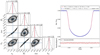 |
Fig. A.1. Left panel: posterior distributions for parameters of simulated deformed WASP103b with 30 ppm noise added. The values quoted on the diagonal histograms indicate the median marginalized distribution of each parameter (red lines) with the surrounding 68% credible interval (±1σ). The dashed vertical lines indicate the ±3σ limits calculated as the 0.15th and 99.87th percentiles. Blue lines indicate the true simulated values. Right panel: fit of simulated light curve of ellipsoidal WASP-103b with parameters retrieved from the sampling. |
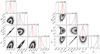 |
Fig. A.3. Left panel: as in Fig. A.1 but with LDCs fixed at incorrect values 0.01 smaller than the true values. Right panel: as in Fig. A.1 but with LDCs fixed at values 0.015 higher than the true values. |
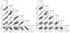 |
Fig. A.4. Left panel: posterior distributions of parameters when Gaussian prior with σ = 0.01 is used on the LDCs (u1, u2). Right panel: posterior distributions of parameters when tighter Gaussian priors from ldtk errors are used for the LDCs. |
All Tables
Number of transits required to reach 50 ppm min−1 noise level with CHEOPS and PLATO for different stellar magnitudes.
All Figures
|
Fig. 1. Schematic of triaxial ellipsoid centered on the origin of the Cartesian coordinate system (X, Y, Z) with positive X-axis pointing towards the star. |
| In the text | |
|
Fig. 2. Quantification of tidal deformation as a function of distance to the star for two different hf values. |
| In the text | |
|
Fig. 3. Comparison of ellipsoidal model light curves of different hf values with spherical model light curve for WASP-103b. |
| In the text | |
|
Fig. 4. Spherical fit to simulated deformed WASP-103b light curve. The bottom plot shows the residual representing the signature of deformation with amplitude quoted as the maximum absolute residual (max_abs_res). All length measurements are given in units of solar radii. |
| In the text | |
|
Fig. 5. Residuals from spherical fit to ellipsoidal simulations of different short-period planets in comparison to WASP-19b, 12b, and 4b from Correia (2014). |
| In the text | |
|
Fig. 6. Detectability of deformation in WASP-103b considering different noise levels. The black dashed line is the simulated hf value. The points are the median of the hf samples at each noise level. The red error bars show the 68% credible interval (≃ ± 1σ) while the blue error bars show the 99.7% credible interval (≃ ± 3σ). |
| In the text | |
|
Fig. A.1. Left panel: posterior distributions for parameters of simulated deformed WASP103b with 30 ppm noise added. The values quoted on the diagonal histograms indicate the median marginalized distribution of each parameter (red lines) with the surrounding 68% credible interval (±1σ). The dashed vertical lines indicate the ±3σ limits calculated as the 0.15th and 99.87th percentiles. Blue lines indicate the true simulated values. Right panel: fit of simulated light curve of ellipsoidal WASP-103b with parameters retrieved from the sampling. |
| In the text | |
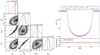 |
Fig. A.2. As in Fig. A.1 but with 100 ppm noise added to the simulated observation. |
| In the text | |
|
Fig. A.3. Left panel: as in Fig. A.1 but with LDCs fixed at incorrect values 0.01 smaller than the true values. Right panel: as in Fig. A.1 but with LDCs fixed at values 0.015 higher than the true values. |
| In the text | |
|
Fig. A.4. Left panel: posterior distributions of parameters when Gaussian prior with σ = 0.01 is used on the LDCs (u1, u2). Right panel: posterior distributions of parameters when tighter Gaussian priors from ldtk errors are used for the LDCs. |
| In the text | |
Current usage metrics show cumulative count of Article Views (full-text article views including HTML views, PDF and ePub downloads, according to the available data) and Abstracts Views on Vision4Press platform.
Data correspond to usage on the plateform after 2015. The current usage metrics is available 48-96 hours after online publication and is updated daily on week days.
Initial download of the metrics may take a while.