© ESO 2018

1. Introduction

Dark matter in the universe and stars in galaxies behave like a self-gravitating collisionless fluid of which the dynamics can be described by the Vlasov-Poisson system:

$$\begin{array}{cc}& {\displaystyle \frac{\partial f}{\partial t}}+\mathbf{v}·{\displaystyle \frac{\partial f}{\partial \mathbf{x}}}-{\displaystyle \frac{\partial \varphi }{\partial \mathbf{x}}}·{\displaystyle \frac{\partial f}{\partial \mathbf{v}}}=0,\hfill \end{array}$$(1)

$$\begin{array}{cc}& \mathrm{\Delta }\varphi =4\pi G\rho =4\pi G{\displaystyle \int f(\mathbf{x},\mathbf{v},t)}\mathrm{d}\mathbf{v},\hfill \end{array}$$(2)

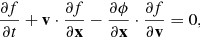
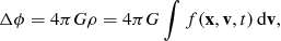
where f(x, v, t) is the phase-space density of the fluid at position x, velocity v, and time t, ρ is the mass density and ϕ is the gravitational potential.

A major issue when considering the dynamics of gravitational systems such as dark-matter halos, elliptical galaxies, or star clusters in the non-collisional regime is to understand the main processes underlying the creation of the quasi-stationary states that build up after a number of dynamical times, for instance the universal profiles of dark-matter halos (Navarro et al. 1996, 1997).

One way to relate initial to quasi-equilibrium state is to assume that the system reaches some maximum entropy state after a violent relaxation phase with strong mixing (Lynden-Bell 1967). However, the maximum entropy approach is at best partly successful (see, e.g. Yamashiro et al. 1992; Arad & Johansson 2005; Arad & Lynden-Bell 2005; Yamaguchi 2008; Joyce & Worrakitpoonpon 2011, and references therein) and the only way to improve the results is to introduce additional constraints and ad hoc ingredients (see, e.g. Hjorth & Williams 2010; Pontzen & Governato 2013; Carron & Szapudi 2013). Indeed, relaxation might be incomplete, or a maximum entropy state might not even exist, although one can generalise the concept of entropy by introducing H-functions (Tremaine et al. 1986), for which there exist stationary points related to actual stable equilibria even if an entropy maximum does not exist.

Another popular alternative method for understanding the establishment of quasi-stationary profiles consists in investigating the subspace of self-similar solutions (see, e.g. Fillmore & Goldreich 1984; Bertschinger 1985; Henriksen & Widrow 1995; Sikivie et al. 1997; Mohayaee & Shandarin 2006; Alard 2013, but this list is far from exhaustive). While it is difficult to actually demonstrate the onset of self-similarity, it seems to be a natural outcome of gravitational dynamics, at least in the absence of any characteristic scale. Although they exist as well in the warm case (see, e.g. Henriksen & Widrow 1995), self-similar solutions have been mostly studied in the cold case, for which the phase-space distribution function is of zero initial velocity dispersion. In this configuration, a D-dimensional phase-space sheet evolves in 2D phase-space and builds up a spiral pattern.

The above approaches, along with perturbation theory in cosmological systems (see, e.g. Bernardeau et al. 2002), provide some partial analytical framework to study the Vlasov-Poisson system. However, in general, these equations usually require a numerical approach, which consists in decomposing the phase-space distribution function on an ensemble of macro-particles interacting with one another with a softened gravitational force (see, e.g. Hockney & Eastwood 1988; Bertschinger 1998; Colombi 2001; Dolag et al. 2008; Dehnen & Read 2011, for reviews on the subject). An alternative way, easily tractable in a small number of dimensions or for systems with a high level of symmetry, consists in using direct Vlasov solvers where the phase-space distribution function is generally sampled on a Eulerian mesh. Most direct Vlasov solvers have been developed in plasma physics and are of semi-Lagrangian nature. They directly exploit Liouville theorem, namely that the phase-space density is constant along characteristics. In the standard semi-Lagrangian scheme, a test particle is associated to each grid site where f has to be calculated. This particle is followed back in time during a time-step and the value of f is given by the interpolation of the phase-space density at the previous time-step at the root of the trajectory. In the seminal implementation by Cheng et al. (1976), this is performed in a split fashion between velocities and positions. Many improvements and modifications have been added over time to the splitting algorithm of Cheng & Knorr (see, e.g. the extensive review in the introduction of Sousbie & Colombi 2016), mainly by plasma physicists. The splitting scheme was first applied to astrophysical systems by Fujiwara (1981), Nishida et al. (1981), and Watanabe et al. (1981). In the classical implementation that we use below, re-interpolation of the phase-space distribution function is performed at each time-step using a third-order spline.

In all the cases, validating the results obtained from numerical resolution of Vlasov-Poisson equations remains difficult, particularly if one aims to remain in the mean field limit. In particular, N-body results are often debated. For instance, the close N-body encounters and collective effects due to particle shot noise can have some dramatic, possibly cumulative effects (see, e.g. Aarseth et al. 1988; Kandrup & Smith 1991; Boily et al. 2002; Binney 2004; Joyce et al. 2009; Colombi et al. 2015; Beraldo e Silva et al. 2017; Romero & Ascasibar 2018), particularly when initial conditions are cold or close to cold (see, e.g. Melott et al. 1997; Melott 2007). While Vlasov codes do not use particles, they are still subject to non-trivial numerical effects, because a phase-space grid still remains a discrete representation of the system (see, e.g. Colombi et al. 2015; hereafter C15). But since the numerical implementation is still different from N-body codes, a comparison between Vlasov and N-body codes seems appropriate and timely, especially when trying to analyse in detail the quasi-stationary state reached in the fluid limit by gravitational systems.

One question indeed remains open. What are the main processes involved in the violent relaxation phase leading to a quasi-stationary state? We propose here to approach this question by studying the evolution of a number of initially spherical systems with various initial density profiles and velocity dispersions, focusing on the phase-space structure. Spherical symmetry allows us to compare high-resolution Vlasov simulations to N-body simulations. Our analyses focus on the detailed structure of the phase-space distribution function and comparisons with predictions from self-similarity.

The advantage of systems with initial spherical symmetry is that they have been studied in great detail in the literature both from the theoretical and the numerical points of view. One major question for instance concerns the role of radial instabilities and radial orbit instability in the establishment of the quasi-steady state observed after violent relaxation. Some spherical equilibria or quasi-steady states are known to be unstable to radial perturbations (see, e.g. Hénon 1973; Henriksen et al. 1997) as well as angular perturbations that translate into radial orbit instability as well studied in the literature (see, e.g. Polyachenko & Shukhman 1981; Merritt & Aguilar 1985; Barnes et al. 1986; Cannizzo & Hollister 1992; Barnes et al. 2009; Maréchal & Perez 2011; Vogelsberger et al. 2011; Polyachenko & Shukhman 2015). These perturbations are usually induced by shot noise due to the discrete nature of the distribution of stars or particles in the system, which directly relates to the discussion above about the validity of numerical simulations. Here, it is interesting to see what happens in the mean field limit, or at least in a regime that tries to approach it by using a direct Vlasov code and N-body simulations with a very large number of particles.

More specifically, assuming G = 1 and following the footsteps of Burkert (1990), Hozumi et al. (1996), and Hozumi et al. (2000), we perform a number of controlled numerical experiments of unity total mass systems, initially spherical with a power-law density profile and a Gaussian isotropic velocity dispersion:

$$\begin{array}{cc}& f(\mathbf{r},\mathbf{v})=\frac{{\rho }_0(r)}{{(2\pi {\sigma }_{\mathrm{r}}^2)}^{3/2}}exp(-\frac{1}{2}\frac{{\upsilon }^2}{{\sigma }_{\mathrm{r}}^2}),r\le R_0,\hfill \end{array}$$(3)

$$\begin{array}{c}\hfill {\rho }_0(r)\propto r^n,\end{array}$$(4)

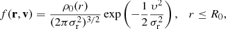
with R₀ = 2 being the initial radius of the sphere and the initial slope spanning the range n = 0 to n = −1.5. We consider “warm” and “cool” cases defined by their respective values of the virial ratio, η = 0.5 and 0.1, with

$$\begin{array}{c}\hfill \eta \equiv \frac{2T}{|W|},\end{array}$$(5)

where T is the total kinetic energy and W the total potential energy of the system.

In these simulations, we aim to study in detail the evolution of the phase-space distribution function, the onset of instabilities, and the consequence of these at the coarse-grained level. We also relate our measurements of fine details of the spiral pattern of the phase-space distribution to expectations from self-similar dynamics (see, e.g. Alard 2013; hereafter A13). To perform our simulations, we use three kinds of codes: a spherical semi-Lagrangian Vlasov solver, VlaSolve, presented in C15, the N-body public treecode Gadget-2 (Springel 2005), and a standard spherical shell N-body code (see, e.g. Hénon 1964). Importantly, while the systems are forced to remain spherical in VlaSolve and in the shell code, it is not the case for Gadget-2, which allows for the development of angular anisotropies. The variety of the codes employed in this work helps us to understand in detail the nature of different sources of instabilities, whether physical or numerical. In particular, we study the influence of finite spatial resolution in Vlasolve and of finite number of particles in the shell code and in Gadget-2.

This paper is organised as follows. In Sect. 2, we present the numerical codes used to perform the simulations and provide details on the various runs we performed. In Sect. 3, we perform a detailed visual inspection of the phase-space distribution function and discuss the various dynamical phases at play. Subsequently, Sect. 4 deals with self-similarity: we show how the calculations of A13 can be extended to spherical systems in a very simple way, and compare theoretical predictions on the shape of the phase-space distribution function to our numerical experiments. Finally, Sect. 5 summarises and discusses the results.

2. Simulations

In spherical symmetry, Vlasov equation can be written as

$$\begin{array}{c}\hfill \frac{\partial f}{\partial t}+{\upsilon }_{\mathrm{r}}\frac{\partial f}{\partial r}+(\frac{j^2}{r^3}-\frac{GM(<r)}{r^2})\frac{\partial f}{\partial {\upsilon }_{\mathrm{r}}}=0,\end{array}$$(6)

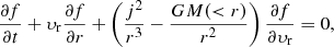
with r being the spherical radius, υ_r the radial velocity, j the conserved angular momentum and M(< r) the mass contained in a sphere of radius r. For a given value j, the evolution is therefore driven by the interplay between the gravitational force, dominating at large radii, and the centrifugal force j²/r³, dominating at small radii.

To solve Eq. (6), we have resorted to two numerical methods.

Firstly and mainly, we employ the spherical Vlasov solver VlaSolve presented in C15. This semi-Lagrangian code is similar to that of Fujiwara (1983) and thus uses the splitting algorithm of Cheng et al. (1976) to compute the evolution of the phase-space density on a mesh. The phase-space is divided into three-dimensional (3D) cells along radius, radial velocity, and angular momentum. A logarithmic scaling is used for radius to properly resolve the dynamics of the collapse at low radii, making the use of a minimum radius R_min necessary. To compute accurately the dynamics at low radii, the exact time spent by matter elements inside the sphere of radius R_min is computed assuming that gravitational force is negligible, which is an improvement over previous implementations which used the reflecting sphere method (see, e.g. Gott & Thuan 1976; Fujiwara 1983). More algorithmic details and tests of the code can be found in C15. Unless specified below, the grid for all the simulations is such that (N_r, N_v, N_j) = (2048, 2048, 128), where N_r is the number of vertices of radius in log scale, N_v is the number of vertices of radial velocity in linear scale, and N_j is the number of slices of angular momentum such that the kth slice contains fluid of angular momentum j_max((k−1/2)/N_j)², corresponding formally to the interval [j_max((k−1)/N_j)², j_max(k/N_j)²]. The computation domain is log₁₀ R_min ≡ −2 <  log₁₀(r)< 1.4, −υ_l <  υ_r <  υ_l and 0 <  j <  1.6, where υ_l = 2 for the runs with a virial ratio η = 0.5 and υ_l = 3 for the runs with a virial ratio η = 0.1. The limits are chosen such that almost all the mass of the system is contained in the computing domain during the simulated time, except for matter elements passing inside the sphere of radius R_min or those escaping from the system at large radius. For all the simulations, the time-step was chosen to be constant, equal to Δt = 0.005, a value larger than in C15 to avoid excessive diffusion due to over-frequent re-samplings of the phase-space distribution function, but we checked it is still on the safe side.

To avoid excessive aliasing effects in the VlaSolve runs, we apodize the initial profile given by Eq. (4) as follows,

$$\begin{array}{cc}& f(\mathbf{r},\mathbf{v})=\frac{{\rho }_0(r)}{{(2\pi {\sigma }_{\mathrm{r}}^2)}^{3/2}}exp(-\frac{1}{2}\frac{{\upsilon }^2}{{\sigma }_{\mathrm{r}}^2})\hfill \\ \hfill & \times \frac{1}{2}[1+\mathrm{erf}\left(\frac{R_0-r}{\mathrm{\Delta }}\right)],r\le R_0,\hfill \end{array}$$(7)

with Δ = 1/2, exactly as in C15. This apodization slightly changes the value of the virial ratio, of the order of 10% at most.

The second code we use relies on the standard spherical shells approach as in for example Hénon (1964) and Gott & Thuan (1976). We note that we employ it only for the most critical cases, namely (η, n) = (0.1, −1) and (η, n) = (0.1, −1.5), when the results from Gadget-2 differ too much from VlaSolve. In this N-body code, each particle represents a shell in configuration space and interacts with the other particles through gravitational force, −GM(< r)/r², which can be obtained very easily with a sorting procedure. The resolution of the Lagrangian equations of motion of the particles is performed simply with a leapfrog integrator with a constant time-step Δt = 0.001, five times smaller than the one chosen for the Vlasov code. Similarly as in Vlasolve, the Leapfrog algorithm is implemented using a decomposition of the Hamiltonian of the motion into a fully analytical drift part including centrifugal force and a kick part including solely gravitational force (see, e.g. Colombi et al. 2008). Initial shells distribution simply consists in taking the initial conditions of the Gadget-2 simulations described below, with the radius of each shell being equal to the magnitude of the position of each particle and their respective radial velocities and angular momenta directly derived from the three coordinates of the particle velocities.

Finally, we perform simulations using the public 3D N-body treecode Gadget-2 (Springel 2005) in its non-cosmological setup and with the treecode part only. The positions and velocities of particles are generated in a random way using a standard rejection method.

In the Gadget-2 simulations, spherical symmetry is no longer imposed, which leaves room for the development of angular anisotropies due to Poisson fluctuations in the initial particle distribution, even though the profile is initially spherical in the statistical sense. In particular, we see that the (η, n) = (0.1, −1) and (η, n) = (0.1, −1.5) simulations are subject to radial orbit instability. All the simulations in this work involved 10 million particles, except for one additional one performed with 100 million particles to examine the case (η, n) = (0.1, −1.5) more closely. The parameters for the Gadget-2 runs, in terms of softening length, force accuracy, and time-step control are otherwise the same as in C15.

Table 1 summarises the parameters used to perform the simulations of this work. In particular, the last two columns give the value of 25 t_dyn where

$$\begin{array}{c}\hfill t_{\mathrm{dyn}}=\sqrt{\frac{3\pi }{\rho }}\end{array}$$(8)

corresponds to the duration of a full radial orbit in a harmonic potential corresponding to a fixed density ρ. We estimate ρ from the simulations themselves, once the system has reached a quasi-stationary state, either directly at the centre of the system or as the average of the density in a sphere containing 10% of the total mass. Our estimates are rather crude but justify the choice of final time equal to 80 and 40 for the “warm” and “cool” cases, respectively. However, we must remain aware of the fact that increasing the magnitude of the slope |n| decreases the value of t_dyn.

3. Visual inspection: phase-space structure and density profiles

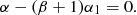
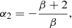
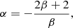
Figures 1 and 2 display, for a typical slice of fixed angular momentum, the phase-space distribution function of the “warm” and “cool” VlaSolve simulations, respectively. Additionally, Fig. 3 examines in more detail the case (η, n) = (0.1, −1.5), which is subject to radial orbit instability (ROI), while Fig. 4 provides projected density profiles. To supplement our discussion about ROI, we study in Fig. 5 the velocity anisotropy parameter for all the simulations as well as deviation from sphericity for the runs which experience ROI.

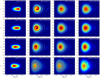Fig. 1. Snapshots of the phase-space density for the simulations with “warm” initial conditions, η ≃ 0.5. A typical slice of f(r, υr, j) with j = 0.16 is shown in (r, υr) space for the VlaSolve simulations at t = 0, at an early time t = 15, at an intermediate time used to perform tests of self-similarity of the phase-space spiral and at the final time.

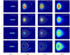Fig. 2. As in Fig. 1 but for the simulations with “cool” initial conditions, η ≃ 0.1 and for a slice with j = 0.06.

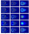Fig. 3. Closer examination of the onset of instabilities in phase space for the (η, n) = (0.1, −1.5) simulations: effects of spatial and mass resolutions. For the same angular momentum slice, j = 0.06, as in lower panels of Fig. 2, the phase space density is represented in (r, υr) space. The two first lines of panels correspond to two VlaSolve simulations with respective resolutions (Nr, Nv, Nj) = (2048, 2048, 128) and (1024, 512, 512). The next two lines of panels correspond to two Gadget-2 simulations with respective numbers of particles N = 107 and N = 108 and the last line of panels gives, for N = 107, the result obtained for the shell code. For the N-body simulations, the phase-space density is sampled on grids with resolution (Nr, Nv, Nj) = (1024, 1024, 32). One can notice that the phase-space sheet is less well defined or “fuzzier” in the N-body simulations than in the Vlasov code at low radius; this is because what is actually plotted is the distribution of particles (or shells) in a relatively large interval of angular momentum j ∈ [0.056, 0.077] to have sufficient number of particles to trace the phase-space distribution function, while for the Vlasov simulation, we selected only the slice corresponding to the value of j of interest. This figure illustrates the effect of radial instabilities and their dependence on spatial resolution (for the Vlasov code) or mass resolution (for the N-body code). We note the close agreement between the shell simulation and the Gadget-2 runs with 10 million particles in the middle panels of the third and fifth lines, while they diverge in the right panels when radial orbit instability effects become prominent in Gadget-2.

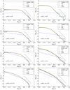Fig. 4. Radial density profile measured at various times in the VlaSolve simulations, namely initial conditions (blue dashes), intermediate time used to perform tests of self-similarity of the phase-space spiral (green), and final time (red dashes). For the final time, the results are also compared to a Gadget-2 run (thick grey), as well as the output of the shell code (thick grey dashes) for (η, n) = (0.1, −1) and (0.1, −1.5). In addition, the logarithmic slopes −4 and −2.1 (as measured in Hozumi et al. 2000) are shown respectively as a thin solid and a thin dashed line.

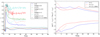Fig. 5. Velocity anisotropy and deviation from sphericity. Left panel: Velocity anisotropy parameter $\alpha =2\langle {\upsilon }_{\text{r}}^2\rangle /\langle {\upsilon }_{\perp }^2\rangle$ as a function of time for the VlaSolve (solid lines) and Gadget-2 simulations we performed (dashed curves). Right panel: Evolution of the departure from spherical symmetry for the two kind of initial conditions experiencing radial orbit instability in Gadget-2, namely (η, n) = (0.1, −1.0) (blue curves) and (η, n) = (0.1, −1.5) (red curves, solid and dashed for the 10 and 100 million particles simulations, respectively). The quantity $\mathrm{sgn}(1-{\mathrm{r}}_{\mathrm{axis}}){log}_{10}|1-{\mathrm{r}}_{\mathrm{axis}}|$ indicates the deviation from unity of raxis (in log scale and with a negative sign for raxis >  1), where raxis = b/c (upper curves) or b/a (lower curves), and a ≤ b ≤ c are the principal axis lengths of the Gadget-2 particle distribution derived from the inertia tensor.

Thanks to the high resolution of our simulations, when examining these figures, one can clearly separate, for the first time, two or three well-known dynamical phases, depending on initial conditions: (i) a violent relaxation phase during which the system converges to a quasi-steady state by building a very regular spiral structure in phase-space, (ii) a quiescent phase during which the quasi-steady state is preserved against small-scale radial instabilities which can destroy the spiral and (iii) relaxation to a non-spherical state through ROI when the system is prone to develop it. The novelty in our measurements is obviously not the discovery of the various phases of the dynamics, which are heavily discussed in the literature, but instead the clear articulation between them for the systems we study. We now discuss these three phases in detail.

3.1. Violent relaxation

In a first phase, the system undergoes violent relaxation that leads quickly to the establishment of a quasi-steady state. During this phase, spherical symmetry is preserved and the phase-space distribution function presents a very regular spiral structure in all cases, even in the N-body runs, thanks to the large number of particles we used to perform them. A movie of the evolution of the system shows that it is also subject to a global pulsation that introduces at some point irregular features in the phase-space distribution function in the outer parts of the spiral and at large radii, for example the dark region in upper-right panel of Fig. 1. During this violent relaxation phase, Gadget-2 agrees very well with VlaSolve, even in regions where these irregular features develop, as already noticed by C15 for the (η, n) = (0.5, 0) case, which shows that these features are intrinsic to the physical system and are not related to some additional instability due to some numerical noise.

3.2. Quasi-steady regime with small-scale radial instabilities

In a second phase, the system stays in quasi-equilibrium and preserves its spherical symmetry. However, some radial instabilities perturb it at small scales, irrespective of the numerical technique used, and can destroy the spiral structure. The time of the appearance of these instabilities is related to spatial resolution in the VlaSolve simulation and to the number of particles in the N-body simulations. This is well illustrated by Fig. 3 for (η, n) = (0.1, −1.5): for instance, increasing the number of angular momentum slices in the VlaSolve simulation reduces the magnitude of the perturbations of the spiral (compare middle insert of first and second line of panels), and similarly when increasing the number N of particles in the Gadget-2 runs (compare middle insert of third and fourth line of panels).

In the N-body case, these collective instabilities are induced by small, random but correlated errors on the gravitational force due to Poisson fluctuations in the particle distribution. In the VlaSolve code, they are related to coherent errors on the force due to the representation of the phase-space density on a grid, but the effect is analogous to the N-body case. These instabilities become naturally more significant when the initial velocity dispersion is reduced, as explained in C15. We also notice here that they take place earlier for larger |n|, in agreement with our calculation of dynamical times in the two right columns of Table 1. As a result, during the interval of time covered by our simulations, they can be seen in the cool runs and in the warm case for (η, n) = (0.5, −1.5), but they are not present or are negligible in other cases.

An important observation is that these instabilities intervene only at the fine level: they do not change the structure of the system at the coarse level, even quantitatively. To be more specific, if the phase-space density was smoothed at scales larger than the inter-filament separation – by filament, we mean for example some fold of the spiral structure – and larger than the size of the fluctuations introduced by radial instabilities, there would be no significant difference between late times, where these instabilities can destroy the spiral structure, and earlier times, when the spiral structure is still well defined. A good way to illustrate this consists in examining the projected density profile measured in the VlaSolve simulations, as displayed in Fig. 4, and to compare red curves to the green ones, which correspond to these aforementioned late and earlier times, respectively. The calculation of the projected density, by integrating the phase-space density over velocities, indeed corresponds to some coarse-graining procedure, although such anisotropic smoothing does not erase the quasi-caustic structures seen on the green curves of Fig. 4. These bumps correspond to projection of parts of the spiral (or any filament) that are orthogonal to configuration space. However, with proper (adaptive) smoothing at scales larger than the space between successive spiral folds, one can be convinced that agreement between the green curves and the red curves, already very good in most cases, should improve further.

The quasi-equilibrium built cinematically by the spiral is therefore stable against radial perturbations, but not necessarily the spiral structure.

3.3. Deviation from sphericity: radial orbit instability

In a third phase, small angular anisotropies induced by numerical noise become amplified through ROI for n ≤ −1 in the cool cases and the system deviates from spherical symmetry by acquiring a prolate shape (right panel of Fig. 5). A consequence of ROI is the reduction of the magnitude of the spherically averaged density profile ρ(r) at small radii, as can be seen in the two bottom-right panels of Fig. 4.

Radial orbit instability signature is best seen in the velocity anisotropy parameter

$$\begin{array}{c}\hfill \alpha =\frac{2⟨{\upsilon }_{\mathrm{r}}^2⟩}{⟨{\upsilon }_{\perp }^2⟩},\end{array}$$(9)

(see, e.g. Hozumi et al. 1996), where υ_r and υ_⊥ are respectively the radial and transverse velocities, as plotted in left panel of Fig. 5. Due to the dominant nature of radial infall during the very first phase of violent relaxation, cool initial conditions induce a strong velocity anisotropy, which is known, when exceeding some (still not fully known) threshold, to trigger ROIs in the presence of small perturbations to spherical symmetry (see, e.g. Polyachenko & Shukhman 1981; Merritt & Aguilar 1985; Barnes et al. 1986, 2009; Maréchal & Perez 2011; Polyachenko & Shukhman 2015, and references therein). In this case, the onset of ROI significantly reduces the value of α, as illustrated by the left panel of Fig. 5 for (η, n) = (0.1, −1) and (η, n) = (0.1, −1.5).

In our Gadget-2 simulations, small perturbations from spherical symmetry are related to shot noise, meaning that the onset of ROI is particle number dependent (see, e.g. Benhaiem et al. 2018), as illustrated in Fig. 5 by our two runs with 10 and 100 million particles in the (η, n) = (0.1, −1.5) case. On this figure, one also notices that ROI takes place later for n = −1 than for n = −1.5, but this is roughly consistent with the dynamical times given in the last two columns of Table 1.

The conditions of establishment of radial orbit instability are however not yet fully understood: some theoretical calculations and numerical experiments show that it should take place when α >  α_critical with α_critical ranging between 1 and 2.9 (see, e.g. Polyachenko & Shukhman 2015): this condition is clearly satisfied for (η, n) = (0.1, −1.0) and (0.1, −1.5) when examining the left panel of Fig. 5. Strictly speaking, given the limited amount of time we run the simulations, the other cases remain undecided even though we do not detect any ROI. The results obtained elsewhere in the literature, in particular by Merritt & Aguilar (1985), and Barnes et al. (2009), suggest that our “warm” systems are probably not prone to ROI, while, for (η, n) = (0.1, −0.5) and (η, n) = (0.1, 0), there is still a chance that ROI develops after some time. Clearly, our simulations are not run long enough to have all the details of the history of the system, which might evolve further to another interesting state.

Finally, we note that whether or not pure radial instability takes place before ROI is difficult to decipher from our simulations. Using linear analysis during collapse phase, Aarseth et al. (1988) argue that in the cold case, angular anisotropies introduced by Poisson noise are sub-dominant compared to radial ones, which suggests that a radial instability phase could take place before ROI. This argument is partly supported by Fig. 3, where excellent agreement is found between Gadget-2 and the spherical shell code at t = 4 (middle inserts of third and fifth lines of panels), when radial perturbations already significantly disrupt the phase-space spiral while ROI has not yet developed.

4. Self-similarity in phase space

In practice, seeking self-similar solutions to Vlasov-Poisson equations consists in finding solutions invariant with respect to some homothetic transforms, for example,

$$\begin{array}{c}\hfill f({\lambda }_1\mathbf{x},{\lambda }_2\mathbf{v},{\lambda }_{3}t)={\lambda }_{4}f(\mathbf{x},\mathbf{v},t),\end{array}$$(10)

which requires in this case f to be of the form of

$$\begin{array}{c}\hfill f(\mathbf{x},\mathbf{v},t)=t^{{\alpha }_0}F(\frac{\mathbf{x}}{t^{{\alpha }_1}},\frac{\mathbf{v}}{t^{{\alpha }_2}})·\end{array}$$(11)

Solving the Vlasov equation provides the solution for the function F. While a rigorous framework can be set to define self-similarity through Lie derivatives (Carter & Henriksen 1991), there is no unique way to express it. For instance, as studied in for example Henriksen & Widrow (1995), instead of Eq. (10), one can, in the spherically symmetric case, introduce anisotropy in the self-similar solution by separating the radial velocity from the angular momentum, or, in an extreme but well-known case, one can simply assume, as in the cold case, pure radial motions with zero angular momentum.

Strictly speaking, self-similarity implies a pure power-law behaviour for the projected density (see, e.g. Henriksen & Widrow 1995), which is obviously not the case for the systems we study here when examining Fig. 4, except to some extent at sufficiently large radii. However, self-similarity usually takes place only in a limited domain of phase-space. This can for instance simply be due to the finite extension of the system, which may induce deviations of the density profile from a pure power law, even though phase-space density is perfectly self similar. As a clear illustration of this statement, Alard (2013) argues that despite the cut-offs due to the finite nature of the system, local self-similarity in phase-space implies a power-law behaviour for the quantity Q(r) = ρ(r)/σ(r)³ where ρ(r) and σ(r) are respectively the projected density and the velocity dispersion, even if these latter are not found to be exact power laws of radius due to the cut-offs. Such a power-law property for Q(r) is verified to a great accuracy by dark-matter halos (see, e.g. Taylor & Navarro 2001), of which the density profiles are known to deviate from pure power laws (Navarro et al. 1996, 1997). As shown by Dehnen & McLaughlin (2005), solving the spherical Jeans equation assuming that Q(r) is a power law can indeed lead to non-pure power-law density profiles.

Here, we are clearly not in the case of a single self-similar regime (with possible cut-off effects). Indeed, for each value of the angular momentum j, our systems can trivially be separated into two distinct regions of phase space. In the first region, corresponding to a small-enough radius, the centrifugal acceleration j²/r³ dominates. Its power-law nature is expected to induce self-similarity in some domain of the considered phase-space slice. In the second region, corresponding to a large-enough radius, the gravitational acceleration −GM(< r)/r² dominates. Provided that it is also a power-law of radius, one expects another self-similar behavior. Given the discussion above about the possible effects due to the finite extent of the system, self-similar properties may be found even if the force is not exactly a power law. The transition between these two regions is sharp, as illustrated by Fig. 6, which is important to make our approach meaningful.

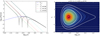Fig. 6. Small and large radii regimes in the (η, n) = (0.5, −1) VlaSolve run at t = 40. Left panel: plots separately the magnitude of centrifugal force j2/r3 and of the gravitational force as functions of radius as well as the magnitude of the sum of both forces. Right panel: isocontours of the specific energy (white curves) superposed on the phase-space distribution function for j = 0.16. In addition, the white dashes and dot-dashes assume that only the gravitational or the centrifugal force contributes, respectively.

Self-similarity also predicts the formation of a spiral in phase-space, of which the structure is defined by the self-similar parameters (see, e.g. Fillmore & Goldreich 1984, A13). We note, as already mentioned, that the onset of self-similarity does not require the assumption of cold initial conditions as is often supposed. For instance, in the calculations of A13, no such hypothesis is made, and the existence of a spiral structure in phase space is clearly seen when assuming self-similarity. Here, we cannot rigorously demonstrate the existence of such a spiral structure but can postulate it, predict its local properties in each of the supposed self-similar regimes mentioned above, and compare the predictions to our simulation measurements, which we do below, closely following Alard (2013; and priv. comm.).

When examining a slice of fixed angular momentum, we notice that the Vlasov equation for a spherical system is exactly analogous to the 1D case:

$$\begin{array}{c}\hfill \frac{\partial f}{\partial t}+{\upsilon }_{\mathrm{r}}\frac{\partial f}{\partial r}-\frac{\partial \psi }{\partial r}\frac{\partial f}{\partial {\upsilon }_{\mathrm{r}}}=0,\end{array}$$(12)

except that the force is derived from the following scalar field

$$\begin{array}{c}\hfill \psi (r)=\frac{j^2}{2r^2}+\varphi (r),\end{array}$$(13)

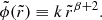
where ϕ(r) is the gravitational potential. A13 derived detailed self-similar solutions in the 1D case that we extend below in the regimes where the centrifugal force dominates ψ(r)≃j²/(2r²) and in the regime where gravitational potential dominates and is a power law, ψ(r)≃ϕ(r)∝r^β + 2.

Assuming that the conserved angular momentum j is a dummy variable, the self-similar solution for the phase-space distribution function can be expressed as follows:

$$\begin{array}{c}\hfill f(r,{\upsilon }_{\mathrm{r}},j,t)=t^{{\alpha }_0}{F}_j(\frac{r}{t^{{\alpha }_1}},\frac{{\upsilon }_{\mathrm{r}}}{t^{{\alpha }_2}})·\end{array}$$(14)

Setting

$$\begin{array}{c}\hfill \stackrel{\sim }{r}=\frac{r}{t^{{\alpha }_1}},\stackrel{\sim }{\upsilon }=\frac{{\upsilon }_{\mathrm{r}}}{t^{{\alpha }_2}},\end{array}$$(15)

we can express both the gravitational and the centrifugal force as functions of these new variables.

Starting from the gravitational force, we define a function U such that

$$\begin{array}{c}\hfill -\frac{\partial \varphi }{\partial r}\equiv t^{\alpha }U(\stackrel{\sim }{r}),\end{array}$$(16)

and we assume that

$$\begin{array}{c}\hfill U=-\mathrm{d}\stackrel{\sim }{\varphi }/\mathrm{d}\stackrel{\sim }{r},\end{array}$$(17)

with

$$\begin{array}{c}\hfill \stackrel{\sim }{\varphi }(\stackrel{\sim }{r})\equiv k{\stackrel{\sim }{r}}^{\beta +2}.\end{array}$$(18)

Then,

$$\begin{array}{c}\hfill U(\stackrel{\sim }{r})=-k(\beta +2){\stackrel{\sim }{r}}^{\beta +1},\end{array}$$(19)

and we obtain, from the Poisson equation,

$$\begin{array}{c}\hfill U(\stackrel{\sim }{r})=-\frac{G}{{\stackrel{\sim }{r}}^2}{\displaystyle {\int }_{{\stackrel{\sim }{r}}^{\prime }<\stackrel{\sim }{r}}8{\pi }^2{F}_j({\stackrel{\sim }{r}}^{\prime },\stackrel{\sim }{\upsilon })}\mathrm{d}{\stackrel{\sim }{r}}^{\prime }\mathrm{d}\stackrel{\sim }{\upsilon }j\mathrm{d}j,\end{array}$$(20)

$$\begin{array}{c}\hfill \alpha ={\alpha }_0+{\alpha }_2-{\alpha }_1.\end{array}$$(21)

Similarly, the centrifugal force can be written

$$\begin{array}{c}\hfill \frac{j^2}{r^3}\equiv t^{\alpha }U(\stackrel{\sim }{r}),\end{array}$$(22)

which implies

$$\begin{array}{c}\hfill \alpha =-3{\alpha }_1,\end{array}$$(23)

and, if we assume again that 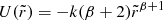$U(\stackrel{\sim }{r})=-k(\beta +2){\stackrel{\sim }{r}}^{\beta +1}$, we obtain

$$\begin{array}{c}\hfill \beta =-4,\end{array}$$(24)

$$\begin{array}{c}\hfill k=\frac{j^2}{2}·\end{array}$$(25)

By injecting these various expressions in the Vlasov equation in a regime where either the gravitational or centrifugal force dominates, one obtains

$$\begin{array}{cc}\hfill {\alpha }_0{F}_j& \hfill +\frac{\partial F_j}{\partial \stackrel{\sim }{r}}[-{\alpha }_1\stackrel{\sim }{r}+\stackrel{\sim }{\upsilon }{t}^{{\alpha }_2-{\alpha }_1+1}]\hfill \\ \hfill & \hfill +\frac{\partial F_j}{\partial \stackrel{\sim }{\upsilon }}[-{\alpha }_2\stackrel{\sim }{\upsilon }-k(\beta +2){\stackrel{\sim }{r}}^{\beta +1}{t}^{\alpha -{\alpha }_2+1}]=0.\hfill \end{array}$$(26)

Eliminating time dependence in this equation imposes

$$\begin{array}{cc}\hfill {\alpha }_1& \hfill ={\alpha }_2+1,\hfill \end{array}$$(27)

$$\begin{array}{cc}\hfill \alpha & \hfill ={\alpha }_2-1.\hfill \end{array}$$(28)

Enforcing stationarity of the force t^αU(r/t^α₁) with the power-law (19) implies

$$\begin{array}{c}\hfill \alpha -(\beta +1){\alpha }_1=0.\end{array}$$(29)

Hence the only viable solution is

$$\begin{array}{c}\hfill {\alpha }_2=-\frac{\beta +2}{\beta },\end{array}$$(30)

$$\begin{array}{c}\hfill {\alpha }_1=-\frac{2}{\beta },\end{array}$$(31)

$$\begin{array}{c}\hfill \alpha =-\frac{2\beta +2}{\beta },\end{array}$$(32)

which is of course consistent with Eq. (23) and leaves α₀ as a free parameter if the centrifugal force dominates; while if the gravitational force dominates, it fixes α₀ = −(β + 2)/β. We note that, in general, total mass is not conserved. Indeed, enforcing total mass conservation (or mass conservation per angular momentum slice, as well) imposes α₀ + α₁ + α₂ = 0, a condition which is fulfilled only for β = −3/2 and in this case α₀ = 1/3. This is not a problem because self-similarity is expected to take place only in a finite dynamical range.

To follow the notations of A13 as closely as possible, we now make the following change of variables,

$$\begin{array}{cc}\hfill \mathcal{G}& \hfill \equiv ln{F}_j,\hfill \end{array}$$(33)

$$\begin{array}{cc}\hfill \eta & \hfill \equiv \frac{\beta }{2}+1,\hfill \end{array}$$(34)

$$\begin{array}{cc}\hfill u& \hfill \equiv {\stackrel{\sim }{r}}^{\eta }.\hfill \end{array}$$(35)

Equation (26) becomes

$$\begin{array}{cc}\hfill -{\alpha }_0& \hfill +(1+{\alpha }_2)\eta \frac{\partial \mathcal{G}}{\partial u}u+{\alpha }_2\frac{\partial \mathcal{G}}{\partial \stackrel{\sim }{\upsilon }}\stackrel{\sim }{\upsilon }\hfill \\ \hfill & \hfill -\eta [\frac{\partial \mathcal{G}}{\partial u}\stackrel{\sim }{\upsilon }-2ku\frac{\partial G}{\partial \stackrel{\sim }{\upsilon }}]u^{\beta /(\beta +2)}=0,\hfill \end{array}$$(36)

which is exactly the same equation as Eq. (11) of A13, except that the first term α₂ + 2 is replaced here with −α₀. Hence, the solution of this equation is very similar to the expressions given in A13. The main difference here is that the values of β we consider are outside the domain of validity of the calculations of A13, which implies that the isocontours of the solutions are closer to hyperbolic curves than to a spiral. Here, however, we have to take into account the fact that we have two distinct supposed self-similar regimes, one dominated by centrifugal force, say for r ≲ r_crit(j), and the other dominated by gravitational force, say for r ≳ r_crit(j). Hence, the actual solution is the connection between too partial solutions following self-similar properties.

Rescaling variable $\stackrel{\sim }{r}$ so that k = 1/2 in Eq. (18), and introducing, exactly as in A13, the new variables

$$\begin{array}{cc}& \hfill R=\sqrt{u^2+{\stackrel{\sim }{\upsilon }}^2},\hfill \end{array}$$(37)

$$\begin{array}{cc}& \hfill cos\mathrm{\Psi }=\frac{u}{R},\hfill \end{array}$$(38)

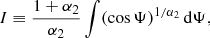
we obtain nearly exactly Eq. (12) of A13, but the parameters of this equation change according to whether the value of R cos Ψ is above or below a threshold fixed by r_crit. With $H(R,\mathrm{\Psi })\equiv G(u,\stackrel{\sim }{\upsilon })$ we write, following exactly the footsteps of A13, the general solution for H when the power-law force is stationary,

$$\begin{array}{c}H(R,\mathrm{\Psi })=\frac{{\alpha }_0}{{\alpha }_2}lnR\\ \hfill +Q(R^{-1/{\alpha }_2}+\frac{1+{\alpha }_2}{{\alpha }_2}{\displaystyle \int {(cos\mathrm{\Psi })}^{1/{\alpha }_2}}\mathrm{d}\mathrm{\Psi }),\end{array}$$(39)

with Ψ ∈ ] − π/2, π/2[ and where Q is some function. At this point, introducing the same concept of spiral as in A13 is not simple, because u >  0 does not allow Ψ to make a full excursion on the circle. Furthermore, the values of the logarithmic density profile slope β that we have to consider range in the interval −4 ≲ β <  −2, which implies, from Eq. (30), −1/2 ≲ α₂ <  0, hence some divergence of the integral

$$\begin{array}{c}\hfill I\equiv \frac{1+{\alpha }_2}{{\alpha }_2}{\displaystyle \int {(cos\mathrm{\Psi })}^{1/{\alpha }_2}}\mathrm{d}\mathrm{\Psi },\end{array}$$(40)

when |Ψ| approaches π/2. This is however not a real problem, because the objective is to connect two self-similar solutions. Here, we are unable to demonstrate the existence of the spiral structure in phase-space; we must postulate it. We therefore define a new angular variable θ and

$$\begin{array}{c}\hfill I(\theta )\equiv {\displaystyle \int g({\theta }^{\prime })}\mathrm{d}{\theta }^{\prime },\end{array}$$(41)

where g(θ) is a function with period 2π verifying

$$\begin{array}{cc}\hfill g(\theta )& \hfill \simeq g_{-}(\theta )\equiv \frac{1+{\alpha }_2^{-}}{{\alpha }_2^{-}}{[cos({\mathrm{\Psi }}^{-}=\theta -2k\pi )]}^{1/{\alpha }_2^{-}},\hfill \\ \hfill & \hfill \theta -2k\pi \simeq 0,\hfill \end{array}$$(42)

$$\begin{array}{cc}\hfill g(\theta )& \hfill \simeq g_{+}(\theta )\equiv \frac{1+{\alpha }_2^{+}}{{\alpha }_2^{+}}{[-cos({\mathrm{\Psi }}^{+}=\theta -2k\pi )]}^{1/{\alpha }_2^{+}},\hfill \\ \hfill & \hfill \theta -2k\pi \simeq \pi ,\hfill \end{array}$$(43)

and the symbols − and + correspond to the regimes dominated by the centrifugal and the gravitational force, respectively. Function g(θ) makes a smooth transition between g₋ and g₊. The only, trivial but important fact we have to know is that I(θ) defined this way is roughly proportional to θ which allows us now to explicitly define the concept of a spiral across both self-similar domains. Interestingly, the subsequent calculations of A13 are not changed at all when taking this new definition of I, and Eq. (19) of A13 still stands in each self-similar domain, with $I_1={\int }_0^{2\pi }g(\theta \prime )\hspace{0.17em}\text{d}\theta \prime$ now an unknown constant instead of a well-defined integral as in A13.

Therefore, in the situation where there are many folds, we have the following expected relationship for the interfold distance in each self-similar region:

$$\begin{array}{c}\hfill \mathrm{d}R\propto R^{1+1/{\alpha }_2}.\end{array}$$(44)

In particular, coming back to standard variables (r, υ_r), the interfold distances along the axis υ_r = 0 read

$$\begin{array}{c}\hfill \mathrm{d}r\propto r^{1-\beta /2}.\end{array}$$(45)

To test this property directly, we analyse, at a time where the spiral structure is still well defined, the function f(r, υ_r = 0, j) for a fixed value of angular momentum, as illustrated by Fig. 7. We determine the positions of the folds using local parabolic fits. For each fold i, we determine two semi-height radial positions log(r_l, i) and log(r_r, i) (the computational grid being logarithmic in radius) on the left and right of the peak, respectively, and define the error on the position of the peak as δlog(r_i) = log(r_r, i)−log(r_l, i).

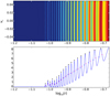Fig. 7. Illustration of the method used to determine the positions of the folds and corresponding interfold distance law at small radius in a phase-space slice. Top panel: zoom performed around the axis υr = 0 in the region dominated by centrifugal force for the (η, n) = (0.5, −1.0) simulation at t = 40. The corresponding phase-space distribution function f(r, υr = 0, j = 0.16) is plotted in the lower panel. The black dots give the positions of local maxima estimated with our local quadratic fit, while the blue and red dots provide upper and lower bounds to compute the (very conservative) error bars shown on Fig. 8.

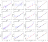Fig. 8. Interfold distance at null radial velocity vs. self-similar predictions for a fixed value of angular momentum. The distance dr between local maxima of the function f(r, υr = 0, j) is plotted as a function of r for the VlaSolve runs with various initial conditions. The time considered corresponds to the middle column of panels in Figs. 1 and 2. The two left columns of panels correspond to the “warm” case, η = 0.5 with j = 0.16, and the two right ones to the “cool” case, η = 0.1 with j = 0.06. Then, odd column numbers (1 and 3) and even column numbers (2 and 4) correspond to the regime where centrifugal/gravitational force dominates, respectively. On each panel a red line indicates the logarithmic slope predicted by self-similarity. When the gravitational force dominates, two additional dashed curves provide a bracket of the estimated slope taking into account deviations from self-similarity, i.e. variations of the effective logarithmic slope of the gravitational force.

Figure 8 summarises the results of our measurements in the VlaSolve simulations. At a “small” radius, the system is dominated by the centrifugal force, β = −4, hence dr ∝ r³. This prediction is compared to measurements in the simulations in the first and third columns of Fig. 8, which correspond to the simulations with “warm” and “cool” initial conditions, respectively. At a large enough radius, where the system is dominated by gravity, the force is only approximately a power law but an average slope can nevertheless be inferred in some interval of scales E_grav, corresponding to the regime where the gravitational force remains at least ten times larger than the centrifugal force and for r smaller than the turnaround radius. In the second and fourth columns of panels of Fig. 8, the slope of the red line is given by the corresponding value of 1 − β/2. There are also two dashed cyan and green lines corresponding to the minimum and maximum value of β found in E_grav, which gives an idea of deviation from a pure power law. Globally, the simulations agree rather well with self-similar predictions, except maybe at very small r in the first and third columns of panels of Fig. 8 and in the top panel of the second column in the same figure. We note however that measurements of the interfold distance for small values of r might be partly spurious, because we are in a regime where the phase-space distribution function is small and can be affected by aliasing. Also, we note that the spiral structure survives only a short time for (η, n) = (0.1, −1.5) which leaves only a small number of folds to deal with. Nevertheless, the agreement with self-similarity remains good when taking into account the limitations found in all the cases at very small r, already after only a few dynamical times.

Another interesting property than can be derived directly from Eq. (39) is the local shape of the spiral near the axis υ_r = 0, hence Ψ ≃ 0, and for small r, hence small R. Following the unnumbered equation after Eq. (16) of A13 and taking into account the fact that α₂ <  0, we expect an isocontour of the function H(R, Ψ) to have the following shape in the regime R ≪ 1, Ψ ≃ 0,

$$\begin{array}{c}\hfill R\propto {\mathrm{\Psi }}^{-{\alpha }_2}\propto {\mathrm{\Psi }}^{(\beta +2)/\beta }.\end{array}$$(46)

We note therefore that because of the form of the interfold law (44), the spiral actually locally coincides with a curve defined by R ∝ θ^−α₂ with θ playing the same role as Ψ, but no longer restricted to ] − π/2, π/2[, belonging instead to this interval and its multiples ] − π/2 + 2kπ, π/2 + 2kπ[. The left panel of Fig. 9 nicely illustrates how this prediction closely matches the local spiral shape of the simulated phase-space distribution function, including its local curvature, in the regime dominated by the centrifugal force (β = −4) for (η, n) = (0.5, −1.0).

Fig. 9. Spiral shape vs. self-similar predictions for the VlaSolve run with (η, n) = (0.5, −1.0). Left panel: comparison, at t = 40, of the local shape of the spiral structure in the region dominated by centrifugal force to the curve given by Eq. (46) (red curve). Middle panel: test for self-similarity in time. The green spiral shape obtained at t = 30 is rescaled according to Eqs. (47) and (48) to be compared to the blue one, in the regime dominated by centrifugal force. Right panel: using only the determination of the position of the folds in the region dominated by centrifugal force, it is possible to draw the full shape of the spiral if the gravitational potential is known by interpolating the specific energy in angle coordinate defined by Eqs. (49)–(51).

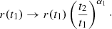
In middle panel of this figure, we also check, in the regime dominated by centrifugal force, for self-similarity in time of the spiral shape, namely that if one considers the system at two different times, t₁ and t₂, the state at t = t₂ should superpose to the state at t = t₁ rescaled as follows

$$\begin{array}{cc}\hfill {\upsilon }_{\mathrm{r}}(t_1)& \hfill \to {\upsilon }_{\mathrm{r}}(t_1){\left(\frac{t_2}{t_1}\right)}^{{\alpha }_2},\hfill \end{array}$$(47)

$$\begin{array}{cc}\hfill r(t_1)& \hfill \to r(t_1){\left(\frac{t_2}{t_1}\right)}^{{\alpha }_1}·\hfill \end{array}$$(48)

Of course, since we have two distinct self-similar regimes, this property works well only in the neighbourhood of υ_r ≃ 0 and for values of r where the gravitational force is sub-dominant compared to the centrifugal force.

Finally, the right panel of Fig. 9 shows that if gravitational potential is known, the spiral shape of the phase-space distribution function can be fully reconstructed accurately simply by knowing its intersection with the υ_r = 0 axis in the regime dominated by angular momentum (or reversely, in the regime dominated by gravitational force) by simple linear interpolation of the specific energy E along the spiral during an orbit in the following angle coordinate 𝒜,

$$\begin{array}{cc}\hfill \mathcal{A}(s,E)& \hfill \equiv 2\pi \frac{\tau (s,E)}{T(E)},\hfill \end{array}$$(49)

$$\begin{array}{cc}\hfill \tau (s,E)& \hfill ={\displaystyle {\int }_0^s\frac{\mathrm{d}r(s^{\prime })}{{\upsilon }_{\mathrm{r}}(s^{\prime })}},\hfill \end{array}$$(50)

$$\begin{array}{cc}\hfill T(E)& \hfill ={\displaystyle \oint \frac{\mathrm{d}r(s^{\prime })}{{\upsilon }_{\mathrm{r}}(s^{\prime })}},\hfill \end{array}$$(51)

where s is a curvilinear coordinate. This technique was actually used to draw the spiral of the middle panel. Of course, this result is kind of trivial from a dynamical point of view. However, it suggests that passing to action-angle space or energy-angle as performed here may represent the best way to smoothly connect both self-similar regimes and therefore to have a full analytic description of the fine grained structure of the phase-space distribution function. To do this, one needs to relate locally the angular variable Ψ intervening in the self-similar solutions to the angle given by Eq. (49), but this is left for future work.

5. Conclusion

In this article, we carried out a detailed analysis of the phase-space structure of various systems with spherical initial conditions, consisting in a power-law density profile with a Gaussian velocity dispersion. Two cases were considered: the “warm” set-up with virial ratio η ≃ 0.5 and the “cool” one with η ≃ 0.1. The choice of such initial conditions is not really new but the numerical set-up is different from what can be found in the literature. Firstly, we compared three kind of codes, a Vlasov code, a treecode, and a shell code. Secondly, we performed this comparison with unprecedented numerical resolution, namely (N_r, N_v, N_j) = (2048, 2048, 128) for the Vlasov code and 10 million particles for the N-body simulations, up to 100 million for one Gadget-2 run.

The high resolution of our simulations allowed us to study all the fine details of the phase-space distribution function and to really distinguish, for the first time, three well-known dynamical phases of the evolution of these systems, namely, (a) a violent relaxation phase to a quasi-steady state where the phase-space density can be mainly described by a smooth spiral structure winding with time, (b) a steady-state phase during which radial instabilities can destroy the spiral structure but do not affect the macroscopic properties of the system, and (c) relaxation to a non-spherical state due to radial orbit instability in the cool cases with n ≤ −1. Obviously, we did not push the simulations long enough to approach the so-called gravothermal catastrophe regime, where a core-halo structure can appear due to collisional relaxation (see, e.g. Antonov 1962; Lynden-Bell & Wood 1968; Lynden-Bell & Eggleton 1980; Makino 1996; Baumgardt et al. 2003).

While the concept of violent relaxation phase to a quasi-steady state is a well-known process studied heavily in the literature, the fact that it is expressed as a well-defined smooth spiral structure in phase space is not trivial. Subsequent radial instabilities that can appear indeed do not introduce sufficient disorder to significantly disturb the steady state initially built from the kinematic evolution of the spiral structure. Only radial orbit instability changes the properties of the system at the coarse level. But even in this case, this happens only at small radii, the outer part of the system still being given by the quasi-steady state solution obtained previously.

These results seem to diverge from what can be obtained in the pure cold case. For instance, a similar analysis was done by Henriksen et al. (1997), but for spherical initially cold systems with power-law density profiles using a shell code: in this case, Henriksen et al. (1997) found that radial instabilities are sufficiently strong to destroy the quasi-steady self-similar state obtained during the violent relaxation phase and produce a density profile close to ρ(r)∝r⁻², hence, changing the properties of the system at the macroscopic level. However, the number of shells employed by these authors was rather small and it is possible, despite the convergence tests they did, that they missed an intermediary phase where radial instability would be sufficient to destroy the spiral while preserving, as in our case, the coarse grained properties of the distribution function. We note that this question remains rather academic as radial orbit instability is expected to be prominent for such systems when allowed to deviate from spherical symmetry, although they still present some self-similar properties (Vogelsberger et al. 2011).

In a second part of our analysis, in order to at least partly understand the dynamical processes taking place during the violent relaxation phase, we examined the properties of the spiral structure of our systems in the framework of self-similar solutions. Obviously, our systems are not fully self-similar, but we showed that they follow self-similar properties in well-defined domains of phase space. Indeed, each slice of phase space of given angular momentum can be trivially decomposed into two regions, one where centrifugal force dominates, and the other one where gravitational force dominates. While the centrifugal force j²/r³ is a pure power law, this is only approximately the case for the gravitational force. Nevertheless, this approach allowed us to partly predict the properties of the spiral structure, for instance the interfold distance at zero radial velocity. Even if that is not enough by itself to be able to fully predict the steady state ab-initio, self-similarity in phase space remains an interesting path of investigation.

Acknowledgments

We thank C. Alard for providing us the main insights about the analyses performed in Sect. 4, T. Sousbie and S. Hozumi for stimulating discussions. This work was supported in part by ANR grant ANR-13-MONU-0003. We also acknowledge the support of YITP in organising the workshop “Vlasov-Poisson: towards numerical methods without particles” in Kyoto, funded by grant YITP-T-15-02, ANR grant ANR-13-MONU-0003 and by Institut Lagrange de Paris (ANR-10-LABX-63 and ANR-11-IDEX-0004-02).

References

All Tables

All Figures

	Fig. 1. Snapshots of the phase-space density for the simulations with “warm” initial conditions, η ≃ 0.5. A typical slice of f(r, υr, j) with j = 0.16 is shown in (r, υr) space for the VlaSolve simulations at t = 0, at an early time t = 15, at an intermediate time used to perform tests of self-similarity of the phase-space spiral and at the final time.
In the text

	Fig. 2. As in Fig. 1 but for the simulations with “cool” initial conditions, η ≃ 0.1 and for a slice with j = 0.06.
In the text

Fig. 3. Closer examination of the onset of instabilities in phase space for the (η, n) = (0.1, −1.5) simulations: effects of spatial and mass resolutions. For the same angular momentum slice, j = 0.06, as in lower panels of Fig. 2, the phase space density is represented in (r, υr) space. The two first lines of panels correspond to two VlaSolve simulations with respective resolutions (Nr, Nv, Nj) = (2048, 2048, 128) and (1024, 512, 512). The next two lines of panels correspond to two Gadget-2 simulations with respective numbers of particles N = 107 and N = 108 and the last line of panels gives, for N = 107, the result obtained for the shell code. For the N-body simulations, the phase-space density is sampled on grids with resolution (Nr, Nv, Nj) = (1024, 1024, 32). One can notice that the phase-space sheet is less well defined or “fuzzier” in the N-body simulations than in the Vlasov code at low radius; this is because what is actually plotted is the distribution of particles (or shells) in a relatively large interval of angular momentum j ∈ [0.056, 0.077] to have sufficient number of particles to trace the phase-space distribution function, while for the Vlasov simulation, we selected only the slice corresponding to the value of j of interest. This figure illustrates the effect of radial instabilities and their dependence on spatial resolution (for the Vlasov code) or mass resolution (for the N-body code). We note the close agreement between the shell simulation and the Gadget-2 runs with 10 million particles in the middle panels of the third and fifth lines, while they diverge in the right panels when radial orbit instability effects become prominent in Gadget-2.

In the text

Fig. 4. Radial density profile measured at various times in the VlaSolve simulations, namely initial conditions (blue dashes), intermediate time used to perform tests of self-similarity of the phase-space spiral (green), and final time (red dashes). For the final time, the results are also compared to a Gadget-2 run (thick grey), as well as the output of the shell code (thick grey dashes) for (η, n) = (0.1, −1) and (0.1, −1.5). In addition, the logarithmic slopes −4 and −2.1 (as measured in Hozumi et al. 2000) are shown respectively as a thin solid and a thin dashed line.

In the text

Fig. 5. Velocity anisotropy and deviation from sphericity. Left panel: Velocity anisotropy parameter $\alpha =2\langle {\upsilon }_{\text{r}}^2\rangle /\langle {\upsilon }_{\perp }^2\rangle$ as a function of time for the VlaSolve (solid lines) and Gadget-2 simulations we performed (dashed curves). Right panel: Evolution of the departure from spherical symmetry for the two kind of initial conditions experiencing radial orbit instability in Gadget-2, namely (η, n) = (0.1, −1.0) (blue curves) and (η, n) = (0.1, −1.5) (red curves, solid and dashed for the 10 and 100 million particles simulations, respectively). The quantity $\mathrm{sgn}(1-{\mathrm{r}}_{\mathrm{axis}}){log}_{10}|1-{\mathrm{r}}_{\mathrm{axis}}|$ indicates the deviation from unity of raxis (in log scale and with a negative sign for raxis >  1), where raxis = b/c (upper curves) or b/a (lower curves), and a ≤ b ≤ c are the principal axis lengths of the Gadget-2 particle distribution derived from the inertia tensor.

In the text

Fig. 6. Small and large radii regimes in the (η, n) = (0.5, −1) VlaSolve run at t = 40. Left panel: plots separately the magnitude of centrifugal force j2/r3 and of the gravitational force as functions of radius as well as the magnitude of the sum of both forces. Right panel: isocontours of the specific energy (white curves) superposed on the phase-space distribution function for j = 0.16. In addition, the white dashes and dot-dashes assume that only the gravitational or the centrifugal force contributes, respectively.

In the text

Fig. 7. Illustration of the method used to determine the positions of the folds and corresponding interfold distance law at small radius in a phase-space slice. Top panel: zoom performed around the axis υr = 0 in the region dominated by centrifugal force for the (η, n) = (0.5, −1.0) simulation at t = 40. The corresponding phase-space distribution function f(r, υr = 0, j = 0.16) is plotted in the lower panel. The black dots give the positions of local maxima estimated with our local quadratic fit, while the blue and red dots provide upper and lower bounds to compute the (very conservative) error bars shown on Fig. 8.

In the text

Fig. 8. Interfold distance at null radial velocity vs. self-similar predictions for a fixed value of angular momentum. The distance dr between local maxima of the function f(r, υr = 0, j) is plotted as a function of r for the VlaSolve runs with various initial conditions. The time considered corresponds to the middle column of panels in Figs. 1 and 2. The two left columns of panels correspond to the “warm” case, η = 0.5 with j = 0.16, and the two right ones to the “cool” case, η = 0.1 with j = 0.06. Then, odd column numbers (1 and 3) and even column numbers (2 and 4) correspond to the regime where centrifugal/gravitational force dominates, respectively. On each panel a red line indicates the logarithmic slope predicted by self-similarity. When the gravitational force dominates, two additional dashed curves provide a bracket of the estimated slope taking into account deviations from self-similarity, i.e. variations of the effective logarithmic slope of the gravitational force.

In the text

Fig. 9. Spiral shape vs. self-similar predictions for the VlaSolve run with (η, n) = (0.5, −1.0). Left panel: comparison, at t = 40, of the local shape of the spiral structure in the region dominated by centrifugal force to the curve given by Eq. (46) (red curve). Middle panel: test for self-similarity in time. The green spiral shape obtained at t = 30 is rescaled according to Eqs. (47) and (48) to be compared to the blue one, in the regime dominated by centrifugal force. Right panel: using only the determination of the position of the folds in the region dominated by centrifugal force, it is possible to draw the full shape of the spiral if the gravitational potential is known by interpolating the specific energy in angle coordinate defined by Eqs. (49)–(51).

In the text

References

- Aarseth, S. J., Lin, D. N. C., & Papaloizou, J. C. B. 1988, ApJ, 324, 288 [NASA ADS] [CrossRef] [Google Scholar]
- Alard, C. 2013, MNRAS, 428, 340 [NASA ADS] [CrossRef] [Google Scholar]
- Antonov, V. A. 1962, Vest. Leningrad Univ., 7, 135 [NASA ADS] [Google Scholar]
- Arad, I., & Johansson, P. H. 2005, MNRAS, 362, 252 [NASA ADS] [CrossRef] [Google Scholar]
- Arad, I., & Lynden-Bell, D. 2005, MNRAS, 361, 385 [NASA ADS] [CrossRef] [Google Scholar]
- Barnes, J., Hut, P., & Goodman, J. 1986, ApJ, 300, 112 [NASA ADS] [CrossRef] [Google Scholar]
- Barnes, E. I., Lanzel, P. A., & Williams, L. L. R. 2009, ApJ, 704, 372 [NASA ADS] [CrossRef] [Google Scholar]
- Baumgardt, H., Heggie, D. C., Hut, P., & Makino, J. 2003, MNRAS, 341, 247 [NASA ADS] [CrossRef] [Google Scholar]
- Benhaiem, D., Joyce, M., SylosLabini, F., & Worrakitpoonpon, T. 2018, MNRAS, 473, 2348 [NASA ADS] [CrossRef] [Google Scholar]
- Beraldo e Silva, L., de Siqueira Pedra, W., Sodré, L., Perico, E. L. D., & Lima, M. 2017, ApJ, 846, 125 [NASA ADS] [CrossRef] [Google Scholar]
- Bernardeau, F., Colombi, S., Gaztañaga, E., & Scoccimarro, R. 2002, Phys. Rev., 367, 1 [Google Scholar]
- Bertschinger, E. 1985, ApJS, 58, 39 [NASA ADS] [CrossRef] [Google Scholar]
- Bertschinger, E. 1998, ARA&A, 36, 599 [NASA ADS] [CrossRef] [Google Scholar]
- Binney, J. 2004, MNRAS, 350, 939 [NASA ADS] [CrossRef] [Google Scholar]
- Boily, C. M., Athanassoula, E., & Kroupa, P. 2002, MNRAS, 332, 971 [NASA ADS] [CrossRef] [Google Scholar]
- Burkert, A. 1990, MNRAS, 247, 152 [NASA ADS] [Google Scholar]
- Cannizzo, J. K., & Hollister, T. C. 1992, ApJ, 400, 58 [NASA ADS] [CrossRef] [Google Scholar]
- Carron, J., & Szapudi, I. 2013, MNRAS, 432, 3161 [NASA ADS] [CrossRef] [Google Scholar]
- Carter, B., & Henriksen, R. N. 1991, J. Math. Phys., 32, 2580 [NASA ADS] [CrossRef] [Google Scholar]
- Cheng, C. Z., & Knorr, G. 1976, J. Comput. Phys., 22, 330 [NASA ADS] [CrossRef] [Google Scholar]
- Colombi, S. 2001, New Astron., 45, 373 [CrossRef] [Google Scholar]
- Colombi, S., & Touma, J. 2008, Commun. Nonlinear Sci. Numer. Simul., 13, 46 [NASA ADS] [CrossRef] [Google Scholar]
- Colombi, S., Sousbie, T., Peirani, S., Plum, G., & Suto, Y. 2015, MNRAS, 450, 3724 [NASA ADS] [CrossRef] [Google Scholar]
- Dehnen, W., & McLaughlin, D. E. 2005, MNRAS, 363, 1057 [NASA ADS] [CrossRef] [MathSciNet] [Google Scholar]
- Dehnen, W., & Read, J. I. 2011, Eur. Phys. J. Plus, 126, 55 [CrossRef] [Google Scholar]
- Dolag, K., Borgani, S., Schindler, S., Diaferio, A., & Bykov, A. M. 2008, Space Sci. Rev., 134, 229 [NASA ADS] [CrossRef] [Google Scholar]
- Fillmore, J. A., & Goldreich, P. 1984, ApJ, 281, 1 [NASA ADS] [CrossRef] [Google Scholar]
- Fujiwara, T. 1981, PASJ, 33, 531 [NASA ADS] [Google Scholar]
- Fujiwara, T. 1983, PASJ, 35, 547 [NASA ADS] [Google Scholar]
- Gott, III, J. R., & Thuan, T. X. 1976, ApJ, 204, 649 [NASA ADS] [CrossRef] [Google Scholar]
- Hénon, M. 1964, Ann. d’Astrophys., 27, 83 [NASA ADS] [Google Scholar]
- Hénon, M. 1973, A&A, 24, 229 [Google Scholar]
- Henriksen, R. N., & Widrow, L. M. 1995, MNRAS, 276, 679 [NASA ADS] [CrossRef] [Google Scholar]
- Henriksen, R. N., & Widrow, L. M. 1997, Phys. Rev. Lett., 78, 3426 [NASA ADS] [CrossRef] [Google Scholar]
- Hjorth, J., & Williams, L. L. R. 2010, ApJ, 722, 851 [NASA ADS] [CrossRef] [Google Scholar]
- Hockney, R. W., & Eastwood, J. W. 1988, Computer Simulation Using Particles (Bristol: Hilger) [CrossRef] [Google Scholar]
- Hozumi, S., Fujiwara, T., & Kan-Ya, Y. 1996, PASJ, 48, 503 [NASA ADS] [CrossRef] [Google Scholar]
- Hozumi, S., Burkert, A., & Fujiwara, T. 2000, MNRAS, 311, 377 [NASA ADS] [CrossRef] [Google Scholar]
- Joyce, M., & Worrakitpoonpon, T. 2011, Phys. Rev. E, 84, 011139 [NASA ADS] [CrossRef] [Google Scholar]
- Joyce, M., Marcos, B., & Sylos Labini, F. 2009, MNRAS, 397, 775 [NASA ADS] [CrossRef] [Google Scholar]
- Kandrup, H. E., & Smith, Jr., H. 1991, ApJ, 374, 255 [NASA ADS] [CrossRef] [Google Scholar]
- Lynden-Bell, D. 1967, MNRAS, 136, 101 [NASA ADS] [CrossRef] [Google Scholar]
- Lynden-Bell, D., & Eggleton, P. P. 1980, MNRAS, 191, 483 [NASA ADS] [Google Scholar]
- Lynden-Bell, D., & Wood, R. 1968, MNRAS, 138, 495 [NASA ADS] [Google Scholar]
- Makino, J. 1996, ApJ, 471, 796 [NASA ADS] [CrossRef] [Google Scholar]
- Maréchal, L., & Perez, J. 2011, Transp. Theory Stat. Phys., 40, 425 [NASA ADS] [CrossRef] [Google Scholar]
- Melott, A. L. 2007, ArXiv e-prints [arXiv:0709.0745] [Google Scholar]
- Melott, A. L., Shandarin, S. F., Splinter, R. J., & Suto, Y. 1997, ApJ, 479, L79 [NASA ADS] [CrossRef] [Google Scholar]
- Merritt, D., & Aguilar, L. A. 1985, MNRAS, 217, 787 [NASA ADS] [CrossRef] [Google Scholar]
- Mohayaee, R., & Shandarin, S. F. 2006, MNRAS, 366, 1217 [NASA ADS] [CrossRef] [Google Scholar]
- Navarro, J. F., Frenk, C. S., & White, S. D. M. 1996, ApJ, 462, 563 [NASA ADS] [CrossRef] [Google Scholar]
- Navarro, J. F., Frenk, C. S., & White, S. D. M. 1997, ApJ, 490, 493 [NASA ADS] [CrossRef] [Google Scholar]
- Nishida, M. T., Yoshizawa, M., Watanabe, Y., Inagaki, S., & Kato, S. 1981, PASJ, 33, 567 [NASA ADS] [Google Scholar]
- Polyachenko, V. L., & Shukhman, I. G. 1981, Sov. Astron., 25, 533 [NASA ADS] [Google Scholar]
- Polyachenko, E. V., & Shukhman, I. G. 2015, MNRAS, 451, 601 [NASA ADS] [CrossRef] [Google Scholar]
- Pontzen, A., & Governato, F. 2013, MNRAS, 430, 121 [NASA ADS] [CrossRef] [Google Scholar]
- Romero, M., & Ascasibar, Y. 2018, MNRAS, 479, 4225 [NASA ADS] [CrossRef] [Google Scholar]
- Sikivie, P., Tkachev, I. I., & Wang, Y. 1997, Phys. Rev. D, 56, 1863 [NASA ADS] [CrossRef] [Google Scholar]
- Sousbie, T., & Colombi, S. 2016, J. Comput. Phys., 321, 644 [NASA ADS] [CrossRef] [Google Scholar]
- Springel, V. 2005, MNRAS, 364, 1105 [NASA ADS] [CrossRef] [Google Scholar]
- Taylor, J. E., & Navarro, J. F. 2001, ApJ, 563, 483 [NASA ADS] [CrossRef] [Google Scholar]
- Tremaine, S., Hénon, M., & Lynden-Bell, D. 1986, MNRAS, 219, 285 [NASA ADS] [CrossRef] [Google Scholar]
- Vogelsberger, M., Mohayaee, R., & White, S. D. M. 2001, MNRAS, 414, 3044 [NASA ADS] [CrossRef] [Google Scholar]
- Watanabe, Y., Inagaki, S., Nishida, M. T., Tanaka, Y. D., & Kato, S. 1981, PASJ, 33, 541 [NASA ADS] [Google Scholar]
- Yamaguchi, Y. Y. 2008, Phys. Rev. E, 78, 041114 [NASA ADS] [CrossRef] [Google Scholar]
- Yamashiro, T., Gouda, N., & Sakagami, M. 1992, Prog. Theor. Phys., 88, 269 [NASA ADS] [CrossRef] [Google Scholar]