| Issue |
A&A
Volume 621, January 2019
|
|
|---|---|---|
| Article Number | A126 | |
| Number of page(s) | 17 | |
| Section | Catalogs and data | |
| DOI | https://doi.org/10.1051/0004-6361/201833316 | |
| Published online | 18 January 2019 | |
CARMENES input catalogue of M dwarfs
IV. New rotation periods from photometric time series⋆
1
Departamento de Astrofísica y Ciencias de la Atmósfera, Facultad de Ciencias Físicas, Universidad Complutense de Madrid, 280140 Madrid, Spain
e-mail: This email address is being protected from spambots. You need JavaScript enabled to view it.
2
Departamento de Explotación y Prospección de Minas, Escuela de Minas, Energía y Materiales, Universidad de Oviedo, 33003 Oviedo, Asturias, Spain
3
Observatorio Astronómico Carda, MPC Z76 Villaviciosa, Asturias, Spain
4
Centro de Astrobiología (CSIC-INTA), Campus ESAC, Camino Bajo del Castillo s/n, 28692 Villanueva de la Cañada, Madrid, Spain
5
Institut für Astrophysik, Georg-August-Universität Göttingen, Friedrich-Hund-Platz 1, 37077 Göttingen, Germany
6
AstroLAB IRIS, Provinciaal Domein “De Palingbeek”, Verbrandemolenstraat 5, 8902 Zillebeke, Ieper, Belgium
7
Observatorio Astronómico Naves, (MPC 213) Cabrils, Barcelona, Spain
8
Institut de Ciències de l’Espai (CSIC-IEEC), Campus UAB, c/ de Can Magrans s/n, 08193 Bellaterra, Barcelona, Spain
9
Institut d’Estudis Espacials de Catalunya (IEEC), 08034 Barcelona, Spain
10
Vereniging Voor Sterrenkunde, Brugge, Belgium & Centre for Mathematical Plasma Astrophysics, Katholieke Universiteit Leuven, Celestijnenlaan 200B, bus 2400, 3001 Leuven, Belgium
11
Instituto de Astrofísica de Andalucía (CSIC), Glorieta de la Astronomía s/n, 18008 Granada, Spain
12
Instituto de Astrofísica de Canarias, c/ Vía Láctea s/n, 38205 La Laguna, Tenerife, Spain
13
Departamento de Astrofísica, Universidad de La Laguna, 38206 La Laguna, Tenerife, Spain
14
Max-Planck-Institut für Astronomie, Königstuhl 17, 69117 Heidelberg, Germany
15
Landessternwarte, Zentrum für Astronomie der Universität Heidelberg, Königstuhl 12, 69117 Heidelberg, Germany
16
School of Geosciences, Raymond and Beverly Sackler Faculty of Exact Sciences, Tel Aviv University, Tel Aviv 6997801, Israel
Received:
27
April
2018
Accepted:
4
September
2018
Abstract
Aims. The main goal of this work is to measure rotation periods of the M-type dwarf stars being observed by the CARMENES exoplanet survey to help distinguish radial-velocity signals produced by magnetic activity from those produced by exoplanets. Rotation periods are also fundamental for a detailed study of the relation between activity and rotation in late-type stars.
Methods. We look for significant periodic signals in 622 photometric time series of 337 bright, nearby M dwarfs obtained by long-time baseline, automated surveys (MEarth, ASAS, SuperWASP, NSVS, Catalina, ASAS-SN, K2, and HATNet) and for 20 stars which we obtained with four 0.2–0.8 m telescopes at high geographical latitudes.
Results. We present 142 rotation periods (73 new) from 0.12 d to 133 d and ten long-term activity cycles (six new) from 3.0 a to 11.5 a. We compare our determinations with those in the existing literature; we investigate the distribution of Prot in the CARMENES input catalogue, the amplitude of photometric variability, and their relation to v sini and pEW(Hα); and we identify three very active stars with new rotation periods between 0.34 d and 23.6 d.
Key words: stars: activity / stars: late-type / stars: rotation / techniques: photometric
Tables A.1 and A.2, and tables of the photometric measurements are only available at the CDS via anonymous ftp to cdsarc.u-strasbg.fr (130.79.128.5) or via http://cdsarc.u-strasbg.fr/viz-bin/qcat?J/A+A/621/A126
© ESO 2019
1. Introduction
In current exoplanet search programmes, knowledge of the stellar rotation periods is essential in order to distinguish radial-velocity signals induced by real planets or by the rotation of the star itself (Saar & Donahue 1997; Queloz et al. 2001; Boisse et al. 2011). This is even more important when the goal is to detect weak signals induced by Earth-like exoplanets around low-mass stars (Scalo et al. 2007; Léger et al. 2009; Dumusque et al. 2012; Anglada-Escudé et al. 2016). For this purpose, star spots on the photosphere of stars can help us because they induce a photometric modulation from which we can infer not only the rotation period of the stars (Kron 1947; Bouvier et al. 1993; Messina & Guinan 2002; Strassmeier 2009), but also long-term activity cycles (Baliunas & Vaughan 1985; Berdyugina & Järvinen 2005).
M dwarfs are strongly affected by star spots because of the presence of large active regions on their surfaces, which are due to the depth of the convective layers (Delfosse et al. 1998; Mullan & MacDonald 2001; Browning 2008; Reiners & Basri 2008; Barnes et al. 2011) As a result, these late-type stars are the most likely to present this kind of modulation in photometric series (Irwin et al. 2011; Kiraga 2012; West et al. 2015; Suárez Mascareño et al. 2016). The low masses and small radii of M dwarfs also make them ideal targets for surveys aimed at detecting small, low-mass, potentially habitable Earth-like planets (Joshi et al. 1997; Segura et al. 2005; Tarter et al. 2007; Reiners et al. 2010; France et al. 2013). Therefore, the inclusion of M-dwarf targets in exoplanet surveys has increased steadily from the first dedicated radial-velocity searches (Butler et al. 2004; Bonfils et al. 2005; Johnson et al. 2007), through transit searches from the ground and space (Berta et al. 2013; Kopparapu et al. 2013; Crossfield et al. 2015; Dressing & Charbonneau 2015; Gillon et al. 2016, 2017; Dittmann et al. 2017), to up-to-date searches with specially designed instruments and space missions such as CARMENES (Quirrenbach et al. 2014), HPF (Mahadevan et al. 2014), IRD (Tamura et al. 2012), SPIRou (Artigau et al. 2014), TESS (Ricker et al. 2015), or GIARPS (Claudi et al. 2016). As a result, there is a growing number of projects aimed at photometrically following up large samples of M dwarfs in the solar neighbourhood with the goals of determining their rotation periods and discriminating between signals induced by rotation from those induced by the presence of planets (Irwin et al. 2011; Suárez Mascareño et al. 2015; Newton et al. 2016). Some of the targeted M dwarfs have known exoplanets, or are suspected to harbour them, while others are just being monitored by radial-velocity surveys with high-resolution spectrographs. Some exoplanets may transit their stars, although transiting exoplanets around bright M dwarfs are rare (Gillon et al. 2007; Charbonneau et al. 2009).
This work is part of the CARMENES project1. It is also the fourth item in the series of papers devoted to the scientific preparation of the target sample being monitored during CARMENES guaranteed time observations (see also Alonso-Floriano et al. 2015a; Cortés-Contreras et al. 2017; Jeffers et al. 2018). Here we present the results of analysing long-term, wide-band photometry of 337 M dwarfs currently being monitored by CARMENES (Reiners et al. 2018b). For many of them we had not been able to find rotation periods in the existing literature (see below).
To determine the rotation periods of our M dwarfs, we make extensive use of public time series of wide-area photometric surveys and databases such as the All-Sky Automated Survey (ASAS; Pojmański 1997), Northern Sky Variability Survey (NSVS; Woźniak et al. 2004), Wide Angle Search for Planets (SuperWASP; Pollacco et al. 2006), Catalina Real-Time Transient Survey (Catalina; Drake et al. 2009), and The MEarth Project (MEarth; Charbonneau et al. 2009; Irwin et al. 2011). Since the amplitude of the modulations induced by star spots, in the range of millimagnitudes, is also within reach of current amateur facilities (Herrero et al. 2011; Baluev et al. 2015), we also collaborate with amateur astronomers to obtain data for stars that have never been studied by systematic surveys or that need a greater number of observations.
After collecting and cleaning the time series, we look for significant peaks in power spectra, determine probable rotation periods and long activity cycles, compare them with previous determinations and activity indicators when available, and make all our results available to the whole community in order to facilitate the disentanglement of planetary and activity signals in current and forthcoming radial-velocity surveys of M dwarfs.
2. Data
2.1. Sample of observed M dwarfs
During guaranteed time observations (GTOs), the double-channel CARMENES spectrograph has so far observed a sample of 336 bright, nearby M dwarfs with the goal of detecting low-mass planets in their habitable zone with the radial-velocity method (Quirrenbach et al. 2015; Reiners et al. 2018b): 324 have been presented by Reiners et al. (2018b), 3 did not have enough CARMENES observations at the time the spectral templates were being prepared for the study, and 9 are new spectroscopic binaries (Baroch et al. 2018). Here we investigate the photometric variability of these 336 M dwarfs and of G 34–23 AB (J01221+221AB), which Cortés-Contreras et al. (2017) found to be a close physical binary just before the GTOs started. This results in a final sample size of 337 stars.
As part of the full characterisation of the GTO sample, for each target we have collected all relevant information: astrometry, photometry, spectroscopy, multiplicity, stellar parameters, and activity, including X-ray count rates, fluxes, and hardness ratios, Hα pseudo-equivalent widths, reported flaring activity, rotational velocities v sini, and rotational periods Prot (Caballero et al. 2016). In particular, for 69 stars of the CARMENES GTO sample we had already collected rotation periods from the existing literature (e.g. Kiraga & Stepien 2007; Norton et al. 2007; Hartman et al. 2011; Irwin et al. 2011; Kiraga 2012; Suárez Mascareño et al. 2015; West et al. 2015; Newton et al. 2016, see below).
Of the 337 investigated stars, we were unable to collect or measure any photometric data useful for variability studies for only 3. In these three cases, the M dwarfs are physical companions at relatively small angular separations of bright primaries (J09144+526 = HD 79211, J11110+304 = HD 97101 B, and J14251+518 = θ Boo B). For the other 334 M dwarfs, we looked for peaks in the periodograms of two large families of light curves that we obtained (i) from wide-area photometric surveys and public databases, and (ii) with 20–80 cm telescopes at amateur and semi-professional observatories. A more detailed photometric survey of particular GTO targets is being carried out within the CARMENES consortium with more powerful telescopes, such as the Las Cumbres Observatory Global Telescope Network (Brown et al. 2013) and the Instituto de Astrofísica de Andalucía 1.5 m and 0.9 m telescopes at the Observatorio de Sierra Nevada. Results of this photometric monitoring extension will be published elsewhere.
In the first four columns of Table A.1 we give the Carmencita identifier (Caballero et al. 2016), discovery name, and 2MASS (Skrutskie et al. 2006) equatorial coordinates of the 337 M dwarfs investigated in this work.
2.2. Photometric monitoring surveys
We searched for photometric data of our target stars, available through either VizieR (Ochsenbein et al. 2000) or, more often, the respective public web pages of the four main wide-area surveys listed below and summarised in the top part of Table 1.
MEarth: The MEarth Project2 (Nutzman & Charbonneau 2008; Irwin et al. 2011). This consists of two robotically-controlled 0.4 m telescope arrays, MEarth-North at the the Fred Lawrence Whipple Observatory on Mount Hopkins, Arizona, and MEarth-South telescope at the Cerro Tololo Inter-American Observatory, Coquimbo. The project monitors the brightness of about 2000 nearby M dwarfs with the goal of finding transiting planets (Berta et al. 2013; Dittmann et al. 2017), but it has also successfully measured rotation periods of M dwarfs (Irwin et al. 2009, 2011; Newton et al. 2016). On every clear night and for about six months, each star is observed with a cadence of 20 min. In general we used data from three observing batches (2008–2010, 2010–2011, and 2011–2015) from the MEarth-North array (δ = +20 to +60) provided by the fifth MEarth data release DR5, but we also used a few DR6 light curves (2011–2016).
ASAS: All-Sky Automated Survey3 (Pojmański 2002). This is a Polish project devoted to constant photometric monitoring of the whole available sky (approximately 20 million stars brighter than V ∼ 14 mag). It consists of two observing stations in Las Cumbres Observatory, Chile (ASAS-3 from 1997 to 2010, ASAS-4 since 2010), and Haleakalā Observatory, Hawai’i (ASAS-3N since 2006). Both are equipped with two wide-field instruments observing simultaneously in the V and I bands, and a set of smaller narrow-field telescopes and wide-field cameras. We used only the V-band ASAS-3 data for stars with δ < +28 deg observed between 1997 and 2006, which are available through the ASAS All Star Catalogue. In particular, we retrieved all light curves within a search radius of 15 arcsec, discarded all data points with C or D quality flags, and computed an average magnitude per epoch of the five ASAS-3 apertures weighted by each aperture magnitude error.
SuperWASP: Super-Wide Angle Search for Planets4 (Pollacco et al. 2006). The UK-Spanish WASP consortium runs two identical robotic telescopes of eight lenses each, SuperWASP-North at the Observarorio del Roque de los Muchachos, La Palma, and SuperWASP-South at the South African Astronomical Observatory, Sutherland. WASP has discovered over a hundred exoplanets through transit photometry (Collier Cameron et al. 2007; Barros et al. 2011). For our work, we downloaded light curves of the first SuperWASP public data release (DR1 – Butters et al. 2010) from the Czech site5. The SuperWASP DR1 contains light curves for about 18 million sources in both hemispheres. Although the two robotic telescopes are still operational, DR1 only provided data collected from 2004 to 2008. The average number of data points per light curve is approximately 6700.
NSVS: Northern Sky Variability Survey6 (Woźniak et al. 2004). This was located at Los Álamos National Laboratory, New Mexico. The NSVS catalogue contains data from approximately 14 million objects in the range V = 8–15.5 mag with a typical baseline of one year from April 1999 to March 2000, and 100–500 measurements for each source. In a median field, bright unsaturated stars have photometric scatter of about 20 mmag. It covered the entire northern hemisphere, and part of the southern hemisphere down to δ = –28 deg.
In addition to these four main catalogues, which accounted for a total of 533 light curves (86%), we complemented our dataset with light curves compiled from the Catalina Surveys CSDR27 (Catalina; Drake et al. 2009, 2014), K2 (Howell et al. 2014), the All-Sky Automated Survey for Supernovae8 (ASAS-SN; Kochanek et al. 2017), and the Hungarian-made Automated Telescope Network9 (HATNet; Bakos et al. 2004; Bakos 2018). None of our targets was in the catalogues of the CoRoT (Auvergne et al. 2009), Kepler (Borucki et al. 2010), or the Transatlantic Exoplanet Survey (TrES; Alonso et al. 2007) surveys. Finally, we did not use other wide surveys, such as Lincoln Near-Earth Asteroid Research (LINEAR; Stokes et al. 2000); XO (McCullough et al. 2005); Kilodegree Extremely Little Telescope (KELT; Pepper et al. 2007), which will soon have an extensive data release (Pepper, priv. comm.); HATSouth (Bakos et al. 2013); or the Asteroid Terrestrial-impact Last Alert System (ATLAS; Heinze et al. 2018), with the first data release published after collecting all light curves included in this work. All the public surveys used, amounting 602 light curves, are summarised in Table 1.
Number of investigated light curves and basic parameters of used public surveys and observatories.
2.3. Our observations
For 20 GTO M dwarfs without data in public surveys or published periods, or with unreliable or suspect periods in the existing literature (e.g. short Prot, lit but low v sini and faint Hα emission, or vice versa), we made our own observations in collaboration with amateur and semi-professional astronomical observatories in Spain and Belgium: Carda10 (MPC Z76) in Asturias, Montcabrer11 (MPC 213) and Montsec12 in Barcelona (MPC C65), and AstroLAB IRIS13 near Ypres. Most of our targets had northern declinations, which suitably fit the geographical latitudes of our observatories (between +41.5 deg and +50.8 deg).
The cadence of observations for each target was either continuous every night or just one observation per night during a long run, depending on rule-of-thumb estimations of their rotation periods based on literature values of rotational velocity and Hα emission. Exposure times varied widely, from a few seconds to several minutes. We took special care to select enough reference stars with stable light curves and relatively red J − Ks colours within the respective fields of view (f.o.v.; variable from 12.3 × 12.3 arcmin2 to 43 × 43 arcmin2).
For the image reduction and light-curve generation, we used standard calibration procedures (bias and flat-field correction) and widely distributed software such as MaxIm14, AstroImageJ15 (Collins et al. 2017), FotoDif16, and LesvePhotometry17 with parameters appropriate for each observatory, atmospheric condition, and star brightness (see again Table 1).
3. Analysis
We searched for significant signals in the periodograms of the 622 light curves compiled or obtained by us as described in Sect. 2. Prior to this, we cleaned our light curves by discarding outlying data points caused by the combination of target faintness and sub-optimal weather. Some of our M dwarfs could also undergo flaring activity (most flares in our light curves are difficult to identify because of the typical low cadence). We used the same cleaning procedure as Suárez Mascareño et al. (2015, 2016), rejecting iteratively all data points that deviated more than 2.5σ from the mean magnitude (which might eventually bias the amplitude of the variations).
The last six columns of Table A.1 show the corresponding survey, number of data points Nobs before and after the cleaning, time interval length Δt between first and last visit, mean m̅ and standard deviation σm of the individual magnitudes, and mean error  . See Sect. 4.4 for a discussion on the variation of σm as a function of m̅, and the possibility of finding aperiodic or irregular variable stars in our data.
Next, we used the Lomb–Scargle (LS) periodogram (Scargle 1982) with the peranso analysis software (Paunzen & Vanmunster 2016), which implements multiple light-curve and period analysis functions. We evaluated the significance of the signals found in the periodograms with the Cumming (2004) modification of the Horne & Baliunas (1986) formula. In this way, the false alarm probability (FAP) becomes
![Mathematical equation: $$ \begin{aligned} \mathrm{FAP} = 1 - [1 - p(z>z_0)]^M, \end{aligned} $$](/articles/aa/full_html/2019/01/aa33316-18/aa33316-18-eq2.gif) (1)
(1)
with p(z > z0) being the probability that z, the target spectral density, is greater than z0, the measured spectral density; and M the number of independent frequencies. In our case, p(z > z0)=e−z0, where z0 is the peak of the hypothetical signal; M = ΔtΔf, where Δt is the time baseline, Δf = f2 − f1; and f2 and f1 are the maximum and minimum search frequencies, respectively. The peranso software also measures amplitudes of light curves.
We searched for significant frequencies with FAP < 2% and within the standard frequency interval. On the one hand, we set the highest frequency at the Nyquist frequency to about half of the minimum time interval between consecutive visits (from f ∼ 100 d−1 for some of our intensive campaigns to f ∼ 1 d−1 for most of the public-survey light curves). On the other hand, we set the lowest frequency at half the length of the monitoring (typically f ∼ 0.005 d−1). Only in the case of ASAS, the public survey with the longest time baseline (up to ten years), did we search for low frequencies down to 0.0005 d−1. For stars with significant signals shorter than 2 d we used a significant frequency oversampling (∼10×). When a periodogram displayed several significant peaks, we paid special attention to identifying aliases and picked up the strongest signal with astrophysical meaning (e.g. with Prot consistent with existing additional information on the star, especially its rotational velocity, v sini; see Sect. 4.3). Figures B.1–B.9 illustrate our analysis with one representative example of a raw stellar light curve and corresponding LS periodogram and phase-folded light curve for each dataset with identified period.
There is a justified concern in the literature about the use of the LS periodogram for period determination (e.g. McQuillan et al. 2013). As a result, for the light curves of stars classified as new spectroscopic binaries by Baroch et al. (2018), with K2 data, or with periods shorter than 1 d, or different by more than 10% from those in the literature (see Sect. 4.1) we also applied the generalised LS periodogram method (GLS; Zechmeister & Kürster 2009).
For the spectroscopic binaries and K2 stars, we additionally applied the Gaussian process regression (GP; Rasmussen & Williams 2005) with the celerite package (Foreman-Mackey et al. 2017). To build a celerity model for our case, we defined a covariance/kernel for the GP model, which consisted of a stochastically-driven damped oscillator and a jitter term (Angus et al. 2018). We then wrapped the kernel defined in this way in the GP and computed the likelihood. In all investigated cases except two, the GLS and GP periods were identical within their uncertainties to the LS periods computed with peranso. The only two significant differences were J18356+329, for which GLS did not recover Prot = 0.118 d, the shortest period in our sample and identical to that reported by Hallinan et al. (2008), and J16254+543, for which GLS found Prot = 76.8 d, a value similar to that in the literature (Suárez Mascareño et al. 2015), but for which the LS algorithm found 100 ± 5 d.
In Table A.2 we show the periods, amplitudes, FAPs, and corresponding surveys of 142 M dwarfs. When available, we show the GLS periods. We tabulate the uncertainty in Prot from the full width at half maximum of the corresponding peak in the periodogram (Schwarzenberg-Czerny 1991). For GLS periods, we tabulate formal uncertainties, which are significantly smaller than the real ones.
When several datasets are available, and even though the periodogram peaks are detected in both, we list the Prot of the dataset with the lowest FAP. For the sake of completeness, Table A.2 includes five stars with FAP = 2–10% for which we recover periods similar to those previously published (Testa et al. 2004; Suárez Mascareño et al. 2015, 2016), but which did not pass our initial FAP criterion. One such period is for J11477+008 = FI Vir, for which Suárez Mascareño et al. (2016) reported a rotation period of 165 d consistent with ours. Its K2 light curve, which spans only 80 d, shows a clear modulation that matches such a long period, the longest one reported by us. Something similar occurs with J13458–179 = LP 798–034, whose K2 light curve shows a 20 mmag peak-to-peak modulation of about three months. We did not find any periods in the existing literature or our ASAS data for this star, which is not listed in Table A.2.
We also looked for long-period cycles in ASAS light curves of stars with identified Prot and time baseline Δt ≈ 9 a. Ten stars have significant signals at Pcycle ≥ 3.0 a, and are listed in Table 2. Two of these (J06105–218 and J15218+209) have cycle periods longer than half Δt, and one has a cycle period even longer than the full Δt, but its modulation is very clear (see Fig. 1). Curiously, the star with the longest rotation period and highest FAP, J11477+008, also displays a long-term activity cycle. This flaring M4 dwarf is also the star with the smallest ratio Pcycle/Prot ∼ 10.
Cycle periods obtained for stars in our sample.
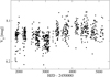 |
Fig. 1. ASAS V-band photometric data for the M0.5 V star J06105-218 = HD 42581A. It may display an activity cycle modulation with Pcycle ∼ 8.3 a superimposed to a rotation period Prot = 27.3 d (the modulation in the light curve of J15218+209 is similar). |
Of the ten values of Pcycle shown in Table 2, six are new, three are identical within their uncertainties to previous determinations by Suárez Mascareño et al. (2016), and one is revised from 9.3 a to about 3.3 a. There are two additional stars, not listed in Table 2, with significant signals (FAP < 2%) at 2–3 a, but without identified or reported rotation periods (J06371+175 and J22559+178). It may be that they truly display a long-term modulation overlaid on a low-amplitude rotation period not detected yet, as they could be pole-on.
4. Results and discussion
4.1. Rotation periods
Of the 142 stars with periods in Table A.2, 69 (49%) had rotation periods previously reported in the existing literature and tabulated in Carmencita (Caballero et al. 2016); see Table A.2 for full references. Therefore, we present 73 new photometric periods of M dwarfs in this study. This number is comparable to the number of new rotation periods of M dwarfs reported by Norton et al. (2007), Irwin et al. (2011), and Suárez Mascareño et al. (2016), but is far lower than other more comprehensive searches by Hartman et al. (2011), Kiraga (2012), and Newton et al. (2017). However, there is a fundamental difference in the samples; ours exclusively contains bright, nearby M dwarfs that are targets of dedicated exoplanet surveys. In particular, the mean J-band magnitude and heliocentric distance of our CARMENES GTO sample are only 7.7 mag and 11.6 pc (cf. Caballero et al. 2016), much brighter and closer than any M dwarf sample photometrically investigated previously.
We were not able to recover the rotation periods of 14 stars reported by Kiraga & Stepien (2007), Kiraga (2012), Suárez Mascareño et al. (2015), and Newton et al. (2016), and listed in Table 3. In most of these cases, unrecovered published Prot, lit values were long, of low significance, and came from low-cadence, relatively noisy, ASAS data.
Stars with published rotation periods not recovered in this work.
In Fig. 2 we compare the rotation periods that we found and those reported in the existing literature for the 69 stars in common. Except for four discordant stars, the agreement is excellent, with maximum deviations rarely exceeding 10%, and with virtually all values identical within their uncertainties. There are four outliers with deviations between Prot, lit and Prot, this work larger than 20%:
J00051+457 = GJ 2. A rotation period of 21.2 d was previously measured by Suárez Mascareño et al. (2015) from a series of high-resolution spectroscopy of activity indicators, while we measure 15.37 d on an ASAS light curve;
J16570–043 = LP 686–027. This is an active, “RV-loud star” (pEW(Hα) = –4.2 ± 0.1 Å and v sini ≈ 10.1 km s−1 (Jeffers et al. 2018; Reiners et al. 2018b; Tal-Or et al. 2018). Our analysis of the ASAS data reproduced the 1.21 d period of Kiraga (2012), but with an FAP ≫ 5%. However, our analysis of NSVS data, with ∼4 more epochs and a baseline ∼9 times longer than ASAS, resulted in a shorter Prot ∼ 0.55 d with a lower FAP = 1.4%;
J18363+136 = Ross 149. We found two significant signals in our ASAS data of roughly the same power at 1.02 d and 50.2 d, which are aliases of one another. The first period is identical to Prot, lit = 1.017 d discovered by Newton et al. (2016) in MEarth data. However, we tabulate the 50.2 d period based on the very slow rotation velocity of the star (v sini < 2 km s−1; Reiners et al. 2018b);
J20260+585 = Wolf 1069. Newton et al. (2016) reported a possible or uncertain period of 142.09 d. With MEarth data, we found instead a signal at 59.0 d. However, neither of the two signals is visible in the SuperWASP dataset.
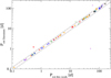 |
Fig. 2. Periods from the literature Prot, lit as a function of our period, Prot, this work, for stars with previously published rotation periods. Dashed lines show 10% and 20% deviations from the 1:1 relation. Different symbols and colours stand for the literature source: blue crosses: Norton et al. (2007); green squares: Hartman et al. (2011); blue circles: Irwin et al. (2011); red diamonds: Kiraga (2012); brown up-triangles: Kiraga & Stepien (2007); black left-triangles: Suárez Mascareño et al. (2016); violet A’s: Newton et al. (2016); green S’s: Suárez Mascareño et al. (2018); orange asterisks: Greimel & Robb (1998), Fekel & Henry (2000), Testa et al. (2004), Rivera et al. (2005), Hallinan et al. (2008), Kiraga & Stȩpień (2013), Suárez Mascareño et al. (2015), West et al. (2015), David et al. (2016), Cloutier et al. (2017), Vida et al. (2017), and Lothringer et al. (2018). |
4.2. Period distribution
Using MEarth data, Newton et al. (2016) reported that the distribution of M-dwarf rotation periods displays a lack of stars with intermediate rotation periods around 30 d. This lack at intermediate periods could be understood as a bimodal Prot distribution, with peaks at 0.5–2 d and 50–100 d, and a valley in between. While there is a significant overabundance of periods larger than 30 d in our sample, as illustrated in Fig. 3, the distribution of periods shorter than 30 d (and longer than 0.5 d) is flat within Poissonian statistics. Therefore, we see only one wide peak in the period distribution at Prot = 20–120 d or, conversely, a lack of stars with intermediate and short rotation periods Prot = 0.6–20 d. However, rather than contradicting the results presented by Newton et al. (2016), we attribute the lack of short periods to the different temporal sampling of the surveys used (see below). The authors also stated that the rotators with the highest quality grade were biased towards such short periods, while the sparse temporal sampling of most surveys used here (excluding SuperWASP and MEarth) prevented us from detecting periods of a few days. If the available periods for the ∼2200 Carmencita stars are taken into account (cf. Fig. 3), the peak at Prot = 20–120 d becomes much less apparent, and the period distribution is rather flat from 0.6 d to 8 d, approximately. There might be a dip at Prot = 8–20 d.
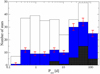 |
Fig. 3. Distribution of rotation periods in our work (shaded, with Poissonian uncertainties) and in Carmencita (white). Rotation periods found with ASAS are shaded darker. The size of the bins follows the definitions given by Freedman & Diaconis (1981). Compare with Fig. 3 in Newton et al. (2016). |
Regarding survey sampling, we analysed the distribution of time elapsed between consecutive exposures of our light curves. The SuperWASP distribution has two peaks, one very narrow at slightly less than one minute (the CCD read-out time) and another wider peak, centred at 10–20 min, a bit more optimistic than the 40 min stated by Pollacco et al. (2006). The NSVS distribution also has two peaks, one at around 1 min and the other at 1 d, much wider and sparser than SuperWASP and with a baseline of only one year (Woźniak et al. 2004). Together with SuperWASP, the MEarth dataset is, with a field cadence of between 15 and 40 min (∼20 min according to Irwin et al. 2011) and “sequentially for the entire time [that] they are above airmass 2”, the most appropriate one for sampling the Prot = 0.6–20 d interval. The ASAS sampling is much poorer than the other three main surveys, with a peak of the distribution centred at around one week. The nominal sampling value of 2 d (Pojmański 2002) is attained only for some bright stars and during a fraction of the observing time. However, the sampling strategy and the very long duration of the ASAS survey, of several years, makes it excellent for searching for periods longer than 20 d.
This partly explains the apparent lack of rotation periods in the range between 0.6 and 20 d of GTO stars with respect to Carmencita stars in Fig. 3. Our GTO stars are brighter than the rest of the Carmencita stars (Alonso-Floriano et al. 2015a) so the observed lack of shorter periods in our sample is probably caused by the inclusion of bright ASAS targets, combined with the observational cadence of ASAS, which is optimised towards detecting long periods. We thus have a combination of a Malmquist bias and a sampling effect.
A larger (volume- or magnitude-limited) sample of M dwarfs with a homogeneous, denser, longer monitoring could be needed to settle the question if there is a real lack of rotation periods between 0.6 d or 8 d and 20 d at low stellar masses. We may have to wait for the 8.4 m Large Synoptic Survey Telescope, which will monitor the entire available sky every three nights on average.
4.3. Activity
4.3.1. RV-loud stars
A comprehensive study linking rotational velocity, Hα emission, and rotation periods of M dwarfs was already presented by Jeffers et al. (2018) in a previous publication of this series. Using different tracers of magnetic activity, it can be seen that the rotational velocity increases with M-dwarf activity until saturation in rapid rotators (Stauffer et al. 1984; Hawley et al. 1996; Delfosse et al. 1998; Kiraga & Stepien 2007; Mohanty & Basri 2003; Reiners et al. 2009; Browning et al. 2010; Newton et al. 2017, and references therein).
As a complement to these studies, we present the following brief discussion on the rotation periods of the most active stars in our sample, most of which were tabulated by Tal-Or et al. (2018). They presented a list of 31 RV-loud stars: CARMENES GTO M-dwarf targets that displayed large-amplitude radial-velocity variations due to activity. Most of these stars, close to activity saturation, were also part of the investigation on wing asymmetries of Hα, Na I D, and He I lines in CARMENES spectra by Fuhrmeister et al. (2018). We found rotation periods from photometric time series for all of them except for nine stars18, J12156+526 = StKM 2–809, J14173+454 = RX J1417.3+4525, J15499+796 = LP022–420, J16555–083 = vB 8, J18189+661 = LP 071–165, J19255+096 = LSPM J1925+0938, and J20093–012 = 2MASS J20091824–0113377, which are either extremely active (e.g. Barta 161 12, LP 022–420), too faint and late for the surveys used (e.g. vB 8, 2MASS J20091824–0113377), or both (e.g. LSPM J1925+0938). The most active of these nine stars without an identified period could actually be variable, but irregular (see below).
As expected from their typically large v sini values, most of the other 22 RV-loud stars have short or very short rotation periods: 20 stars have Prot < 10 d, and 11 have Prot < 1 d. The list of RV-loud stars with identified periods contains some very well-known variable stars, such as V388 Cas, V2689 Ori, YZ CMi, DX Cnc, GL Vir, OT Ser, V1216 Sgr, V374 Peg, EV Lac, and GT Peg. However, there are three such RV-loud stars for which there was no published value of rotation period. Of these, two have identified periods shorter than one day: J02088+494 = G 173–039 (Prot = 0.748 d) and J04472+206 = RX J0447.2+2038 (Prot = 0.342 d). They both have high rotational velocities of v sini ≈ 24 − 48 km s−1 (Reiners et al. 2018a; Tal-Or et al. 2018). The third star without a previously reported rotation period is J19169+051S = V1298 Aql (vB 10, Prot = 23.6 d), which has a slow rotational velocity of only 2.7 km s−1, but it does have an M8.0 V spectral type (Alonso-Floriano et al. 2015a; Kaminski et al. 2018) and has long been known to display variability of up to 0.2 mag peak-to-peak in V band (Herbig 1956; Liebert et al. 1978).
The 31 RV-loud stars in Tal-Or et al. (2018) are not the only CARMENES GTO M-dwarf targets that display large-amplitude radial-velocity variations due to activity, as all stars with ten or fewer observations during the first 20 months of operation were discarded from the study. In total, 46 stars in our sample have rotation periods shorter than 10 d, and 19 shorter than 1 d. Of the latter, only seven were not tabulated as RV-loud stars by Tal-Or et al. (2018): four M4.0–5.5 dwarfs with previously reported rotation period and v sini > 16 km s−1, the strong X-ray emitter RBS 365 (J02519+224, M4.0 V, v sini = 27.4 ± 0.6 km s−1), the β Pictoris moving group candidate 1RXS J050156.7+010845 (J05019+011, M4.0 V, v sini = 6.1 ± 0.9 km s−1; see Alonso-Floriano et al. 2015b, and references therein), and the unconfirmed close astrometric binary G 34–23 AB (J01221+221 AB; not in the GTO sample, see Sect. 2). Because of the magnitude difference between the two components in the pair (ΔI = 0.86 ± 0.12 mag according to Cortés-Contreras et al. 2017) the most likely variable is the primary, G 34–23 A. New analyses of RV scatter and activity of CARMENES GTO stars, including the other six single stars just described and the three RV-loud stars with new periods described above, most of them with Prot < 1 d, are ongoing and will be presented elsewhere.
4.3.2. Linking Prot, vsini, Hα, and A
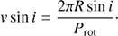
We go deeper into the Prot − v sini discussion with the top panel in Fig. 4. To build this plot we took 305 rotation periods and rotation velocities from the existing literature and compiled in the Carmencita catalogue (see references in Sect. 2.1). As expected and widely discussed by West et al. (2015) and Jeffers et al. (2018), among others, the shorter the rotation period Prot of an M dwarf, the higher the rotation velocity v sini. The vertical width is due to the indetermination in inclination angle i and the spread in spectral types, and thus stellar radii R according to the formula
 (2)
(2)
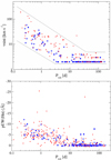 |
Fig. 4. v sini vs. Prot (top panel) and pEW(Hα) vs. Prot (bottom panel) for stars with new (blue filled circles) and re-computed rotation periods in this study (blue open circles) and stars in Carmencita with previously published rotation periods (red dots). In the top panel, the dotted lines indicate the lower and upper envelopes of the v sini − Prot relation, and most of the values at v sini = 2 or 3 km s−1 are upper limits. Compare with Figs. 6 and 8 in Jeffers et al. (2018). Here we present 154 new or improved v sini − Prot and pEW(Hα)–Prot pairs, with periods from this work and velocities and Hα equivalent widths from Reiners et al. (2018b). Outlier stars in both panels are discussed in the text. |
We can outline conservative lower and upper envelopes of the Prot − v sini relation. The horizontal regime at long periods and low rotational velocities is due to the instrumental limit in determining v sini from high-resolution spectra, not to any real astrophysical effect on the stars19. In our plot there is only one outlier, G 131–047 AB (J00169+200 AB), which has Prot = 17.3 d from West et al. (2015) and v sini = 22 km s−1 from Mochnacki et al. (2002). The star, a non-GTO star from Carmencita, is another unconfirmed close astrometric binary with components separated by only 1.08 arcsec (Cortés-Contreras et al. 2017), so it might also be a double-line spectroscopic binary. A double narrow cross-correlation function could appear to Mochnacki et al. (2002) as a single wide function, which would explain the high rotational velocity for its rotation period. In any case, our plot will be a reference for future studies of the Prot − v sini relation, as we used the most precise values of rotational velocities (Reiners et al. 2018b) and of rotation periods (this study), together with an exhaustive compilation of data for nearby bright M dwarfs.
In the bottom panel of Fig. 4 we also link our rotation periods and those compiled in Carmencita with the corresponding pseudo-equivalent widths of the Hα line, pEW(Hα), possibly the most widely used activity indicator in low-mass stars. From the plot, again, the shorter the rotation period, the stronger the Hα emission (cf. Jeffers et al. 2018). And again, there are outliers. The most remarkable ones, with pEW(Hα) < –20 Å, are J07523+162 = LP 423–031 and J08404+184 = AZ Cnc. They just displayed well-documented flaring activity during their spectroscopic observations (Haro & Chavira 1966; Jankovics et al. 1978; Dahn et al. 1985; Shkolnik et al. 2009; Reiners & Basri 2010; Alonso-Floriano et al. 2015a). Other stars at the outer boundary of the general distribution have either moderate flaring activity (slightly larger |pEW(Hα)| for their Prot) or early M spectral types (slightly smaller |pEW(Hα)| for their Prot).
We searched for correlations between amplitude A and Prot, v sini, and pEW(Hα), as illustrated in Figs. 5 and 6. However, contrary to our expectations, we did not find that the most active stars (fastest rotators, strongest Hα emitters) always have the largest photometric amplitudes. For example, the star with the largest amplitude measured in our sample, ASuperWASP = 0.091 mag, is the most strongly active star J22468+443 = EV Lac (Pettersen et al. 1984; Favata et al. 2000; Zhilyaev et al. 2000; Osten et al. 2005, 2010), while the star with the third largest amplitude, ASuperWASP = 0.059 mag, is J14257+236W = BD+24 2733A, a relatively inactive M0.0 V star with Prot ≈ 111 d, v sini < 2 km s−1, and absent Hα emission (Maldonado et al. 2017; Reiners et al. 2018b; Jeffers et al. 2018).
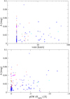 |
Fig. 5. Our amplitude of photometric variability as a function of v sini (top panel) and pEW(Hα) (bottom panel). Red crosses: ASAS data, blue triangles: MEarth, blue open circles: SuperWASP, green pluses: NSVS, magenta squares: AstroLAB IRIS, maroon C’s: ASAS-SN, black H’s: HATNet, violet K’s: K2, cyan M’s: Montcabrer, orange T’s: Montsec. |
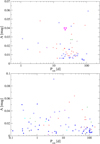 |
Fig. 6. Our amplitude of photometric variability as a function of rotation period for M0.0–M3.0 V stars (top panel) and M3.5–M8.5 V stars (bottom panel). Same symbol legend as in Fig. 5. |
Previous works have investigated the relation between A and Prot. Hartman et al. (2011) found no correlation for K and early to mid M dwarf stars if Prot < 30 d, and an anti-correlation if Prot > 30 d. They found no correlation for mid to late M dwarfs. Newton et al. (2016) analysed the MEarth sample in two groups, 0.25 M⊙ < M < 0.5 M⊙ and 0.08 M⊙ < M < 0.25 M⊙, and found an anti-correlation A − Prot in the first group and no correlation in the second group. We repeated the same exercise separating our sample in early to mid (M0.0–3.0 V; N = 63) and mid to late (M3.5–8.5 V; N = 78) stars (Fig. 6). We performed a Spearman rank correlation analysis and obtained a relation coefficient of –0.24 with p-value 0.06 for early to mid stars, and a coefficient of –0.21 with p-value 0.06 for mid to late stars. Therefore, in both cases we found a suggestive (but non-significant) anti-correlation between A and Prot. We note the overabundace of M0.0–3.0 V stars with periods Prot = 10 − 100 d with respect to M3.5–8.5 V stars).
4.4. Aperiodic variables
We also looked for aperiodic or irregular variable stars that display a large scatter in their light curves, but for which we failed to find any significant periodicity. For this reason, we used the common approach of plotting the standard deviation σ(m) of each individual light curve as a function of the mean magnitude m̅ (see e.g. Caballero et al. 2010, for a practical application). We performed this exercise for only three of the main surveys because average magnitudes of MEarth light curves were set to zero, different pass bands and instrumental set-ups must not be mixed up, and the complementary surveys and our own observations do not have enough data points for a robust analysis.
The σ(m) vs. m̅ plots for ASAS, SuperWASP, and NSVS are shown in Fig. 7. All NSVS stars follow the expected trend for their mean magnitude (see Irwin et al. 2007 for a detailed description of virtually all parameters affecting σ(m) in a photometric survey). Of the SuperWASP stars, only J09003+218 = LP 368–128, a faint M6.5 V (Dupuy & Liu 2012; Alonso-Floriano et al. 2015a), has a much larger scatter than its peers. Newton et al. (2016) found a period of 0.439 d that we did not reproduce in our datasets (Table 3). However, we attribute its large σ(m), of about 0.5 mag, to its magnitude, which is over 1 mag fainter than the second-faintest star in the SuperWASP sample. Finally, there are three outliers among the ASAS stars: J12248-182 = Ross 695, J04520+064 = Wolf 1539, J09307+003 = GJ 1125. We ascribe the origin of their large σ(m) to their short angular separation to bright background stars that contaminate the ASAS light curves. In the three cases, they are located at variable angular separations ρ ≈ 25 − 50 arcsec to stars 1.2–2.5 mag brighter in the V band than our M dwarfs. As a result, the variability observed is not intrinsic to the stars themselves.
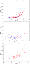 |
Fig. 7. Standard deviation σ(m) vs. mean m̅ for ASAS, SuperWASP, and NSVS magnitudes. Blue open circles and red filled circles represent stars with and without Prot computed in this work, respectively. Most of the structure, specifically in the top and bottom panels, is not of astrophysical origin but related to the different sources of noise. |
A few aperiodic or irregular variable stars also appeared in our monitoring with amateur and semi-professional telescopes. For example, with Carda we measured intra-night trends of over 0.030 mag in the known variable star J05337+019 = V371 Ori, and a 15 min, 0.030 mag-amplitude flare in the poorly investigated, X-ray emitting star J06574+740 = 2MASS J06572616+7405265.
4.5. Long-period cycles
Baliunas et al. (1996) suggested the observable Pcycle/Prot to study the relation between cycle and rotation periods. They proposed Pcycle/Prot ∼ Di, being D the dynamo number and i the slope of the relation. Slopes i ∼ 1 would imply no correlation, while values different from unity would imply a correlation between the length of the cycle and rotation period. Previous works have explored this relation (Oláh et al. 2009; Gomes da Silva et al. 2012; Suárez Mascareño et al. 2016) and find a weak correlation for F, G, and K stars. Here we repeated the exercise restricting the analysis to M dwarf stars. For this, we carefully selected 47 single, inactive M dwarfs with previous published Pcycle and Prot (Savanov 2012; Robertson et al. 2013; Suárez Mascareño et al. 2016, 2018; Wargelin et al. 2017; Küker et al. 2019) and the stars of our sample for which we have found Pcycle and Prot (see Table 2). In our sample of field M dwarfs we did not include fast-rotating, probably very young M dwarfs tabulated by Vida et al. (2013, 2014) and Distefano et al. (2016, 2017).
Figure 8 shows the plot Pcycle/Prot vs. 1/Prot in log–log scale. We found a slope i = 1.01 ± 0.06, in agreement with the results of Savanov (2012) and Suárez Mascareño et al. (2016), who also did not find a correlation between Pcycle and Prot in M dwarfs.
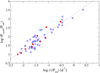 |
Fig. 8. Pcycle/Prot vs. 1/Prot in log–log scale for M dwarf stars with previous published Pcycle and Prot (blue open circles) and stars with new Pcycle from this work (red filled circles). Dashed (i = 1.01) and dotted (i = 1.00, with arbitrary offset) lines mark our sample fit and non-correlation, respectively. |
5. Conclusions
As a complement to the CARMENES survey for exoplanets, we searched for rotation periods from photometric series of 337 M dwarfs. We collected public data from long-term monitoring surveys (MEarth, ASAS, SuperWASP, NSVS, Catalina, ASAS-SN, K2, and HATNet). For 20 stars without data in these public surveys or for those with poor data, we carried out photometric monitoring in collaboration with amateur observatories. In total, we investigated 622 light curves of 334 M dwarfs. We analysed each light curve by computing LS periodograms and identifying significant signals. In some cases, we also applied GLS and Gaussian processes analyses. We found 142 signals that we interpret as rotation periods. Of these, 73 are new and 69 match or even improve previous determinations found in the existing literature. We also found long activity cycles for ten stars of the sample, six of which we report here for the first time. We explored the relation between Pcycle and Prot for a sample of 47 M dwarfs with previous reported cycle and rotation periods, and the ten M dwarfs with cycle and rotation periods presented in this work, and did not find any correlation between Pcycle and Prot.
Although the main aim of this work was to catalogue rotation periods of M dwarfs being searched for exoplanets with the radial-velocity method, and therefore to be able to discriminate between stellar activity and true exoplanet signals, we also presented results on (i) the absence of a lack of stars with intermediate periods at about 30 d with respect to stars with shorter periods in the rotation period distribution; (ii) the link between rotation period and activity, especially through rotational velocity and Hα pseudo-equivalent width; (iii) the identification of three very active, possibly young stars with new rotation periods between 0.34 d and 23.6 d; and (iv) the lack of apparent correlation between amplitude of photometric variability and Prot, v sini, and pEW(Hα).
The CARMENES Consortium will continue to improve or find new rotation periods, using them to discard or confirm radial-velocity exoplanets, and will make them public for use by other groups worldwide.
J01352–072 = Barta 161 12, J09449–123 = G 161–071.
An ultra-high-resolution spectrograph of ℛ ≳ 200 000 at an 8 m-class telescope would be needed to measure rotational velocities of a large sample of M dwarfs with an accuracy of 1 km s−1 (Reiners et al. 2018b).
Acknowledgments
We thank the anonymous referee for the careful review, F. García de la Cuesta for observing J05019+011 from Observatorio Astronómico La Vara, Luarca, Spain. CARMENES is an instrument for the Centro Astronómico Hispano-Alemán de Calar Alto (CAHA, Almería, Spain). CARMENES is funded by the German Max-Planck-Gesellschaft (MPG), the Spanish Consejo Superior de Investigaciones Científicas (CSIC), the European Union through FEDER/ERF FICTS-2011-02 funds, and the members of the CARMENES Consortium (Max-Planck-Institut für Astronomie, Instituto de Astrofísica de Andalucía, Landessternwarte Königstuhl, Institut de Ciències de l’Espai, Insitut für Astrophysik Göttingen, Universidad Complutense de Madrid, Thüringer Landessternwarte Tautenburg, Instituto de Astrofísica de Canarias, Hamburger Sternwarte, Centro de Astrobiología and Centro Astronómico Hispano-Alemán), with additional contributions by the Spanish Ministerio de Ciencia, Innovacion y Universidades (under grants AYA2016-79425-C3-1/2/3-P, AYA2017-89121-P, AYA2018-84089), the German Science Foundation (DFG), the Klaus Tschira Stiftung, the states of Baden-Württemberg and Niedersachsen, the Junta de Andalucía, and by the Principado de Asturias (under grant FC-15-GRUPIN14-017). This research made use of the SIMBAD and VizieR, operated at Centre de Données astronomiques de Strasbourg, France, and NASA’s Astrophysics Data System.
References
- Alonso, R., Brown, T. M., Charbonneau, D., et al. 2007, Transiting Extrapolar Planets Workshop, 366, 13 [Google Scholar]
- Alonso-Floriano, F. J., Morales, J. C., Caballero, J. A., et al. 2015a, A&A, 577, A128 [NASA ADS] [CrossRef] [EDP Sciences] [Google Scholar]
- Alonso-Floriano, F. J., Caballero, J. A., Cortés-Contreras, M., Solano, E., & Montes, D. 2015b, A&A, 583, A85 [NASA ADS] [CrossRef] [EDP Sciences] [Google Scholar]
- Anglada-Escudé, G., Amado, P. J., Barnes, J., et al. 2016, Nature, 536, 437 [NASA ADS] [CrossRef] [PubMed] [Google Scholar]
- Angus, R., Morton, T., Aigrain, S., Foreman-Mackey, D., & Rajpaul, V. 2018, MNRAS, 474, 2094 [NASA ADS] [CrossRef] [Google Scholar]
- Artigau, É., Kouach, D., Donati, J.-F., et al. 2014, Proc. SPIE, 9147, 914715 [CrossRef] [Google Scholar]
- Auvergne, M., Bodin, P., Boisnard, L., et al. 2009, A&A, 506, 411 [NASA ADS] [CrossRef] [EDP Sciences] [Google Scholar]
- Baliunas, S. L., & Vaughan, A. H. 1985, ARA&A, 23, 379 [NASA ADS] [CrossRef] [Google Scholar]
- Baliunas, S. L., Donahue, R. A., Soon, W. H., et al. 1995, ApJ, 438, 269 [NASA ADS] [CrossRef] [Google Scholar]
- Baliunas, S. L., Nesme-Ribes, E., Sokoloff, D., & Soon, W. H. 1996, ApJ, 460, 848 [NASA ADS] [CrossRef] [Google Scholar]
- Baluev, R. V., Sokov, E. N., Shaidulin, V. S., et al. 2015, MNRAS, 450, 3101 [NASA ADS] [CrossRef] [Google Scholar]
- Bakos, G. Á. 2018, in Handbook of Exoplanets, eds. H. J. Deeg, & J. A. Belmonte, (Springer International Publishing), 1 [Google Scholar]
- Bakos, G., Noyes, R. W., Kovács, G., et al. 2004, PASP, 116, 266 [NASA ADS] [CrossRef] [Google Scholar]
- Bakos, G. Á., Csubry, Z., Penev, K., et al. 2013, PASP, 125, 154 [NASA ADS] [CrossRef] [Google Scholar]
- Barnes, J. R., Jeffers, S. V., & Jones, H. R. A. 2011, MNRAS, 412, 1599 [NASA ADS] [CrossRef] [Google Scholar]
- Baroch, D., Morales, J. C., Ribas, I., et al. 2018, A&A, 619, A32 [NASA ADS] [CrossRef] [EDP Sciences] [Google Scholar]
- Barros, S. C. C., Faedi, F., Collier Cameron, A., et al. 2011, A&A, 525, A54 [NASA ADS] [CrossRef] [EDP Sciences] [Google Scholar]
- Berdyugina, S. V., & Järvinen, S. P. 2005, Astron. Nachr., 326, 283 [NASA ADS] [CrossRef] [Google Scholar]
- Berta, Z. K., Irwin, J., & Charbonneau, D. 2013, ApJ, 775, 91 [NASA ADS] [CrossRef] [Google Scholar]
- Boisse, I., Bouchy, F., Hébrard, G., et al. 2011, Phys. Sun Star Spots, 273, 281 [Google Scholar]
- Bonfils, X., Forveille, T., Delfosse, X., et al. 2005, A&A, 443, L15 [NASA ADS] [CrossRef] [EDP Sciences] [Google Scholar]
- Borucki, W. J., Koch, D., Basri, G., et al. 2010, Science, 327, 977 [NASA ADS] [CrossRef] [PubMed] [Google Scholar]
- Bouvier, J., Cabrit, S., Fernandez, M., Martin, E. L., & Matthews, J. M. 1993, A&A, 272, 176 [NASA ADS] [Google Scholar]
- Brown, T. M., Baliber, N., Bianco, F. B., et al. 2013, PASP, 125, 1031 [NASA ADS] [CrossRef] [Google Scholar]
- Browning, M. K. 2008, ApJ, 676, 1262 [Google Scholar]
- Browning, M. K., Basri, G., Marcy, G. W., West, A. A., & Zhang, J. 2010, AJ, 139, 504 [NASA ADS] [CrossRef] [Google Scholar]
- Butler, R. P., Vogt, S. S., Marcy, G. W., et al. 2004, ApJ, 617, 580 [NASA ADS] [CrossRef] [Google Scholar]
- Butters, O. W., West, R. G., Anderson, D. R., et al. 2010, A&A, 520, L10 [NASA ADS] [CrossRef] [EDP Sciences] [Google Scholar]
- Caballero, J. A., Cornide, M., & de Castro, E. 2010, Astron. Nachr., 331, 257 [NASA ADS] [CrossRef] [Google Scholar]
- Caballero, J. A., Cortés-Contreras, M., Alonso-Floriano, F. J., et al. 2016, 19th Cambridge Workshop on Cool Stars, Stellar Systems, and the Sun (CS19), 148 [Google Scholar]
- Chabrier, G., Gallardo, J., & Baraffe, I. 2007, A&A, 472, L17 [NASA ADS] [CrossRef] [EDP Sciences] [Google Scholar]
- Charbonneau, D., Berta, Z. K., Irwin, J., et al. 2009, Nature, 462, 891 [NASA ADS] [CrossRef] [PubMed] [Google Scholar]
- Christensen, E. J., Carson Fuls, D., Gibbs, A. R., et al. 2015, Meeting Abstr., 47, 19 [Google Scholar]
- Claudi, R., Benatti, S., Carleo, I., et al. 2016, Proc. SPIE, 9908, 99081A [CrossRef] [Google Scholar]
- Cloutier, R., Astudillo-Defru, N., Doyon, R., et al. 2017, A&A, 608, A35 [NASA ADS] [CrossRef] [EDP Sciences] [Google Scholar]
- Correia, A. C. M., Couetdic, J., Laskar, J., et al. 2010, A&A, 511, A21 [NASA ADS] [CrossRef] [EDP Sciences] [Google Scholar]
- Cortés-Contreras, M., Béjar, V. J. S., Caballero, J. A., et al. 2017, A&A, 597, A47 [NASA ADS] [CrossRef] [EDP Sciences] [Google Scholar]
- Collier Cameron, A., Bouchy, F., Hébrard, G., et al. 2007, MNRAS, 375, 951 [NASA ADS] [CrossRef] [Google Scholar]
- Collins, K. A., Kielkopf, J. F., Stassun, K. G., & Hessman, F. V. 2017, AJ, 153, 77 [NASA ADS] [CrossRef] [Google Scholar]
- Crossfield, I. J. M., Petigura, E., Schlieder, J. E., et al. 2015, ApJ, 804, 10 [NASA ADS] [CrossRef] [Google Scholar]
- Cumming, A. 2004, MNRAS, 354, 1165 [NASA ADS] [CrossRef] [Google Scholar]
- Dahn, C., Green, R., Keel, W., et al. 1985, Inf. Bull. Variable Stars, 2796, 1 [NASA ADS] [Google Scholar]
- David, T. J., Hillenbrand, L. A., Petigura, E. A., et al. 2016, Nature, 534, 658 [NASA ADS] [CrossRef] [PubMed] [Google Scholar]
- Delfosse, X., Forveille, T., Perrier, C., & Mayor, M. 1998, A&A, 331, 581 [NASA ADS] [Google Scholar]
- Distefano, E., Lanzafame, A. C., Lanza, A. F., Messina, S., & Spada, F. 2016, A&A, 591, A43 [NASA ADS] [CrossRef] [EDP Sciences] [Google Scholar]
- Distefano, E., Lanzafame, A. C., Lanza, A. F., Messina, S., & Spada, F. 2017, A&A, 606, A58 [NASA ADS] [CrossRef] [EDP Sciences] [Google Scholar]
- Dittmann, J. A., Irwin, J. M., Charbonneau, D., et al. 2017, Nature, 544, 333 [NASA ADS] [CrossRef] [Google Scholar]
- Donati, J.-F., Forveille, T., Collier Cameron, A., et al. 2006, Science, 311, 633 [NASA ADS] [CrossRef] [PubMed] [Google Scholar]
- Drake, A. J., Djorgovski, S. G., Mahabal, A., et al. 2009, ApJ, 696, 870 [NASA ADS] [CrossRef] [MathSciNet] [Google Scholar]
- Drake, A. J., Graham, M. J., Djorgovski, S. G., et al. 2014, ApJS, 213, 9 [NASA ADS] [CrossRef] [Google Scholar]
- Dressing, C. D., & Charbonneau, D. 2015, ApJ, 807, 45 [NASA ADS] [CrossRef] [Google Scholar]
- Dumusque, X., Pepe, F., Lovis, C., et al. 2012, Nature, 491, 207 [NASA ADS] [CrossRef] [PubMed] [Google Scholar]
- Dupuy, T. J., & Liu, M. C. 2012, ApJS, 201, 19 [NASA ADS] [CrossRef] [Google Scholar]
- Favata, F., Reale, F., Micela, G., et al. 2000, A&A, 353, 987 [NASA ADS] [Google Scholar]
- Fekel, F. C., & Henry, G. W. 2000, AJ, 120, 3265 [NASA ADS] [CrossRef] [Google Scholar]
- Foreman-Mackey, D., Agol, E., Ambikasaran, S., & Angus, R. 2017, AJ, 154, 220 [NASA ADS] [CrossRef] [Google Scholar]
- France, K., Froning, C. S., Linsky, J. L., et al. 2013, ApJ, 763, 149 [NASA ADS] [CrossRef] [Google Scholar]
- Freedman, D., & Diaconis, P. 1981, Probab. Theory Relat. Field, 57, 453 [Google Scholar]
- Fuhrmeister, B., Czesla, S., Schmitt, J. H. M. M., et al. 2018, A&A, 615, A14 [NASA ADS] [CrossRef] [EDP Sciences] [Google Scholar]
- Gillon, M., Pont, F., Demory, B.-O., et al. 2007, A&A, 472, L13 [NASA ADS] [CrossRef] [EDP Sciences] [Google Scholar]
- Gillon, M., Triaud, A. H. M. J., Fortney, J. J., et al. 2012, A&A, 542, A4 [NASA ADS] [CrossRef] [EDP Sciences] [Google Scholar]
- Gillon, M., Jehin, E., Lederer, S. M., et al. 2016, Nature, 533, 221 [NASA ADS] [CrossRef] [PubMed] [Google Scholar]
- Gillon, M., Triaud, A. H. M. J., Demory, B.-O., et al. 2017, Nature, 542, 456 [NASA ADS] [CrossRef] [PubMed] [Google Scholar]
- Gomes da Silva, J., Santos, N. C., Bonfils, X., et al. 2012, A&A, 541, A9 [NASA ADS] [CrossRef] [EDP Sciences] [Google Scholar]
- Greimel, R., & Robb, R. M. 1998, Inf. Bull. Variable Stars, 4652, 1 [NASA ADS] [Google Scholar]
- Hallinan, G., Antonova, A., Doyle, J. G., et al. 2008, ApJ, 684, 644 [NASA ADS] [CrossRef] [Google Scholar]
- Haro, G., & Chavira, E. 1966, Vistas Astron., 8, 89 [NASA ADS] [CrossRef] [Google Scholar]
- Hartman, J. D., Bakos, G. Á., Noyes, R. W., et al. 2011, AJ, 141, 166 [NASA ADS] [CrossRef] [Google Scholar]
- Hawley, S. L., Gizis, J. E., & Reid, I. N. 1996, AJ, 112, 2799 [NASA ADS] [CrossRef] [Google Scholar]
- Heinze, A. N., Tonry, J. L., Denneau, L., et al. 2018, AJ, 156, 241 [NASA ADS] [CrossRef] [Google Scholar]
- Herbig, G. H. 1956, PASP, 68, 531 [NASA ADS] [CrossRef] [Google Scholar]
- Herrero, E., Morales, J. C., Ribas, I., & Naves, R. 2011, A&A, 526, L10 [NASA ADS] [CrossRef] [EDP Sciences] [Google Scholar]
- Horne, J. H., & Baliunas, S. L. 1986, ApJ, 302, 757 [NASA ADS] [CrossRef] [Google Scholar]
- Howell, S. B., Sobeck, C., Haas, M., et al. 2014, PASP, 126, 398 [NASA ADS] [CrossRef] [Google Scholar]
- Irwin, J., Irwin, M., Aigrain, S., et al. 2007, MNRAS, 375, 1449 [NASA ADS] [CrossRef] [Google Scholar]
- Irwin, J., Charbonneau, D., Nutzman, P., & Falco, E. 2009, IAU Symp., 253, 37 [NASA ADS] [Google Scholar]
- Irwin, J., Berta, Z. K., Burke, C. J., et al. 2011, ApJ, 727, 56 [NASA ADS] [CrossRef] [Google Scholar]
- Jankovics, I., Tsvetkova, K. P., & Tsvetkov, M. K. 1978, Inf. Bull. Variable Stars, 1454, 1 [NASA ADS] [Google Scholar]
- Jeffers, S. V., Schöfer, P., Lamert, A., et al. 2018, A&A, 614, A76 [NASA ADS] [CrossRef] [EDP Sciences] [Google Scholar]
- Johnson, J. A., Butler, R. P., Marcy, G. W., et al. 2007, ApJ, 670, 833 [NASA ADS] [CrossRef] [Google Scholar]
- Joshi, M. M., Haberle, R. M., & Reynolds, R. T. 1997, Icarus, 129, 450 [NASA ADS] [CrossRef] [Google Scholar]
- Kaminski, A., Trifonov, T., Caballero, J. A., et al. 2018, A&A, 618, A115 [NASA ADS] [CrossRef] [EDP Sciences] [Google Scholar]
- Kiraga, M. 2012, Acta Astron., 62, 67 [NASA ADS] [Google Scholar]
- Kiraga, M., & Stepien, K. 2007, Acta Astron., 57, 149 [NASA ADS] [Google Scholar]
- Kiraga, M., & Stȩpień, K. 2013, Acta Astron., 63, 53 [NASA ADS] [Google Scholar]
- Kochanek, C. S., Shappee, B. J., Stanek, K. Z., et al. 2017, PASP, 129, 104502 [NASA ADS] [CrossRef] [Google Scholar]
- Kopparapu, R. K., Ramirez, R., Kasting, J. F., et al. 2013, ApJ, 765, 131 [NASA ADS] [CrossRef] [Google Scholar]
- Korhonen, H., Vida, K., Husarik, M., et al. 2010, Astron. Nachr., 331, 772 [NASA ADS] [CrossRef] [Google Scholar]
- Kron, G. E. 1947, PASP, 59, 261 [NASA ADS] [CrossRef] [Google Scholar]
- Küker, M., Rüdiger, G., Oláh, K., & Strassmeier, K. G. 2019, A&A, in press, DOI: 10.1051/0004-6361/201833173 [EDP Sciences] [Google Scholar]
- Léger, A., Rouan, D., Schneider, J., et al. 2009, A&A, 506, 287 [NASA ADS] [CrossRef] [EDP Sciences] [MathSciNet] [Google Scholar]
- Liebert, J., Kron, R. G., & Spinrad, H. 1978, PASP, 90, 718 [NASA ADS] [CrossRef] [Google Scholar]
- Lothringer, J. D., Benneke, B., Crossfield, I. J. M., et al. 2018, AJ, 155, 66 [NASA ADS] [CrossRef] [Google Scholar]
- Luger, R., Sestovic, M., Kruse, E., et al. 2017, Nat. Astron., 1, 0129 [Google Scholar]
- Mahadevan, S., Ramsey, L. W., Terrien, R., et al. 2014, Proc. SPIE, 9147, 91471G [NASA ADS] [CrossRef] [Google Scholar]
- Maldonado, J., Scandariato, G., Stelzer, B., et al. 2017, A&A, 598, A27 [NASA ADS] [CrossRef] [EDP Sciences] [Google Scholar]
- McCullough, P. R., Stys, J. E., Valenti, J. A., et al. 2005, PASP, 117, 783 [NASA ADS] [CrossRef] [Google Scholar]
- McQuillan, A., Aigrain, S., & Mazeh, T. 2013, MNRAS, 432, 1203 [NASA ADS] [CrossRef] [MathSciNet] [Google Scholar]
- Messina, S., & Guinan, E. F. 2002, A&A, 393, 225 [NASA ADS] [CrossRef] [EDP Sciences] [Google Scholar]
- Messina, S., Desidera, S., Turatto, M., Lanzafame, A. C., & Guinan, E. F. 2010, A&A, 520, A15 [NASA ADS] [CrossRef] [EDP Sciences] [Google Scholar]
- Mochnacki, S. W., Gladders, M. D., Thomson, J. R., et al. 2002, AJ, 124, 2868 [NASA ADS] [CrossRef] [Google Scholar]
- Mohanty, S., & Basri, G. 2003, ApJ, 583, 451 [NASA ADS] [CrossRef] [Google Scholar]
- Morin, J., Donati, J.-F., Petit, P., et al. 2008, MNRAS, 390, 567 [NASA ADS] [CrossRef] [MathSciNet] [Google Scholar]
- Mullan, D. J., & MacDonald, J. 2001, ApJ, 559, 353 [NASA ADS] [CrossRef] [Google Scholar]
- Newton, E. R., Irwin, J., Charbonneau, D., et al. 2016, ApJ, 821, 93 [NASA ADS] [CrossRef] [Google Scholar]
- Newton, E. R., Irwin, J., Charbonneau, D., et al. 2017, ApJ, 834, 85 [NASA ADS] [CrossRef] [Google Scholar]
- Norton, A. J., Wheatley, P. J., West, R. G., et al. 2007, A&A, 467, 785 [NASA ADS] [CrossRef] [EDP Sciences] [Google Scholar]
- Nutzman, P., & Charbonneau, D. 2008, PASP, 120, 317 [NASA ADS] [CrossRef] [Google Scholar]
- Ochsenbein, F., Bauer, P., & Marcout, J. 2000, A&AS, 143, 23 [NASA ADS] [CrossRef] [EDP Sciences] [Google Scholar]
- Oláh, K., Kolláth, Z., Granzer, T., et al. 2009, A&A, 501, 703 [NASA ADS] [CrossRef] [EDP Sciences] [Google Scholar]
- Osten, R. A., Hawley, S. L., Allred, J. C., Johns-Krull, C. M., & Roark, C. 2005, ApJ, 621, 398 [NASA ADS] [CrossRef] [Google Scholar]
- Osten, R. A., Godet, O., Drake, S., et al. 2010, ApJ, 721, 785 [NASA ADS] [CrossRef] [Google Scholar]
- Paunzen, E., & Vanmunster, T. 2016, Astron. Nachr., 337, 239 [NASA ADS] [CrossRef] [Google Scholar]
- Pepper, J., Pogge, R. W., DePoy, D. L., et al. 2007, PASP, 119, 923 [NASA ADS] [CrossRef] [Google Scholar]
- Pettersen, B. R., Coleman, L. A., & Evans, D. S. 1984, ApJ, 282, 214 [NASA ADS] [CrossRef] [Google Scholar]
- Pojmański, G. 1997, Acta Astron., 47, 467 [NASA ADS] [Google Scholar]
- Pojmański, G. 2002, Acta Astron., 52, 397 [Google Scholar]
- Pollacco, D. L., Skillen, I., Collier Cameron, A., et al. 2006, PASP, 118, 1407 [NASA ADS] [CrossRef] [Google Scholar]
- Queloz, D., Henry, G. W., Sivan, J. P., et al. 2001, A&A, 379, 279 [NASA ADS] [CrossRef] [EDP Sciences] [Google Scholar]
- Quirrenbach, A., Amado, P. J., Seifert, W., et al. 2012, Proc. SPIE, 8446, E0R [Google Scholar]
- Quirrenbach, A., Amado, P. J., Caballero, J. A., et al. 2014, Proc. SPIE, 9147, E1F [Google Scholar]
- Quirrenbach, A., Caballero, J. A., Amado, P. J., et al. 2015, in 18th Cambridge Workshop on Cool Stars, Stellar Systems, and the Sun, Proceedings of the Conference Held at Lowell Observatory, 8-,14 June 2014, eds. G. van Belle, & H. C. Harris, 897 [Google Scholar]
- Quirrenbach, A., Amado, P. J., Caballero, J. A., et al. 2016, Proc. SPIE, 9908, E12 [Google Scholar]
- Rasmussen, C. E., & Williams, C. K. I. 2005, Gaussian Processes for Machine Learning, (Cambridge, MA: The MIT Press) [Google Scholar]
- Reiners, A., & Basri, G. 2007, ApJ, 656, 1121 [NASA ADS] [CrossRef] [Google Scholar]
- Reiners, A., & Basri, G. 2008, ApJ, 684, 1390 [NASA ADS] [CrossRef] [Google Scholar]
- Reiners, A., & Basri, G. 2010, ApJ, 710, 924 [NASA ADS] [CrossRef] [Google Scholar]
- Reiners, A., Basri, G., & Browning, M. 2009, ApJ, 692, 538 [NASA ADS] [CrossRef] [Google Scholar]
- Reiners, A., Bean, J. L., Huber, K. F., et al. 2010, ApJ, 710, 432 [NASA ADS] [CrossRef] [Google Scholar]
- Reiners, A., Ribas, I., Zechmeister, M., et al. 2018a, A&A, 609, L5 [Google Scholar]
- Reiners, A., Zechmeister, M., Caballero, J. A., et al. 2018b, A&A, 612, A49 [NASA ADS] [CrossRef] [EDP Sciences] [Google Scholar]
- Ricker, G. R., Winn, J. N., Vanderspek, R., et al. 2015, JATIS, 1, 014003 [Google Scholar]
- Rivera, E. J., Lissauer, J. J., Butler, R. P., et al. 2005, ApJ, 634, 625 [NASA ADS] [CrossRef] [Google Scholar]
- Robertson, P., Endl, M., Cochran, W. D., & Dodson-Robinson, S. E. 2013, ApJ, 764, 3 [NASA ADS] [CrossRef] [Google Scholar]
- Saar, S. H., & Donahue, R. A. 1997, ApJ, 485, 319 [NASA ADS] [CrossRef] [Google Scholar]
- Savanov, I. S. 2012, Astron. Rep., 56, 716 [NASA ADS] [CrossRef] [Google Scholar]
- Scalo, J., Kaltenegger, L., Segura, A. G., et al. 2007, Astrobiology, 7, 85 [NASA ADS] [CrossRef] [PubMed] [Google Scholar]
- Scargle, J. D. 1982, ApJ, 263, 835 [NASA ADS] [CrossRef] [Google Scholar]
- Schwarzenberg-Czerny, A. 1991, MNRAS, 253, 198 [NASA ADS] [CrossRef] [Google Scholar]
- Segura, A., Kasting, J. F., Meadows, V., et al. 2005, Astrobiology, 5, 706 [NASA ADS] [CrossRef] [PubMed] [Google Scholar]
- Shkolnik, E., Liu, M. C., & Reid, I. N. 2009, ApJ, 699, 649 [NASA ADS] [CrossRef] [Google Scholar]
- Skrutskie, M. F., Cutri, R. M., Stiening, R., et al. 2006, AJ, 131, 1163 [NASA ADS] [CrossRef] [Google Scholar]
- Stauffer, J. R., Hartmann, L., Soderblom, D. R., & Burnham, N. 1984, ApJ, 280, 202 [NASA ADS] [CrossRef] [Google Scholar]
- Strassmeier, K. G. 2009, A&ARv, 17, 251 [NASA ADS] [CrossRef] [Google Scholar]
- Stokes, G. H., Evans, J. B., Viggh, H. E. M., Shelly, F. C., & Pearce, E. C. 2000, Icarus, 148, 21 [NASA ADS] [CrossRef] [Google Scholar]
- Suárez Mascareño, A., Rebolo, R., González Hernández, J. I., & Esposito, M. 2015, MNRAS, 452, 2745 [NASA ADS] [CrossRef] [Google Scholar]
- Suárez Mascareño, A., Rebolo, R., & González Hernández, J. I. 2016, A&A, 595, A12 [NASA ADS] [CrossRef] [EDP Sciences] [Google Scholar]
- Suárez Mascareño, A., Rebolo, R., González Hernández, J. I., et al. 2018, A&A, 612, A89 [NASA ADS] [CrossRef] [EDP Sciences] [Google Scholar]
- Tal-Or, L., Zechmeister, M., Reiners, A., et al. 2018, A&A, 614, A122 [NASA ADS] [CrossRef] [EDP Sciences] [Google Scholar]
- Tamura, M., Suto, H., Nishikawa, J., et al. 2012, Proc. SPIE, 8446, 84461T [CrossRef] [Google Scholar]
- Tarter, J. C., Backus, P. R., Mancinelli, R. L., et al. 2007, Astrobiology, 7, 30 [NASA ADS] [CrossRef] [PubMed] [Google Scholar]
- Testa, P., Drake, J. J., & Peres, G. 2004, ApJ, 617, 508 [NASA ADS] [CrossRef] [Google Scholar]
- Vida, K., Kriskovics, L., & Oláh, K. 2013, Astron. Nachr., 334, 972 [Google Scholar]
- Vida, K., Oláh, K., & Szabó, R. 2014, MNRAS, 441, 2744 [NASA ADS] [CrossRef] [Google Scholar]
- Vida, K., Kriskovics, L., Oláh, K., et al. 2016, A&A, 590, A11 [NASA ADS] [CrossRef] [EDP Sciences] [Google Scholar]
- Vida, K., Kővári, Z., Pál, A., Oláh, K., & Kriskovics, L. 2017, ApJ, 841, 124 [NASA ADS] [CrossRef] [Google Scholar]
- Wargelin, B. J., Saar, S. H., Pojmański, G., Drake, J. J., & Kashyap, V. L. 2017, MNRAS, 464, 3281 [NASA ADS] [CrossRef] [Google Scholar]
- West, A. A., Weisenburger, K. L., Irwin, J., et al. 2015, ApJ, 812, 3 [NASA ADS] [CrossRef] [Google Scholar]
- Woźniak, P. R., Vestrand, W. T., Akerlof, C. W., et al. 2004, AJ, 127, 2436 [NASA ADS] [CrossRef] [Google Scholar]
- Zechmeister, M., & Kürster, M. 2009, A&A, 496, 577 [NASA ADS] [CrossRef] [EDP Sciences] [Google Scholar]
- Zhilyaev, B. E., Romanyuk, Y. O., Verlyuk, I. A., et al. 2000, A&A, 364, 641 [NASA ADS] [Google Scholar]
Appendix A: Long tables
Tables A.1 and A.2 are available at the CDS.
Appendix B: Example light curves and periodograms
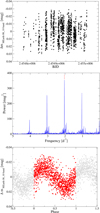 |
Fig. B.1. MEarth RG715-band photometric data (top), Lomb–Scargle periodogram (middle), and phase-folded rotation curve for P = 0.491 d (bottom) for the M5.0 V star J12189+111 = GL Vir. |
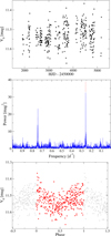 |
Fig. B.2. ASAS-3 V-band photometric data (top), Lomb–Scargle periodogram (middle), and phase-folded rotation curve for P = 3.87 d (bottom) for the M3.0 V star J03473–019 = G 080–021. |
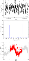 |
Fig. B.3. SuperWASP broad-band photometric data (top), Lomb–Scargle periodogram (middle), and phase-folded rotation curve for P = 4.379 d (bottom) for the M3.5 V star J22468+443 = EV Lac. |
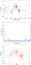 |
Fig. B.4. NSVS clear-band photometric data (top), Lomb–Scargle periodogram (middle), and phase-folded rotation curve for P = 87 d (bottom) for the M4.0 V star J23431+365 = GJ 1289. |
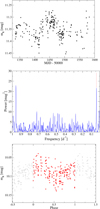 |
Fig. B.5. AstroLAB IRIS R-band photometric data (top), Lomb–Scargle periodogram (middle), and phase-folded rotation curve for P = 23.9 d (bottom) for the M3.0 V star J09428+700 = GJ 362. |
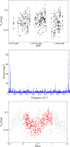 |
Fig. B.6. ASAS-SN V-band photometric data (top), Lomb–Scargle periodogram (middle), and phase-folded rotation curve for P = 32.8 d (bottom) for the M2.5 V star J20305+654 = GJ 793. |
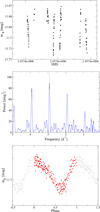 |
Fig. B.7. Montcabrer R-band photometric data (top), Lomb–Scargle periodogram (middle), and phase-folded rotation curve for P = 0.342 d (bottom) for the M5.0 V star J04772+206 = RX J0447.2+2038 (compare with Fig. B.8). |
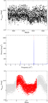 |
Fig. B.8. K2 photometric data (top), Lomb–Scargle periodogram (middle), and phase-folded rotation curve for P = 0.342 d (bottom) for the M5.0 V star J04772+206 = RX J0447.2+2038 (compare with Fig. B.7). |
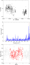 |
Fig. B.9. Montsec RC-band photometric data (top), Lomb–Scargle periodogram (middle), and phase-folded rotation curve for P = 19.3 d (bottom) for the M0.5 V star J17355+616 = BD+61 1678C. |
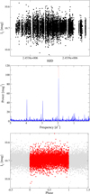 |
Fig. B.10. HATNet IC-band photometric data (top), Lomb–Scargle periodogram (middle), and phase-folded rotation curve for P = 0.512 d (bottom) for the M5.0 V star J16313+408 = G 180–060. |
All Tables
Number of investigated light curves and basic parameters of used public surveys and observatories.
All Figures
|
Fig. 1. ASAS V-band photometric data for the M0.5 V star J06105-218 = HD 42581A. It may display an activity cycle modulation with Pcycle ∼ 8.3 a superimposed to a rotation period Prot = 27.3 d (the modulation in the light curve of J15218+209 is similar). |
| In the text | |
|
Fig. 2. Periods from the literature Prot, lit as a function of our period, Prot, this work, for stars with previously published rotation periods. Dashed lines show 10% and 20% deviations from the 1:1 relation. Different symbols and colours stand for the literature source: blue crosses: Norton et al. (2007); green squares: Hartman et al. (2011); blue circles: Irwin et al. (2011); red diamonds: Kiraga (2012); brown up-triangles: Kiraga & Stepien (2007); black left-triangles: Suárez Mascareño et al. (2016); violet A’s: Newton et al. (2016); green S’s: Suárez Mascareño et al. (2018); orange asterisks: Greimel & Robb (1998), Fekel & Henry (2000), Testa et al. (2004), Rivera et al. (2005), Hallinan et al. (2008), Kiraga & Stȩpień (2013), Suárez Mascareño et al. (2015), West et al. (2015), David et al. (2016), Cloutier et al. (2017), Vida et al. (2017), and Lothringer et al. (2018). |
| In the text | |
|
Fig. 3. Distribution of rotation periods in our work (shaded, with Poissonian uncertainties) and in Carmencita (white). Rotation periods found with ASAS are shaded darker. The size of the bins follows the definitions given by Freedman & Diaconis (1981). Compare with Fig. 3 in Newton et al. (2016). |
| In the text | |
|
Fig. 4. v sini vs. Prot (top panel) and pEW(Hα) vs. Prot (bottom panel) for stars with new (blue filled circles) and re-computed rotation periods in this study (blue open circles) and stars in Carmencita with previously published rotation periods (red dots). In the top panel, the dotted lines indicate the lower and upper envelopes of the v sini − Prot relation, and most of the values at v sini = 2 or 3 km s−1 are upper limits. Compare with Figs. 6 and 8 in Jeffers et al. (2018). Here we present 154 new or improved v sini − Prot and pEW(Hα)–Prot pairs, with periods from this work and velocities and Hα equivalent widths from Reiners et al. (2018b). Outlier stars in both panels are discussed in the text. |
| In the text | |
|
Fig. 5. Our amplitude of photometric variability as a function of v sini (top panel) and pEW(Hα) (bottom panel). Red crosses: ASAS data, blue triangles: MEarth, blue open circles: SuperWASP, green pluses: NSVS, magenta squares: AstroLAB IRIS, maroon C’s: ASAS-SN, black H’s: HATNet, violet K’s: K2, cyan M’s: Montcabrer, orange T’s: Montsec. |
| In the text | |
|
Fig. 6. Our amplitude of photometric variability as a function of rotation period for M0.0–M3.0 V stars (top panel) and M3.5–M8.5 V stars (bottom panel). Same symbol legend as in Fig. 5. |
| In the text | |
|
Fig. 7. Standard deviation σ(m) vs. mean m̅ for ASAS, SuperWASP, and NSVS magnitudes. Blue open circles and red filled circles represent stars with and without Prot computed in this work, respectively. Most of the structure, specifically in the top and bottom panels, is not of astrophysical origin but related to the different sources of noise. |
| In the text | |
|
Fig. 8. Pcycle/Prot vs. 1/Prot in log–log scale for M dwarf stars with previous published Pcycle and Prot (blue open circles) and stars with new Pcycle from this work (red filled circles). Dashed (i = 1.01) and dotted (i = 1.00, with arbitrary offset) lines mark our sample fit and non-correlation, respectively. |
| In the text | |
|
Fig. B.1. MEarth RG715-band photometric data (top), Lomb–Scargle periodogram (middle), and phase-folded rotation curve for P = 0.491 d (bottom) for the M5.0 V star J12189+111 = GL Vir. |
| In the text | |
|
Fig. B.2. ASAS-3 V-band photometric data (top), Lomb–Scargle periodogram (middle), and phase-folded rotation curve for P = 3.87 d (bottom) for the M3.0 V star J03473–019 = G 080–021. |
| In the text | |
|
Fig. B.3. SuperWASP broad-band photometric data (top), Lomb–Scargle periodogram (middle), and phase-folded rotation curve for P = 4.379 d (bottom) for the M3.5 V star J22468+443 = EV Lac. |
| In the text | |
|
Fig. B.4. NSVS clear-band photometric data (top), Lomb–Scargle periodogram (middle), and phase-folded rotation curve for P = 87 d (bottom) for the M4.0 V star J23431+365 = GJ 1289. |
| In the text | |
|
Fig. B.5. AstroLAB IRIS R-band photometric data (top), Lomb–Scargle periodogram (middle), and phase-folded rotation curve for P = 23.9 d (bottom) for the M3.0 V star J09428+700 = GJ 362. |
| In the text | |
|
Fig. B.6. ASAS-SN V-band photometric data (top), Lomb–Scargle periodogram (middle), and phase-folded rotation curve for P = 32.8 d (bottom) for the M2.5 V star J20305+654 = GJ 793. |
| In the text | |
|
Fig. B.7. Montcabrer R-band photometric data (top), Lomb–Scargle periodogram (middle), and phase-folded rotation curve for P = 0.342 d (bottom) for the M5.0 V star J04772+206 = RX J0447.2+2038 (compare with Fig. B.8). |
| In the text | |
|
Fig. B.8. K2 photometric data (top), Lomb–Scargle periodogram (middle), and phase-folded rotation curve for P = 0.342 d (bottom) for the M5.0 V star J04772+206 = RX J0447.2+2038 (compare with Fig. B.7). |
| In the text | |
|
Fig. B.9. Montsec RC-band photometric data (top), Lomb–Scargle periodogram (middle), and phase-folded rotation curve for P = 19.3 d (bottom) for the M0.5 V star J17355+616 = BD+61 1678C. |
| In the text | |
|
Fig. B.10. HATNet IC-band photometric data (top), Lomb–Scargle periodogram (middle), and phase-folded rotation curve for P = 0.512 d (bottom) for the M5.0 V star J16313+408 = G 180–060. |
| In the text | |
Current usage metrics show cumulative count of Article Views (full-text article views including HTML views, PDF and ePub downloads, according to the available data) and Abstracts Views on Vision4Press platform.
Data correspond to usage on the plateform after 2015. The current usage metrics is available 48-96 hours after online publication and is updated daily on week days.
Initial download of the metrics may take a while.