| Issue |
A&A
Volume 620, December 2018
|
|
|---|---|---|
| Article Number | A135 | |
| Number of page(s) | 10 | |
| Section | Astrophysical processes | |
| DOI | https://doi.org/10.1051/0004-6361/201834131 | |
| Published online | 10 December 2018 | |
Delayed Babcock-Leighton dynamos in the diffusion-dominated regime
Leibniz-Institut für Astrophysik Potsdam (AIP), An der Sternwarte 16, 14482 Potsdam, Germany
e-mail: This email address is being protected from spambots. You need JavaScript enabled to view it.
Received:
24
August
2018
Accepted:
9
October
2018
Abstract
Context. Solar dynamo models of Babcock-Leighton type typically assume the rise of magnetic flux tubes to be instantaneous. The periods of solutions with high magnetic diffusivity are too short, and their active belts do not migrate correctly. Only the low-diffusivity regime with advective meridional flows is usually considered.
Aims. We here discuss these assumptions and apply a time delay in the source term of the azimuthally averaged induction equation. This delay is set to be the rise time of magnetic flux tubes, which are assumed to form at the tachocline. We study the effect of the delay, which adds a nonlinear temporal to the spacial nonlocality in the advective but particularly in the diffusive regime.
Methods. We have previously obtained the rise time as a function of rotation and the magnetic field strength at the bottom of the convection zone. These results allowed us to constrain the delay in the mean-field model we used in a parameter study.
Results. We identify an unknown family of solutions. These solutions show self-quenching and exhibit longer periods than their nondelayed counterparts. Additionally, we demonstrate that the nonlinear delay is responsible for the recovery of the equatorward migration of the active belts at high turbulent diffusivities.
Conclusions. By introducing a nonlinear temporal nonlocality (the delay) in a Babcock-Leighton dynamo model, we were able to obtain solutions that are quantitatively comparable to the solar butterfly diagram in the diffusion-dominated regime.
Key words: dynamo / diffusion / Sun: magnetic fields
© ESO 2018
1. Introduction
The magnetic solar cycle is attributed to a dynamo process in which motions of a conductive medium lead to the continuous induction of magnetic fields. These motions may arise from convection, which becomes anisotropic in the presence of rotation and stratification and is approximately described by the α-effect (Krause & Rädler 1980). Alternatively, they may be caused by the rise of magnetic structures to the solar surface, again in the presence of rotation and stratification, which leads to the so-called Babcock-Leighton effect (Leighton 1969). While there has been no derivation of this effect from first principles so far, the synergy with the meridional circulation in the convection zone may lead to a periodic magnetic field that satisfactorily explains the solar cycle.
Babcock-Leighton dynamos have been shown to qualitatively reproduce the solar butterfly diagram only if the turbulent magnetic diffusivity in the bulk of the convection zone is lower than 1012 cm2 s−1. This regime is often referred to as the advective regime, since the meridional circulation then determines the cycle period. In the diffusive regime, the cycle period varies with the turbulent magnetic diffusivity and can be reduced to the observed cycle length, but the propagation of the dynamo wave then follows the Parker–Yoshimura rule and is poleward at all latitudes (Yoshimura 1975).
A variety of Babcock-Leighton dynamos has been published in the past 25 years, exemplarily by Choudhuri et al. (1995), Dikpati & Charbonneau (1999), Küker et al. (2001), Chatterjee et al. (2004), Guerrero & deGouveiaDallPino(2007), and Sanchez et al. (2014) for kinematic models with stationary flows and dynamo effect, by Nandy & Choudhuri (2001) for a model with toroidal-field loss by buoyancy, and by Kitchatinov & Olemskoy (2011) for a nonlocal α-effect similar to the Babcock-Leighton effect. A nonkinematic simulation showing a solar-like butterfly diagram has been reported by Rempel (2006); here, the turbulent magnetic diffusivity rises from 1010 cm2 s−1 to 1012 cm2 s−1 in the convection zone. Beyond the Sun, Jouve et al. (2010a), for example, studied the cycle period dependence of Babcock-Leighton dynamos on the stellar rotation rate. The variability of the solar cycle including grand minima has been addressed with Babcock-Leighton dynamos for example by Karak (2010), who varied the meridional circulation, Olemskoy & Kitchatinov (2013), who varied the strength of their nonlocal source term, and Inceoglu et al. (2017), who varied both the generation of the flows and the Babcock-Leighton effect in a nonkinematic setup. In all these attempts, however, the effect of the toroidal magnetic field in the interior of the convection zone on the poloidal-field generation at the surface is instantaneous. We note that this list of papers on the Babcock-Leighton type dynamo is far from complete.
We here address the problem that the Babcock-Leighton effect is not only nonlocal in space, but also in time. Following the pioneering work by Jouve et al. (2010b), we take a further step toward a fully constrained Babcock-Leighton dynamo. Here we use the results of global numerical simulations of flux-tube rise to improve and even constrain a Babcock-Leighton dynamo model.
The global numerical simulations by Fournier et al. (2017) have shown that the rise time of magnetic flux tubes is independent of the magnetic diffusion. We suggest treating this independence with a nonlocality in space and time by designing a Babcock-Leighton dynamo model that has a time delay in the source term.
Nonlocalities have been shown to generate long-term variability in the amplitude and in the period of the magnetic cycle for a wide variety of models. A remarkable early attempt has been made by Yoshimura (1978), who used a 2D setup with source terms nonlocal in both space and time, delivering cyclic magnetic fields interrupted by “low-activity” periods that lasted for a few cycles. A sequence of papers on a 0D model, that is, without any spatial dependence but with a time delay, was published by Wilmot-Smith et al. (2006), and Hazra et al. (2014) (including stochastic variations in the Babcock-Leighton effect), and Tripathi et al. (2018), who found sub-critical dynamo action. This indicates what we show here in a 2D spherical shell with realistic solar differential rotation. It is also in line with the result by Rheinhardt & Brandenburg (2012), who studied the memory effect in a turbulent-α dynamo and found a threshold for dynamo excitation that is lower than without a memory effect. Nonlocalities in turbulent-α dynamos have been studied in various other works that we do not review here. Closest to our approach is the work by Jouve et al. (2010b), who made the time delay magnetic-field dependent. However, the authors always found that the time correlations required to obtain solar-like variability were too long to agree with the model assumptions.
Here we study such nonlocal models with time delays depending on the magnetic field strength, where the dependence is derived from the flux-rise simulations by Fournier et al. (2017). Sect. 2 describes the equations we used, and Sect. 4 shows the general results of using a delay in the induction equation. We discuss the implications of the results in Sect. 6.
2. Model and reference setup
We derived our model from Jouve et al. (2008), and like in Jouve et al. (2010b), we introduced a delay into the Babcock-Leighton source term of a mean-field dynamo. We here present the results of a large parameter study of more than 2000 simulations, which are partly constrained through the results of global numerical simulations.
The model we used here is simplified: we assumed a constant turbulent magnetic diffusivity, ηt = const, in the stellar interior. Since the turbulent diffusivity is a measure of the turbulence intensity, a constant value implies that we can neglect radial turbulent pumping (Rädler 1968). This choice was made to prevent our setup from being polluted with weakly constrained parameters, such as an arbitrary profile of the magnetic diffusivity. Observations of decaying active regions suggest that the turbulent magnetic diffusivity, ηt, at the surface is on the order of 1012 cm2 s−1, while the mixing length theory provides an upper limit of 1014cm2 s−1 at the surface and 1013 cm2 s−1 at the bottom of the convection zone. The large discrepancy between the various available estimates demonstrates the limit of our current knowledge. Additionally, a constant turbulent magnetic diffusivity has the appreciable side effect that the Reynolds number is small everywhere, allowing coarser grids and shorter computation times, which is adequate for a large parameter study.
Lengths and time were normalized with the stellar radius, R⋆, and the turbulent magnetic diffusion time,  . The free choice of the unit of the magnetic flux density B was made by setting the equipartition value with convective motions urms at r = 0.71,
  to unity, where ρ and μ0 are the gas density and the permeability constant, respectively (see below). The resulting dimensionless set of equations can be written in spherical coordinates (r, θ, ϕ) as
![Mathematical equation: $ \begin{eqnarray} \partial_t B_{\phi} ~&=&~ \left( \nabla^2 - \frac{1}{\varpi^2} \right) B_{\phi} \nonumber\\ &&~ - ~ {Re} \varpi {\bf u}_{\rm P} \cdot \nabla\left(\frac{B_{\phi}}{\varpi}\right) ~ - ~ {Re} (B_{\phi} \nabla) \cdot {\bf u}_{\rm P} \nonumber\\ &&~ + ~ C_\Omega \varpi \left[\nabla \times (\varpi A_{\phi} {\bf e}_{\phi}) \right] \cdot \nabla(\Omega) {\rm ,} \nonumber\\ \partial_t A_{\rm \phi} ~&=&~ \left( \nabla^2 - \frac{1}{\varpi^2} \right) A_{\phi} \nonumber\\ &&~ - ~ {Re} \frac{{\bf u}_{\rm P}}{\varpi} \cdot \nabla (\varpi A_{\phi}) ~ + ~ C_{S} S {\rm ,} \end{eqnarray} $](/articles/aa/full_html/2018/12/aa34131-18/aa34131-18-eq3.gif) (1)
(1)
with Bϕ, uP, ϖ, Aϕ, Ω and S, being the azimuthal magnetic flux density, the meridional circulation profile, the cylindrical distance to the rotation axis, the vector potential of the poloidal magnetic field, the angular velocity, and the source term for the poloidal field, respectively.
This system is controlled by three dimensionless parameters, the Reynolds numbers for the rotation and the meridional flow, CΩ and Re, and the dynamo number CS,
 (2)
(2)
with u0, Ω0, and S0 being the maximum meridional velocity, angular velocity, and Babcock-Leighton effect, respectively. The profiles of uP and Ω are normalized by u0 and Ω0, respectively.
The loose constraint on the amplitude and the profile of the meridional circulation gives some freedom for the choice of Re. The original model used a canonical profile aimed at representing the general characteristics of the solar flows. However, the profile remained arbitrary, and the surface shear layer was missing. We suggest to take advantage of the results of Küker & Rüdiger (2011): the authors provide consistent profiles of differential rotation and meridional flows based on the Λ-effect theory (Rüdiger 1989). This theoretical result provides a solar-like profile including a surface shear layer, with a single free coefficient whose value is set to fit the helioseismic observations. The differential rotation together with the meridional circulation profiles and amplitudes are illustrated in Fig. 1.
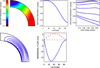 |
Fig. 1. Solar-like differential rotation and meridional circulation obtained from a mean-field hydrodynamic simulation (Küker & Rüdiger 2011). |
In Babcock-Leighton dynamos, the source term S is based on phenomenological arguments. Observations suggest that the reversed polarity of the poloidal field emerging at the surface leads to a reversal of the large-scale polar magnetic field. The source term S is an attempt to represent the physical processes that generate the poloidal field from the deeply seated toroidal field.
In the traditional frame of the Babcock-Leighton effect, buoyancy transports toroidal magnetic flux to the surface for sufficiently strong magnetic fields. During its rise through the convection zone, a poloidal field can be generated under the action of the Coriolis effect, which then provides the necessary field at the surface for the Babcock-Leighton effect to work. Global simulations were able to show that buoyant magnetic structures locally quench the magnetic turbulent diffusivity, ηt, allowing them to remain coherent throughout their rise (Cattaneo & Hughes 1988). Additionally, Fan et al. (1994) showed that the solar meridional flow does not significantly affect the rise of magnetic flux tubes. Therefore, the buoyant transport of magnetic flux is independent of ηt and of the meridional flow, uP, and exclusively depends on the magnetic pressure, that is, on B.
In the model presented here, we treat the transport independence of ηt as a memory effect in the mean-field equations. The source of the poloidal field at the surface is correlated with the toroidal field at the bottom of the convection zone at an earlier time. The considered time correlation, τdelay, represents the time required by a buoyant magnetic structure to rise from the bottom of the convection zone to the surface.
We write the delayed source term as
![Mathematical equation: $ \begin{align} & S(r, \theta, t) = f(r,\theta) \sum_{\tau_{i}} \left\{ \left[ 1 + \left( B_{\phi}(r_0, \theta, t - \tau_{i}) / B_{\rm quench} \right)^2 \right]^{-1}\right.\nonumber\\ & \qquad\qquad\quad\phantom{f(r,\theta) \sum_{\tau_{i}}} B_{\phi}(r_0, \theta, t - \tau_{i}) \Bigg\}{\rm ,} \nonumber\\ &{\rm for}\quad B_{\phi}(r_0, \theta, t - \tau_{i}) > B_{\rm threshold} {\rm ,}~ S=0~{\rm otherwise.} \end{align} $](/articles/aa/full_html/2018/12/aa34131-18/aa34131-18-eq5.gif) (3)
(3)
Here the sum is computed over all magnetic flux tubes that reach the surface at a given time t.
On the one hand, tubes with magnetic flux densities higher than Bquench are weakly affected by the Coriolis effect and emerge as untilted active regions (D’Silva & Choudhuri 1993; Jouve et al. 2013; Fournier et al. 2017). Such untilted regions do not provide poloidal magnetic flux to the Babcock-Leighton effect. On the other hand, weak flux tubes may be strongly affected by the turbulent convective motions such that they do not reach the surface. We consider a threshold, Bthreshold, below which the toroidal field does not participate in the dynamo mechanism. Such a lower limit prevents the dynamo from growing from an arbitrarily low seed field.
Since the place where the source S operates remains unknown, we used the same arbitrary profile as Jouve et al. (2008), where S is nonzero at r ≳ 0.9 and is maximum at 45° latitude at the surface,
![Mathematical equation: $ \begin{equation} f(r, \theta) = \frac{1}{2} ~ \left[ 1 + {\rm erf} \left( \frac{ r - 0.9 }{0.02} \right) \right] \cos \theta \sin \theta{\rm .} \end{equation} $](/articles/aa/full_html/2018/12/aa34131-18/aa34131-18-eq6.gif) (4)
(4)
2.1. Introducing the 3D results into the model
Global simulations have enabled us to constrain the correlation time, τdelay, the source-term quenching, Bquench, and the magnetic field threshold, Bthreshold. Here τdelay represents the rise time of magnetic flux tubes, that is, coherent magnetic structures that may form from the destabilization of a previously amplified magnetic layer (Rempel & Schüssler 2001; Hotta et al. 2012) by the buoyancy instability (Parker 1955; Matthews et al. 1995; Wissink et al. 2000; Fan 2001; Kersalé et al. 2007; Favier et al. 2012). The amplification only depends on the stratification of the solar convection zone and has been found to be Famp = 10 (Rempel & Schüssler 2001; Hotta et al. 2012). As a result, amplified flux tubes can reach up to 15 × 104 G (i.e., 10 Beq).
Fournier et al. (2017) demonstrated that the rise time of magnetic flux tubes follows the relation
 (5)
(5)
where Prot is the rotation period of the star, and  is the ratio between the buoyant force and the Coriolis effect, modified by the magnetic tension. The exponent α3 is a function of the azimuthal mode number with which the magnetic flux tube rises. In the case of the Sun, taking Prot constant, this relation reduces to
 (6)
(6)
with α varying between −0.91 and −2.0 depending on the azimuthal mode. The parameter τ0 is the rise time for a field in equipartition with the convective velocity, Bϕ = Beq , and is a free parameter. It depends on the rotation period of the star, the depth of its convection zone, and the details of the destabilization process forming the flux tubes as well as on the profiles of the turbulent thermal conductivity, viscosity, and diffusivity.
In Eq. (6) there is no latitudinal dependence. Recalling that this equation describes the reduction of the rise velocity by the tension force, however, we can model it following the latitudinal dependence of the tension force of 1/sin θ,
 (7)
(7)
We further define an effective delay τeff, which is a very useful parameter. It corresponds to the shortest delay in any given moment, that is,
 (8)
(8)
where  is the strongest field strength generated by the Ω-effect at the bottom of the convection zone. The maximum is taken over time and latitude (after saturation).
Rempel (2006) showed that Babcock-Leighton dynamos provide Bϕ up to 3Beq. Since the resulting amplified flux tubes are in the buoyancy-dominated regime and therefore weakly participate in the dynamo because the Coriolis effect is not strong enough for significantly tilted active regions (see the appendix), we set Bquench = 3Beq. Fan et al. (2003) have shown that amplified flux tubes weaker than 3Beq will not reach the surface as coherent structures. The lower threshold on Bϕ is Bthreshold = 3Beq/Famp = 0.3Beq. Since magnetic flux tubes of threshold flux density may have rise times on the order of a cycle, we implemented a source term buffer that lasted until t + 5 τdiff for any moment t in the simulation, in order to prevent any issues with very long delays.
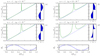 |
Fig. 2. Zero-dimensional toy model illustrating the effect of the delay. In each panel the green curve represents the evolution of the delay with time for a given Bϕ, indicated in the lower panels as the blue curve. The dashed line represents time. The histogram on the right-hand side represents the resulting source term S normalized in arbitrary units. Panels a and b illustrate the case of a weakly nonlinear delay (α = −1), and panels c and d show a nonlinear delay (α = −2). Panels a and c show a short effective delay (e.g., |

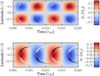 |
Fig. 3. Color-coding of the toroidal magnetic field strengths of an artificial oscillatory dipole (top panel) and an artificial oscillatory quadrupole (bottom panel). The contours represent the source term (S) at the surface for α = −2 and τ0 = 10−2Pcyc. |
2.2. Behavior of the delay
The dependence of the delay on Bϕ is controlled by α. When α is set to zero, the delay is constant. A constantly delayed source term has the same time-profile as a non-delayed source term, but is shifted in time. However, as soon as α becomes nonzero, the delay becomes time dependent. Weaker flux tubes rise longer than stronger ones. Weak flux tubes may therefore reach the surface at the same time as stronger flux tubes that formed at a later time. The time-dependence of the delay results in an accumulation of the source at the surface at certain times.
We illustrate this behavior in Fig. 2 for four different idealized cases. We consider a single point with a sinusoidally varying toroidal magnetic field,
 (9)
(9)
with amplitude  and frequency ω. The field is shown as blue curves in Fig. 2, while the red curves are the delay computed from Bϕ. The histograms show the resulting source of poloidal field accumulated from Bϕ in the past. The two upper panels show the case of a weakly nonlinear short- and a long-τeff, respectively (with α = −1). The two lower panels illustrate a strongly nonlinear short- and long-τeff (with α = −2). In the weakly nonlinear short-τeff case, the accumulation seen in the diagram is almost negligible and the time-profile of the source looks almost identical to the profile of Bϕ. Only for a longer τeff does the accumulation become visible. A similar accumulation is found for the nonlinear short-τeff, demonstrating that the nonlinearity support the accumulation. In the case of the long-τeff , the deformation of the profile leads to a front.
Clearly, two aspects of the delay lead to accumulation: the length of the effective delay, τeff, controlled by τ0 and  , and its nonlinearity, controlled by α.
Because of the latitudinal dependence of the toroidal magnetic field, the delay naturally varies with latitude. Like its time dependence, the latitudinal dependence of the delay is a function of α and τ0, but it additionally depends on the sign of the latitudinal gradient of the toroidal field, ∂Bϕ/∂θ. Figure 3 shows that if the toroidal field decreases toward the equator, the resulting delayed field, illustrated by the contour plots, migrates equatorward, whereas when the gradient is directed poleward, the dynamo wave propagates poleward because weaker fields rise on a longer timescale and the accumulation is delayed, which sets the direction of propagation with the latitudinal gradient of Bϕ.
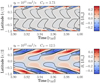 |
Fig. 4. Radial magnetic field at the surface as a function of time from the solutions in the advection-dominated regime (ADV, top panel) and the diffusion-dominated regime (DIFF, bottom panel). Contours also represent Br, but show the 15, 1.5, and 0.15% levels of |


3. Nondelayed model
We solve Eq. (1) with the pseudo-spectral spherical code by Hollerbach (2000), in which the diffusion term is solved in spectral space, but the induction term is solved in real space. We do not employ the momentum and temperature equations of the code here. The induction equation solution took part in the benchmark by Jouve et al. (2008), and after implementing the delay term for the present study, we confirmed their results for τdelay = 0, as shown in Fig. 4. Our constant turbulent diffusivity of ηt = 1011 cm2 s−1 as compared to the radius-dependent diffusivity in the benchmark, and our theory-based differential rotation versus the closed approximation in the benchmark do not modify the overall picture of the solutions. The slight difference in the amplitude of the meridional flow, due to the theoretical profile, explains the longer magnetic cycle of 40 yr compared to 30 yr of Jouve et al. (2010b). The solution is antisymmetric and oscillatory, with concentrated strong polar regions and rather weak magnetic fields at low latitudes, which are about 10−3 of the high-latitude fields, migrating equatorward. The model is labeled ADV in Table 1 and falls short of producing strong enough low-latitude toroidal fields for a realistic solar butterfly diagram. Another issue is the cycle, which remains too long.
This solution is located in the advection-dominated regime, where the magnetic cycle mostly depends on the meridional circulation. The meridional circulation amplitude is defined as a byproduct of the Λ-effect that reproduces the solar differential rotation and only requires the mixing length parameter αMLT. This means that the only possibility to decrease the magnetic cycle in this setup is to increase the turbulent magnetic diffusion toward the diffusion-dominated regime.
It is well known that dynamo solutions in the advection-dominated regime differ from those in the diffusion-dominated regime. In the lower panel of Fig. 4, we show a model in the diffusion-dominated regime, with ηt = 1012 cm2 s−1. The relevant parameters are listed in Table 1 under the label DIFF. The solution remains antisymmetric and oscillatory, with an activity-cycle period of 8 yr. The polar regions are less concentrated, more similar to the solar characteristics, and the low latitudes exhibit stronger fields (≈10% of the high-latitude fields), but the dynamo wave propagates purely radially, as predicted by the Parker–Yoshimura rule.
Even if an ηt exists for which the nondelayed model gives a solution with an 11-year cycle period, the low-latitude radial fields remain weaker than the polar regions, and the migration becomes radial while moving to the diffusion-dominated regime.
4. Recovering the solar characteristics with the delay model
We modeled the rise time as a temporal nonlocality, the delay, because Fournier et al. (2017) have shown in global simulations of rising magnetic flux tubes that the rise time is independent of the turbulent magnetic diffusion. In Sect. 2.2 we have shown that a time-dependent delay leads to temporal peaks in the source term S of the induction equation near the surface, migrating latitudinally in the direction of decreasing toroidal field. We show below that the solar characteristics can only be recovered in the diffusive regime (model D-DIFF). We present one series of simulations in the advection-dominated regime (D-ADV) and another one in the diffusion-dominated regime (D-DIFF). In both series, CS and τ0 are varied. Since we found that the accumulation is largest in the nonlinear regime, we present two series with α = −2. The parameters Re and CΩ are both fixed by the differential rotation profile, whose shape is determined by the Λ-effect and a standard solar model. Bquench and Bthreshold are both constrained by the results of Fournier et al. (2017) and Famp by Hotta et al. (2012). The two remaining parameters are CS and τ0. They are not yet constrained by any global simulation results. We have seen that τ0 may determine the variability of S, and CS may determine its amplitude. The parameters are summarized in Table 1.
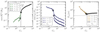 |
Fig. 5. D-ADV case. Saturation field strength (left panel), effective delay (middle panel), and cycle period (right panel) as functions of the source term amplitude CS for four different delays. Each line represents a series of runs for a given delay. The vertical solid line marks the critical |

Parameters of the various setups.
4.1. Advection-dominated case
In this section we consider the ADV setup in the advection-dominated regime, with ηt = 1011 cm s−1. In the left panel of Fig. 5, we illustrate the maximum of the toroidal magnetic field at the bottom of the convection zone,  , against CS. The nondelayed series with τ0 = 0 shows a critical source term amplitude of
  below which the model produces decaying solutions. It is remarkable that delayed dynamos deliver nondecaying solutions for weaker CS than
  . The delay has the surprising effect of reducing the criticality of the dynamo, opening a window to unknown solutions.
These solutions have the particular property of self-saturating at low amplitudes. The nonlinearity of the delay acts as a quenching mechanism, which is appealing since the solutions become independent of the model used for the quenching.
The middle panel of Fig. 5 illustrates the dependence of the relative effective delay (τeff/Pcyc) on τ0 and CS. In this figure we identify two different regimes: the short-τeff and the long-τeff regime.
In the short τeff regime, the effective delay is several orders of magnitude shorter than the cycle period and therefore produces solutions that are almost identical to the nondelayed case. Some accumulation is visible at mid-cycle (compare the top panels of Figs. 4 and 6) for strongly nonlinear delays (α = −2), but disappears for weaker nonlinearity with α = −1. The cycle period is independent of CS , as also shown in Fig. 5.
The second regime we identify is the long-τeff regime, which is characterized by a τeff between 10−3 Pcyc and 10−1 Pcyc. This domain corresponds to the delay expected in the solar case (between a few days and a few months) and is therefore the regime of interest. The solutions self-saturate, which leads to a strong dependence of the saturation field and of the cycle period on CS. The cycle period is also shown to be an increasing function of τeff.
It appears that the transient peaks in S at the surface provide a sufficient source to maintain a dynamo that would otherwise decay. Therefore the saturation mechanism is not the quenching of the source term, but the balance between the diffusion and the regular peaks of the accumulated source term S. We still do not understand why an increase of the effective delay (lower CS) increases the cycle period.
Jouve et al. (2010b) studied the effect of τ0 for a given  . Here we demonstrate that the delay reduces
  and identify two regimes. We studied the effect of τ0 for each regime and extended the analysis of Jouve et al. (2010b).
In Fig. 5, it is remarkable that the effective delay and the cycle period are independent of τ0. The long-τeff regime results from the nonlinearity of the delay, controlled by α. Fournier et al. (2017) showed that α is a function of the azimuthal mode with which an unstable flux tube rises. Determining under which condition one or the other mode is preferred will provide solid input to constrain this parameter.
Figure 6 illustrates the radial field at the surface in the long- and short-τeff regimes. In both regimes the morphological characteristics of the delayed dynamo resemble the nondelay case: at high latitudes, the strong polar fields are concentrated close to the pole, propagating poleward; at low latitude, the radial fields remain weak, showing an equatorward propagation. Even though the accumulation in S increases the field strength at low latitudes, it remains two orders of magnitude weaker than the polar fields.
Additionally, in the short-τeff regime, the cycle period remains exclusively controlled by the meridional circulation, like in the nondelayed solutions, but in the long-τeff regime, the cycle period clearly increases, with decreasing CS.
We conclude that the nonlinear delay does not affect the qualitative characteristics of the dynamo, but by increasing the cycle period, renders it a worse quantitative result. We summarize the dynamo characteristics in Table 2.
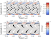 |
Fig. 6. Radial magnetic field at the surface as a function of time from the advection-dominated case with delay (D-ADV) for two source term amplitudes CS. The respective parameters are indicated above the plot. The black solid lines represent the 1.5 and 0.15% levels of |

4.2. Diffusion-dominated case
Estimates of the turbulent magnetic diffusivity from observations and mixing-length-based stellar models suggest a value higher than 1012 cm2 s−1. However, as seen in the lower panel of Fig. 4 for the nondelayed case in the diffusive regime, even though the cycle period of about 8 yr fits the observations better, the low latitudes remain weakly active and the dynamo wave propagates radially. The fact that turbulent magnetic diffusivities lower than 1012 cm2 s−1 are required in order to obtain an equatorward migration has been a long-standing issue in Babcock-Leighton dynamos.
In Sect. 2.2 we have shown that for a prescribed sinusoidal magnetic field, the maximum field propagates in the latitudinal direction of the magnetic gradient. Here we discuss this mechanism for the simulated results.
As in the advection-dominated regime, the introduction of the delay reduces the criticality of the dynamo and opens a window for new types of solutions. We could also identify the same regimes, illustrated in Fig. 7. The short-τeff regime remains identical to the nondelayed case, and shows the same differences to the solar cycle (upper panel of Fig. 8). In the long-τeff regime the overall behavior is similar: the cycle period and the effective delay are independent of τ0. The solutions saturate before reaching Bquench (left panel), and the cycle period decreases with CS (right panel). However, the morphologic characteristics of the dynamo are clearly different. The lower panels of Fig. 8 show that the reduction of criticality allows an accumulation of Br that reaches ≈25% of the polar region field strength. Furthermore, the latitudinal distribution of the initial magnetic field (decreasing toward the equator) leads to an equatorward propagation in the low latitudes. The last panel of Fig. 8 shows a solution that quantitatively agrees with the solar characteristics (see Table 2).
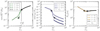 |
Fig. 7. D-DIFF case. Saturation field strength (left panel), effective delay (middle panel), and cycle period (right panel) as functions of the source term amplitude CS for four different delays. Each line represents a series of runs for a given delay. The vertical solid line marks the critical |

Dynamo characteristics.
In this particular run, τeff = 3 × 10⁻³ Pcyc , which is about a few days. Solutions with effective delays of up to a few months show comparable behaviors, however. This shows that the nonlocality introduces an additional timescale on the order of days, which is sufficient to obtain accumulation of radial-flux generation at low latitudes and equatorward migration.
4.3. Comparison to the solar case
The series we carried out in the diffusion-dominated regime shows a good quantitative agreement with the solar case, but we scanned the constrained parameter space with the remaining free parameters, namely ηt, τ0 , and CS, and selected a simulation that we call SOLAR, which reproduces the solar characteristics. By varying CS and ηt, we were able to find dynamo solutions whose butterfly diagram quantitatively matches several characteritics of the solar observations. We summarize these aspects in Table 2. We compared the activity cycle period, the propagation of the active belt and the high latitude, the extent of the polar regions, and the activity level of the low latitudes. We recall that the averaged strength of the observed active belts is about an order of magnitude weaker than the polar field strength.
The SOLAR solution is antisymmetric and oscillatory, with a cycle of 11 yr, an extent of the polar regions of 36° , the amplitude of the low latitudes is a fourth of the amplitudes of the polar regions, and an equatorward propagation of the active belt as well as a poleward propagation of the high-latitude fields. It is also remarkable that the polar reversal occurs at half-cycle of the low latitude. The turbulent magnetic diffusivity required to obtain this solution is ηt = 6.7 × 1011 cm2 s−1, which is in the transitional regime between the diffusive and the advective regime. The resulting effective delay τeff is on the order of a month (≈33 days). The toroidal field at the bottom of the convection zone saturates below equipartition with the convective motions, at about 0.15 Beq.
In Fig. 9 we illustrate various aspects of the dynamo mechanism, showing how the toroidal field profile (a) is distorted into a source term sharply peaked in time (b), building up a front that, added to the diffuse field at the surface, leads to the very characteristics of the butterfly diagram (c). Because of the stiff accumulation, the active latitudes are more strongly localized in latitude and time than the solar butterfly diagram. As Weber et al. (2011) have shown that convective motions introduce stochasticity in the emergence characteristics of active regions, this mechanism could explain the broadening of the real solar activity bands in the butterfly diagram. We illustrate the propagation of the active latitudes in the meridional plane in Fig. 10, where the solid and dashed black contours represent the toroidal field, and the color-coding shows the negative and positive radial field strength, respectively. The slices are taken in the beginning of the activity cycle, at maximum, in the decreasing phase, and at minimum. The toroidal field peaks at high latitudes and propagates almost radially, as predicted by the Parker–Yoshimura rule. The strongest radial field is located at the pole. Close to the surface, where the source term is the strongest, the active latitudes, indicated by the dashed ovals, can be seen to migrate to the equator. These meridional sections demonstrate that the equatorward migration of the active belt does not follow the migration of the dynamo wave, which propagates almost radially, but is caused by the longer delay for weaker toroidal fields closer to the equator.
5. Sensitivity of the results to the free parameters
Since some parameters remain weakly or even not constrained, it is important to discuss the reliability of the results of the previous section. The accumulation of the source term S in short-lived peaks as a result of the delay is the key aspect of the model and provides the solar-like characteristics. For a prescribed oscillating magnetic field, the accumulation is controlled by the two parameters τ0 and α (see Sect. 2.2). Fournier et al. (2017) were able to constrain α in the range of −0.91 to −2 depending on the unstable azimuthal mode of the rising flux tube. However, one of the limitations of the latter work is the lack of constraint on τ0. It depends on many details of the formation of magnetic flux tubes and will be clearly challenging to constrain. Fortunately, we were able to demonstrate that the actual solutions in the long-τeff regime are clearly independent of τ0. As for the dependence on α, we have varied α from −2 to −0.1 and found that solar-like solutions could be obtained until α = −1, which remains within the above constrained space. For −1 < α, the accumulation is not sufficient and the dynamo decays.
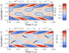 |
Fig. 8. Radial magnetic field at the surface as a function of time from the diffusion-dominated case with delay (D-DIFF) for |


Even though we were able to constrain the value of Bquench in the first term in the sum of Eq. (3) based on global numerical simulations, the quadratic quenching we use is quite arbitrary. Because this model possesses the surprising capability of self-quenching through its nonlinear nonlocality, however, the solutions are independent of the chosen quenching model. The level of saturation only depends on the effective delay, τeff, which is an outcome of the model and cannot be chosen arbitrarily.
Because we use a lower threshold on the magnetic field, some mode may not grow. The preferred mode of the dynamo is determined by the choice of the threshold and the initial condition. Although the threshold is relatively well constrained from the stability analysis of the buoyancy instability (Ferriz-Mas et al. 1994), it prevents the dynamo from growing from an arbitrary low seed field.
As is expected for the diffusion-dominated regime, the cycle period depends on ηt, but in contrast to the nondelayed dynamos, the delayed model additionally shows a dependence on CS. The cycle period may change by a factor of two over the relevant range of CS. This is remarkable because it might explain how solar-like stars with a comparable rotation period and convective envelope (same ηt) could show different magnetic cycles, which might be due to a difference in metalicity, for instance. This dependence needs to be carefully addressed because the interpretation of CS as a physical quantity is not trivial. More global simulations are required to be conclusive on this issue. The nonlocal dynamos seem to be good candidates to address this particular issue, however.
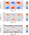 |
Fig. 9. Results of the SOLAR setup, with the color-coded toroidal magnetic field at the bottom of the convection zone (panel a), the resulting delayed source term at the surface (panel b), and the radial magnetic field at the surface (panel c). Contours in panel c represent the 25% level of |

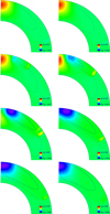 |
Fig. 10. Slices of the northern hemisphere. The slices are taken at different phases of the cycle, ordered from left to right and top to bottom panels: the rising phase, the maximum phase, the declining phase, and the minimum of the activity cycle. The colored contours represent the radial magnetic field, with red pointing outward and blue inward. Contours are 5% and 2.5% of the maximum Bϕ. |
6. Conclusions
Until now, diffusive Babcock-Leighton dynamos were considered to be unable to qualitatively reproduce the solar dynamo. The Parker–Yoshimura rule implies for the internal differential rotation of the Sun that the dynamo wave propagates poleward. We also find that the cycle period is too short and the low-latitude radial fields are too weak.
We here introduced a delay in the source term of the poloidal field. Like in Jouve et al. (2010b), this delay represents the rise time of magnetic flux tubes through the convection zone. In contrast to previous studies, however, we built this model on the results of global numerical simulations of rising magnetic flux tubes in compressible stellar interiors (Fournier et al. 2017). The model consists of a rise time that depends nonlinearly on the magnetic flux density.
We have shown that the nonlinearity of the delay leads to an accumulation of the Babcock-Leighton source term at certain times. When this accumulation becomes sufficiently important, it may prevent the dynamo from decaying, even though the nondelayed model shows no dynamo action. The reduction of the criticality of the dynamo opens a new window to unknown solutions. These delayed dynamos have the peculiar property of self-quenching.
We found that the nonlinear delay can provide a mechanism for generating a migration of the surface fields in the direction of weaker internal fields. In case of a stationary toroidal internal field at mid-latitudes, for example, the generated poloidal fields at the surface migrate toward the equator at low latitudes and toward the poles at high latitudes. This is independent of the sign of the internal differential rotation.
The requirement of a low turbulent magnetic diffusivity, ηt, for Babcock-Leighton dynamos to qualitatively reproduce the solar cycle has been shown to be unnecessary. We demonstrated that our delayed model, with a turbulent magnetic diffusivity of ηt = 6.7 × 1011 cm2 s−1, agrees well with the solar butterfly diagram, even though the diffusivity is relatively high throughout the entire convection zone.
We note that one proposed solution of the low-diffusivity problem is to use different values for ηt for the toroidal and for the poloidal components in the induction equation (Chatterjee et al. 2004). While the diffusivity may well be different in the horizontal and vertical directions, the poloidal field has varying components in both the horizontal and vertical directions, rendering the poloidal-field diffusivity location dependent. We have not tried such a setup, and it may not be necessary given the results we presented.
The model we presented is by design a simplified model. It has allowed us to identify the effect of the delay on the dynamo solutions. However, several ingredients are lacking for a state-of-the-art model (Rempel 2006; Cameron & Schüssler 2015; Pipin 2017). We only solved the induction equation for large-scale fields. We ignored turbulent pumping and back-reaction of the magnetic field on the flow. All these elements will increase the complexity of the model and add more free parameters that need to be constrained.
The large-scale field generation based on the Babcock-Leighton effect has not been derived from first principles. Its validity therefore remains uncertain. In the absence of global simulations addressing the formation of magnetic flux tubes, the current models remain quite arbitrary. Nevertheless, the nonlinearities of our solutions are potentially relevant for dynamos other than those of Babcock-Leighton type.
Finally, the relevance of this work for stellar dynamos will be revealed only if this model is proven to reliably reproduce observed dynamo patterns of other solar-like stars.
Acknowledgments
We would like to thank the participants and organizers of the Natural Dynamos (2016) conference for constructive remarks and input.
References
- Cameron, R., & Schüssler, M. 2015, Science, 347, 1333 [NASA ADS] [CrossRef] [Google Scholar]
- Cattaneo, F., & Hughes, D. W. 1988, J. Fluid Mech., 196, 323 [NASA ADS] [CrossRef] [Google Scholar]
- Chatterjee, P., Nandy, D., & Choudhuri, A. R. 2004, A&A, 427, 1019 [NASA ADS] [CrossRef] [EDP Sciences] [Google Scholar]
- Choudhuri, A. R., Schussler, M., & Dikpati, M. 1995, A&A, 303, L29 [NASA ADS] [Google Scholar]
- Dikpati, M., & Charbonneau, P. 1999, ApJ, 518, 508 [NASA ADS] [CrossRef] [Google Scholar]
- D’Silva, S., & Choudhuri, A. R. 1993, A&A, 272, 621 [NASA ADS] [Google Scholar]
- Fan, Y. 2001, ApJ, 546, 509 [NASA ADS] [CrossRef] [Google Scholar]
- Fan, Y., Fisher, G. H., & McClymont, A. N. 1994, ApJ, 436, 907 [NASA ADS] [CrossRef] [Google Scholar]
- Fan, Y., Abbett, W. P., & Fisher, G. H. 2003, ApJ, 582, 1206 [NASA ADS] [CrossRef] [Google Scholar]
- Favier, B., Jouve, L., Edmunds, W., Silvers, L. J., & Proctor, M. R. E. 2012, MNRAS, 426, 3349 [NASA ADS] [CrossRef] [Google Scholar]
- Ferriz-Mas, A., Schmitt, D., & Schuessler, M. 1994, A&A, 289, 949 [NASA ADS] [Google Scholar]
- Fournier, Y., Arlt, R., Ziegler, U., & Strassmeier, K. G. 2017, A&A, 607, A1 [NASA ADS] [CrossRef] [EDP Sciences] [Google Scholar]
- Guerrero, G. A., & de Gouveia Dal Pino, E. M. 2007, Astron. Nachr., 328, 1122 [NASA ADS] [CrossRef] [Google Scholar]
- Hazra, S., Passos, D., & Nandy, D. 2014, ApJ, 789, 5 [NASA ADS] [CrossRef] [Google Scholar]
- Hollerbach, R. 2000, Int. J. Numer. Meth. Fluids, 32, 773 [CrossRef] [Google Scholar]
- Hotta, H., Rempel, M., & Yokoyama, T. 2012, ApJ, 759, L24 [NASA ADS] [CrossRef] [Google Scholar]
- Inceoglu, F., Arlt, R., & Rempel, M. 2017, ApJ, 848, 93 [Google Scholar]
- Jouve, L., Brun, A. S., Arlt, R., et al. 2008, A&A, 483, 949 [NASA ADS] [CrossRef] [EDP Sciences] [Google Scholar]
- Jouve, L., Brown, B. P., & Brun, A. S. 2010a, A&A, 509, A32 [NASA ADS] [CrossRef] [EDP Sciences] [Google Scholar]
- Jouve, L., Proctor, M. R. E., & Lesur, G. 2010b, A&A, 519, A68 [NASA ADS] [CrossRef] [EDP Sciences] [Google Scholar]
- Jouve, L., Brun, A. S., & Aulanier, G. 2013, ApJ, 762, 4 [NASA ADS] [CrossRef] [Google Scholar]
- Karak, B. B. 2010, ApJ, 724, 1021 [NASA ADS] [CrossRef] [Google Scholar]
- Kersalé, E., Hughes, D. W., & Tobias, S. M. 2007, ApJ, 663, L113 [NASA ADS] [CrossRef] [Google Scholar]
- Kitchatinov, L. L., & Olemskoy, S. V. 2011, Astron. Nachr., 332, 496 [NASA ADS] [CrossRef] [Google Scholar]
- Küker, M., & Rüdiger, G. 2011, Astron. Nachr., 332, 933 [NASA ADS] [CrossRef] [Google Scholar]
- Krause, F., & Rädler, K. H. 1980, Mean-field Magnetohydrodynamics and Dynamo Theory (Berlin: Akademie-Verlag), 254 [Google Scholar]
- Küker, M., Rüdiger, G., & Schultz, M. 2001, A&A, 374, 301 [NASA ADS] [CrossRef] [EDP Sciences] [Google Scholar]
- Leighton, R. B. 1969, ApJ, 156, 1 [Google Scholar]
- Matthews, P. C., Hughes, D. W., & Proctor, M. R. E. 1995, ApJ, 448, 938 [NASA ADS] [CrossRef] [Google Scholar]
- Nandy, D., & Choudhuri, A. R. 2001, ApJ, 551, 576 [NASA ADS] [CrossRef] [Google Scholar]
- Olemskoy, S. V., & Kitchatinov, L. L. 2013, ApJ, 777, 71 [Google Scholar]
- Parker, E. N. 1955, ApJ, 121, 491 [NASA ADS] [CrossRef] [Google Scholar]
- Pipin, V. V. 2017, MNRAS, 466, 3007 [NASA ADS] [CrossRef] [Google Scholar]
- Rädler, K. H. 1968, Z. Naturforsch. Teil A, 23, 1851 [NASA ADS] [Google Scholar]
- Rempel, M. 2006, ApJ, 647, 662 [NASA ADS] [CrossRef] [Google Scholar]
- Rempel, M., & Schüssler, M. 2001, ApJ, 552, L171 [NASA ADS] [CrossRef] [Google Scholar]
- Rheinhardt, M., & Brandenburg, A. 2012, Astron. Nachr., 333, 71 [NASA ADS] [CrossRef] [Google Scholar]
- Rüdiger, G. 1989, Differential Rotation and Stellar Convection. Sun and the Solar Stars (New York: Gordon and Breach Science Publishers), 328 [Google Scholar]
- Sanchez, S., Fournier, A., & Aubert, J. 2014, ApJ, 781, 8 [NASA ADS] [CrossRef] [Google Scholar]
- Tripathi, B., Nandy, D., & Banerjee, S. 2018, ArXiv e-prints [arXiv:1804.11350] [Google Scholar]
- Weber, M. A., Fan, Y., & Miesch, M. S. 2011, ApJ, 741, 11 [NASA ADS] [CrossRef] [Google Scholar]
- Wilmot-Smith, A. L., Nandy, D., Hornig, G., & Martens, P. C. H. 2006, ApJ, 652, 696 [NASA ADS] [CrossRef] [Google Scholar]
- Wissink, J. G., Hughes, D. W., Matthews, P. C., & Proctor, M. R. E. 2000, MNRAS, 318, 501 [NASA ADS] [CrossRef] [Google Scholar]
- Yoshimura, H. 1975, ApJ, 201, 740 [NASA ADS] [CrossRef] [Google Scholar]
- Yoshimura, H. 1978, ApJ, 226, 706 [NASA ADS] [CrossRef] [Google Scholar]
Appendix A: Constraining Bquench and Bthreshold
The quenching field strength is defined such that the buoyant force balances the Coriolis force, resulting in a zero tilt at the surface. Fournier et al. (2017, Sect. 3) showed for the axisymmetric case that
 (A.1)
(A.1)
with
 (A.2)
(A.2)
Presuming that the ratio of the buoyant force over the Coriolis force is unity for the quenching field strength, we obtain
 (A.3)
(A.3)
with Ω = 430 nHz, ρ = 0.1 g cm−3, ϖ = 0.7 ∼ 2π 7 × 1010 cm and  with urms = 100 m s−1.
The field strength of a magnetic flux tube that reaches the surface needs to be larger than 3Beq (Fan et al. 2003). The threshold field strength is therefore 3Beq.
All Tables
All Figures
|
Fig. 1. Solar-like differential rotation and meridional circulation obtained from a mean-field hydrodynamic simulation (Küker & Rüdiger 2011). |
| In the text | |
|
Fig. 2. Zero-dimensional toy model illustrating the effect of the delay. In each panel the green curve represents the evolution of the delay with time for a given Bϕ, indicated in the lower panels as the blue curve. The dashed line represents time. The histogram on the right-hand side represents the resulting source term S normalized in arbitrary units. Panels a and b illustrate the case of a weakly nonlinear delay (α = −1), and panels c and d show a nonlinear delay (α = −2). Panels a and c show a short effective delay (e.g., |
| In the text | |
|
Fig. 3. Color-coding of the toroidal magnetic field strengths of an artificial oscillatory dipole (top panel) and an artificial oscillatory quadrupole (bottom panel). The contours represent the source term (S) at the surface for α = −2 and τ0 = 10−2Pcyc. |
| In the text | |
|
Fig. 4. Radial magnetic field at the surface as a function of time from the solutions in the advection-dominated regime (ADV, top panel) and the diffusion-dominated regime (DIFF, bottom panel). Contours also represent Br, but show the 15, 1.5, and 0.15% levels of |
| In the text | |
|
Fig. 5. D-ADV case. Saturation field strength (left panel), effective delay (middle panel), and cycle period (right panel) as functions of the source term amplitude CS for four different delays. Each line represents a series of runs for a given delay. The vertical solid line marks the critical |
| In the text | |
|
Fig. 6. Radial magnetic field at the surface as a function of time from the advection-dominated case with delay (D-ADV) for two source term amplitudes CS. The respective parameters are indicated above the plot. The black solid lines represent the 1.5 and 0.15% levels of |
| In the text | |
|
Fig. 7. D-DIFF case. Saturation field strength (left panel), effective delay (middle panel), and cycle period (right panel) as functions of the source term amplitude CS for four different delays. Each line represents a series of runs for a given delay. The vertical solid line marks the critical |
| In the text | |
|
Fig. 8. Radial magnetic field at the surface as a function of time from the diffusion-dominated case with delay (D-DIFF) for |
| In the text | |
|
Fig. 9. Results of the SOLAR setup, with the color-coded toroidal magnetic field at the bottom of the convection zone (panel a), the resulting delayed source term at the surface (panel b), and the radial magnetic field at the surface (panel c). Contours in panel c represent the 25% level of |
| In the text | |
|
Fig. 10. Slices of the northern hemisphere. The slices are taken at different phases of the cycle, ordered from left to right and top to bottom panels: the rising phase, the maximum phase, the declining phase, and the minimum of the activity cycle. The colored contours represent the radial magnetic field, with red pointing outward and blue inward. Contours are 5% and 2.5% of the maximum Bϕ. |
| In the text | |
Current usage metrics show cumulative count of Article Views (full-text article views including HTML views, PDF and ePub downloads, according to the available data) and Abstracts Views on Vision4Press platform.
Data correspond to usage on the plateform after 2015. The current usage metrics is available 48-96 hours after online publication and is updated daily on week days.
Initial download of the metrics may take a while.