| Issue |
A&A
Volume 642, October 2020
|
|
|---|---|---|
| Article Number | A51 | |
| Number of page(s) | 10 | |
| Section | The Sun and the Heliosphere | |
| DOI | https://doi.org/10.1051/0004-6361/201937287 | |
| Published online | 02 October 2020 | |
Does the mean-field α effect have any impact on the memory of the solar cycle?
1
Département d’Astrophysique/AIM, CEA/IRFU, CNRS/INSU, Université Paris-Saclay, Université de Paris, CEA Paris-Saclay, Bât. 709, 91191 Gif-sur-Yvette, France
e-mail: This email address is being protected from spambots. You need JavaScript enabled to view it.
; This email address is being protected from spambots. You need JavaScript enabled to view it.
2
Institut d’Astrophysique Spatiale, CNRS, Univ. Paris-Sud, Université Paris-Saclay, Bât. 121, 91405 Orsay, France
3
Department of Physical Sciences, Indian Institute of Science Education and Research Kolkata, Mohanpur, 741246 West Bengal, India
4
Center of Excellence and Space Sciences India, Indian Institute of Science Education and Research Kolkata, Mohanpur, 741246 West Bengal, India
e-mail: This email address is being protected from spambots. You need JavaScript enabled to view it.
Received:
9
December
2019
Accepted:
17
July
2020
Abstract
Context. Predictions of solar cycle 24 obtained from advection-dominated and diffusion-dominated kinematic dynamo models are different if the Babcock–Leighton mechanism is the only source of the poloidal field. Some previous studies argue that the discrepancy arises due to different memories of the solar dynamo for advection- and diffusion-dominated solar convection zones.
Aims. We aim to investigate the differences in solar cycle memory obtained from advection-dominated and diffusion-dominated kinematic solar dynamo models. Specifically, we explore whether inclusion of Parker’s mean-field α effect, in addition to the Babcock–Leighton mechanism, has any impact on the memory of the solar cycle.
Methods. We used a kinematic flux transport solar dynamo model where poloidal field generation takes place due to both the Babcock–Leighton mechanism and the mean-field α effect. We additionally considered stochastic fluctuations in this model and explored cycle-to-cycle correlations between the polar field at minima and toroidal field at cycle maxima.
Results. Solar dynamo memory is always limited to only one cycle in diffusion-dominated dynamo regimes while in advection-dominated regimes the memory is distributed over a few solar cycles. However, the addition of a mean-field α effect reduces the memory of the solar dynamo to within one cycle in the advection-dominated dynamo regime when there are no fluctuations in the mean-field α effect. When fluctuations are introduced in the mean-field poloidal source a more complex scenario is evident, with very weak but significant correlations emerging across a few cycles.
Conclusions. Our results imply that inclusion of a mean-field α effect in the framework of a flux transport Babcock–Leighton dynamo model leads to additional complexities that may impact memory and predictability of predictive dynamo models of the solar cycle.
Key words: dynamo / convection / magnetic fields / magnetohydrodynamics (MHD) / methods: numerical
© S. Hazra et al. 2020
 Open Access article, published by EDP Sciences, under the terms of the Creative Commons Attribution License (https://creativecommons.org/licenses/by/4.0), which permits unrestricted use, distribution, and reproduction in any medium, provided the original work is properly cited.
1. Introduction
The magnetic field of the Sun is responsible for most of the dynamical features in the solar atmosphere. The solar cycle is the most prominent signature of solar magnetic activity in which the number of sunspots, which are strongly magnetized regions on the solar surface, varies cyclically with a periodicity of 11 years. When the Sun reaches the peak of its activity cycle, there are a large number of flares and coronal mass ejections, which can affect vulnerable infrastructures of our modern society (Schrijver et al. 2015). These important issues highlight the need for solar activity predictions, which will enable us to mitigate the impact of our star’s active behaviour (Hathaway 2009; Petrovay 2010). In recent years, many theoretical and observational studies have been performed to predict solar activity, but the results are diverging (Pesnell 2008).
Our current understanding of the solar cycle suggests that sunspots originate from the buoyant emergence of toroidal flux tubes which are generated via the dynamo mechanism inside the solar interior. The dynamo mechanism involves the joint generation and recycling of the toroidal and the poloidal components of the solar magnetic field (Parker 1955). Pre-existing poloidal magnetic field components are stretched along the ϕ-direction due to strong differential rotation, generating the toroidal magnetic field. It is thought that toroidal field generation takes place throughout the solar convection zone, but is amplified near the base of the convection zone. Tachocline, a region of strong radial gradient in rotation and low diffusivity, offers an ideal location for storage and amplification of the toroidal magnetic field. Sufficiently strong toroidal flux tubes become magnetically buoyant and emerge at the solar surface in the form of sunspots. However, two different proposals exist in the literature for the poloidal field generation–one involves the decay and dispersal of bipolar magnetic regions at the solar surface, termed as the Babcock–Leighton mechanism (Babcock 1961; Leighton 1969) and the other evokes strong helical turbulence inside the solar convection zone, known as the mean-field α effect (Parker 1955; Steenbeck et al. 1966). In recent years, dynamo models based on the Babcock–Leighton mechanism have been successful in explaining different observational aspects regarding solar activity (Dikpati & Charbonneau 1999; Nandy & Choudhuri 2002; Choudhuri et al. 2004; Jouve & Brun 2007; Nandy et al. 2011; Choudhuri & Karak 2012; Bhowmik & Nandy 2018; Hazra & Nandy 2019; Bhowmik 2019). Recently, data-driven 2.5D kinematic dynamo models and 3D kinematic solar dynamo models have also been developed to study different observational aspects regarding solar activity (Brun 2007; Jouve et al. 2011; Yeates & Muñoz-Jaramillo 2013; Hung et al. 2017; Hazra et al. 2017; Karak & Miesch 2017; Hazra & Miesch 2018; Kumar et al. 2019). For reviews of the solar and stellar dynamo model, see Charbonneau (2005), Brun et al. (2015), and Brun & Browning (2017).
As there is a spatial separation between the source layers of the toroidal and poloidal field, there must be some effective communication mechanism between these layers. While magnetic buoyancy plays a primary role in transporting the toroidal flux from the base of the convection zone to the solar surface, alternative flux transport mechanisms, namely diffusion, meridional flow, and turbulent pumping, share the role of transporting the poloidal flux from the surface to the base of the convection zone. It has been shown that there is a finite time required for the magnetic flux transport which impacts the predictability of the solar cycle (Yeates et al. 2008; Jouve et al. 2010). Dikpati et al. (2006) used an advection-dominated dynamo model (where the meridional flow is the primary flux transport mechanism) to predict solar cycle 24 and found that cycle 24 should have been a strong one. We note that Dikpati et al. (2006) used a weak tachocline α effect in their model. However, Choudhuri et al. (2007) used a diffusion-dominated dynamo model (diffusion is the primary flux transport mechanism) to predict solar cycle 24, which led to a prediction that cycle 24 will be a weaker one. Yeates et al. (2008) showed that the memory of the solar cycle in the diffusion-dominated dynamo is shorter (only one cycle) while the memory of the solar cycle in advection-dominated dynamo lasts over a few solar cycles. These latter authors suggest that the difference in the memory of the solar cycle in the two regimes results in different predictions of the solar cycle. Multi-Cycle memory in the advection-dominated dynamo indicates that poloidal fields of the cycle n − 1, n − 2 and n − 3 combine to generate the toroidal field of cycle n. On the other hand, one cycle memory in the diffusion-dominated dynamo suggests that only poloidal field of cycle n − 1 is responsible for the generation of the toroidal field of cycle n. Later, Karak & Nandy (2012) showed that the introduction of turbulent pumping reduces the memory of the solar cycle to one cycle in both advection and diffusion-dominated dynamo models, which impacts the capability of these kinds of models for prediction. Turbulent pumping transports the magnetic field vertically downwards; however, there is also a significant latitudinal component in the strong rotation regime (Ossendrijver et al. 2002; Käpylä et al. 2006a,b; Mason et al. 2008; Do Cao & Brun 2011; Hazra & Nandy 2016).
Most of the dynamo-based prediction models completely ignore the contribution of distributed mean-field α effect; they consider the Babcock–Leighton mechanism as the only poloidal-field-generation mechanism for their prediction models. However, some studies indicate that the mean-field α effect plays an important role in solar dynamo models and is necessary to recover the solar cycle from grand-minima-like episodes (Pipin & Kosovichev 2011; Pipin et al. 2013; Passos et al. 2014; Hazra et al. 2014a; Inceoglu et al. 2019). Recently, Bhowmik & Nandy (2018) considered both the Babcock–Leighton mechanism and mean-field α effect as poloidal-field-generation mechanisms in their model to predict the strength of solar cycle 25. Here, we want to explore the importance of the mean-field α effect in the context of solar cycle memory and predictability. We find that the presence of mean-field α reduces the memory to one cycle for both advection- and diffusion-dominated regimes. We provide details about our solar dynamo model in Sect. 2 followed by a discussion of our results in Sect. 3. Finally, in the last section, we present our conclusions.
2. Model
Our (α − Ω) kinematic solar dynamo model solves the evolution equations for the toroidal and poloidal components of solar magnetic fields (Moffatt 1978; Charbonneau 2005):
![Mathematical equation: $$ \begin{aligned} \frac{\partial A}{\partial t} + \frac{1}{s}\left[ \boldsymbol{v}_p \cdot \nabla (sA) \right] = \eta \left( \nabla ^2 - \frac{1}{s^2} \right)A + S_{p}, \end{aligned} $$](/articles/aa/full_html/2020/10/aa37287-19/aa37287-19-eq1.gif) (1)
(1)
![Mathematical equation: $$ \begin{aligned}&\frac{\partial B}{\partial t} + s\left[ \boldsymbol{v}_p \cdot \nabla \left(\frac{B}{s} \right) \right] + (\nabla \cdot \boldsymbol{v}_p)B = \eta \left( \nabla ^2 - \frac{1}{s^2} \right)B \nonumber \\&\qquad + s\left(\left[ \nabla \times (A{\boldsymbol{\hat{e}}}_\phi ) \right]\cdot \nabla \Omega \right) + \frac{1}{s}\frac{\partial (sB)}{\partial r}\frac{\partial \eta }{\partial r}, \end{aligned} $$](/articles/aa/full_html/2020/10/aa37287-19/aa37287-19-eq2.gif) (2)
(2)
where, s = rsin(θ) and vp is the meridional flow. We specify the differential rotation and turbulent magnetic diffusivity by Ω and η, respectively. Here, B represents the toroidal magnetic field components and A represents the vector potential of the poloidal magnetic field component. In the poloidal field evolution equation, Sp is the source term for the poloidal field; while the second term in the RHS of the toroidal field evolution is the source term for the toroidal field due to differential rotation.
We do not consider small-scale convective flows in this model. However, we consider an effective turbulent diffusivity in our model to capture the mixing effects due to convective flows. We do not have a reliable estimate of the diffusivity value inside the convection zone at this moment. However, the diffusivity value near the surface is well constrained by surface flux transport dynamo models; as well as by observations (Komm et al. 1995; Muñoz-Jaramillo et al. 2011; Lemerle et al. 2015). Diffusivity values near the surface have been found to be a few times 1012 cm2 s−1. It is still unclear how these surface values change as a function of depth in the solar convection zone. We assume a profile that keeps a value that close to value at the surface, except in the tachocline where it drops by several orders of magnitude due to the reduced level of turbulence there. Recent theoretical studies also suggest a diffusivity value of the order of 1012 cm2 s−1 inside the convection zone (Parker 1979; Miesch et al. 2012; Cameron & Schüssler 2016). We use a two-step radial diffusivity profile that has the following form:
 (3)
(3)
where ηbcd = 108 cm2 s−1 is the diffusivity at the bottom of the computational domain, ηcz = 1012 cm2 s s−1 is the diffusivity in the convection zone, and ηsg = 2 × 1012 cm2 s s−1 is the near surface supergranular diffusivity. Other parameters, which characterize the transition from one value of diffusivity to another, are taken as rcz = 0.73 R⊙, dcz = 0.015 R⊙, rsg = 0.95 R⊙, and dsg = 0.015 R⊙.
We use an analytic fit to the observed helioseismic rotation data as our differential rotation profile (see Nandy et al. 2011; Muñoz-Jaramillo et al. 2009):
 (4)
(4)
where Ωc, Ωe, and Ωp represent the rotation frequencies of the core, equator, and the pole, respectively. We take Ωc = 432 nHz, Ωe = 470 nHz, Ωp = 330 nHz, rtc = 0.7 R⊙, dtc = 0.025 R⊙ (half of the tachocline thickness), and a = 0.483.
Recent helioseismic results have not yet converged to provide an accurate picture of the structure of the meridional flow (Rajaguru & Antia 2015; Jackiewicz et al. 2015; Zhao & Chen 2016). As information about the meridional flow structure is absent at present moment, we use a single-cell meridional circulation (vp) profile which transports the field poleward at the surface and equatorward at the base of the convection zone; see Jouve & Brun (2007), Hazra et al. (2014b), and Hazra & Nandy (2016) for a discussion on the role of multicellular or shallow meridional flow profiles. We obtained the profile for the meridional circulation (vp) for a compressible flow inside the convection zone using the following equation:
 (5)
(5)
So,
 (6)
(6)
where ψ is prescribed as:
![Mathematical equation: $$ \begin{aligned}&\psi r \sin \theta = \psi _0 (r - R_p) \sin \left[ \frac{\pi (r - R_p)}{(R_\odot - R_p)} \right] \{ 1 - e^{- \beta _1 r \theta ^{\epsilon }}\} \nonumber \\&\qquad \qquad \times \{1 - e^{\beta _2 r (\theta - \pi /2)} \} e^{-((r -r_0)/\Gamma )^2}, \end{aligned} $$](/articles/aa/full_html/2020/10/aa37287-19/aa37287-19-eq7.gif) (7)
(7)
where ψ0 controls the maximum speed of the flow. We take the following parameter values to obtain the profile for meridional circulation: β1 = 1.5, β2 = 1.8, ϵ = 2.0000001, r0 = (R⊙ − Rb)/4, Γ = 3.47 × 10⁸, γ = 0.95, m = 3/2. Here, Rp = 0.65 R⊙ corresponds to the penetration depth of the meridional flow, and Rb = 0.55 R⊙ is the bottom boundary of our computational domain. Both observation of small-scale features on the solar surface and helioseismic inversions indicate that the surface flow from the equator to the pole has an average speed of 10–25 m s−1 (Komm et al. 1993; Snodgrass & Dailey 1996; Hathaway et al. 1996). In our model, the meridional flow speed at the surface lies within the range of 10–25 m s−1 and reduces to 1 m s−1 at the base of the convection zone.
To explore the importance of the mean-field α effect, we consider two distinct scenarios. In the first, poloidal field generation takes place only due to the Babcock–Leighton mechanism; while in the second scenario poloidal field α generation takes place due to the combined effect of the Babcock–Leighton mechanism and mean-field α effect. In the first scenario, Sp = SBL, where SBL is the source term for the poloidal field due to the Babcock–Leighton mechanism. We model the poloidal field source term due to the Babcock–Leighton mechanism by the methods of a double ring first proposed by Durney (1997). Subsequently, other groups used the double-ring algorithm to model the Babcock–Leighton mechanism in their dynamo models (Nandy & Choudhuri 2001; Muñoz-Jaramillo et al. 2010; Nandy et al. 2011; Hazra & Nandy 2013, 2016). It has been shown that the double-ring algorithm captures the essence of the Babcock–Leighton mechanism in a better way compared to other formalisms (Muñoz-Jaramillo et al. 2010). We provide details of our double-ring algorithm in the Appendix A. Please note that when we model the Babcock–Leighton mechanism via the double-ring algorithm, we fix the Babcock–Leighton source term in the Eq. (1) to zero, and we modify the poloidal field by the poloidal fields associated with the double ring (i.e. A(i, j) is modified by A(i, j)+Adoublering) at regular time intervals. As the double-ring algorithm works above a certain threshold, a recovery mechanism is necessary to recover an activity level of the Sun from grand-minima-like phases. However, some previous studies indicate that even if there are no sunspots during grand minima, there are still many ephemeral regions at the solar surface which obey the Hale’s polarity law. These ephemeral regions may contribute to the poloidal-field-generation mechanism during this time (Priest 2014; Švanda et al. 2016; Karak & Miesch 2018). Therefore, we also added an extra Babcock–Leighton source term due to ephemeral regions which acts on the weak magnetic field regime; see Appendix A for details of the Babcock–Leighton source terms. In this way, we ensure the effectiveness of the Babcock–Leighton mechanism throughout our simulation.
In the second Scenario, Sp = SBL + SMF, where SMF is the poloidal field source term due to mean-field α effect. This implies that the poloidal field is generated due to both the Babcock–Leighton mechanism and mean-field α effect. We model the mean-field α effect following this equation:
![Mathematical equation: $$ \begin{aligned}&S_{\rm MF}= S_{\odot } \frac{ \cos \theta }{4} \left[1+\mathrm{erf} \left( \frac{r-r_1}{d_1}\right)\right] \left[1-\text{ erf}\left( \frac{r-r_2}{d_2}\right)\right] \nonumber \\&\qquad \quad \times \frac{1}{1+\left(\frac{B_\phi }{B_{\rm up}}\right)^2}, \end{aligned} $$](/articles/aa/full_html/2020/10/aa37287-19/aa37287-19-eq8.gif) (8)
(8)
where r1 = 0.71 R0, r2 = R0, d1 = d2 = 0.25 R0, and Bup = 104 G, which is the upper threshold. Here, S⊙ controls the amplitude of the mean-field α effect. The function  ensures that this additional α effect is only effective on weak magnetic field strength (below the upper threshold Bup) and the values of r1 and r2 ensure that this additional mechanism takes place inside the bulk of the convection zone (see top panel of Fig. 1 for radial profile of the mean-field α-coefficient). We set the critical value of S⊙ such that our model generates periodic cycles if we consider the mean-field α effect as the only poloidal-field-generation mechanism. The critical value of S⊙ is 0.14 m s−1 for our model. Please see the right-hand side of the upper panel for the radial profile of the mean-field α coefficient.
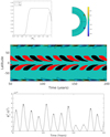 |
Fig. 1. Top panel, left: radial profile of mean-field α-coefficient and the Babcock–Leighton source term due to ephemeral regions. Right: poloidal field line contours obtained from the double-ring algorithm in the northern and southern hemispheres, respectively. Middle panel: butterfly diagram generated from our simulation in the diffusion-dominated region. Bottom panel: typical variation of |

We perform all of our dynamo simulations within the meridional slab 0.55 R⊙ < r < R⊙ and 0 < θ < π with a resolution of 300 × 300 (i.e. Nr = Nθ = 300). We set A = 0 and B ∝ sin(2θ)sin(π((r − 0.55 R⊙)/(R⊙ − 0.55 R⊙))) as dipolar initial conditions for our simulations. Finally, we solve the dynamo equations with proper boundary conditions suitable for the Sun. As our model is axisymmetric, we set both poloidal and toridal fields at zero (A = 0 and B = 0) at the pole (θ = 0 and θ = π) to avoid any kind of singularity. The inner boundary condition at the bottom of the computational domain (r = 0.55 R⊙) is of a perfect conductor. Therefore, at r = 0.55 R⊙, both the toroidal and poloidal field components vanish (i.e. A = 0 and B = 0). We assume that there is only the radial component of the solar magnetic field at the surface, which is necessary for stress balance between the subsurface and coronal magnetic fields (van Ballegooijen & Mackay 2007). We set B = 0 and ∂(rA)/∂r = 0 as a top boundary condition at the surface (r = R⊙).
3. Results
In order to constrain the impact of the mean-field α effect on the memory of the solar cycle, we perform kinematic solar dynamo simulations in two different regimes: advection dominated (ηcz = 1 × 1012 cm2 s−1, v0 = 25 m s−1) and diffusion dominated (ηcz = 1 × 1012 cm2 s−1, v0 = 15 m s−1). Advection-dominated regimes are characterised by the dominance of meridional circulation as a major poloidal flux transport mechanism from the surface to the base of the convection zone, while diffusion-dominated regimes are characterised by the dominance of diffusion (Yeates et al. 2008; Karak & Nandy 2012). We define the advective flux transport timescale following the suggestions of Yeates et al. (2008). The advective flux transport timescale is the time taken for the meridional circulation to transport poloidal fields from r = 0.95 R⊙, θ = 45° to the location at the tachocline where the strongest toroidal field is formed (θ = 60°). The meridional flow speed of the order of 25 m s−1 at the surface yields an advection flux transport timescale of about 9–10 years (with a flow speed of 15 m s−1 this becomes 16 years). While turbulent diffusion of the order of 1 × 1012 cm2 s−1 gives us the diffusion flux transport timescale (L2/η where L is the depth of the convection zone) of 14 years. In the diffusion-dominated regime, the diffusion timescale is shorter than the advection timescale, and vice versa in the advection-dominated regime.
In the first scenario, we consider the Babcock–Leighton mechanism as the only poloidal field generation mechanism. We first perform the simulation without any fluctuation. We are able to reproduce a solar-like cycle with an 11-year periodicity. We also confirm that the periodicity of the solar cycle decreases with the speed of the meridional flow (Dikpati & Charbonneau 1999). Periodicity lies within the range of 7 to 18 years depending on the speed of the meridional flow at the surface, which varies from 25 m s−1 to 10 m s−1. However, in reality, the Babcock–Leighton mechanism is a random process. The stochastic nature of the Babcock–Leighton mechanism arises from the random buffeting of flux tubes during their rise through the turbulent convection zone, yielding a significant scatter in tilt angles of the active region (Longcope & Choudhuri 2002; McClintock & Norton 2016). Motivated by these facts, we introduce stochastic fluctuation in the poloidal field generation source term by setting up K1 = Kbase + Kflucσ(t, τcor) with Kbase = 100 in the double-ring algorithm. Here σ, the uniform random number, lies between −1 and +1. We run all our following simulations with a 60% fluctuation in the Babcock–Leighton mechanism, and therefore in our simulation Kfluc = 0.6Kbase (see Appendix A). Our choice of fluctuation level is inspired by observations as well as the eddy velocity distributions present in 3D turbulent convection simulations (Miesch et al. 2008; Racine et al. 2011; Passos et al. 2012).
The middle panel of Fig. 1 shows the butterfly diagram at the base of the convection zone from a simulation in the diffusion-dominated regime and the bottom panel shows the variation of  (a proxy of sunspot number) with time at the base of the convection zone. We note that the sensitivity of the peak amplitude of the
  is due to the choice of fluctuation level. We calculate the polar radial flux Φr and toroidal flux Φtor using the prescription suggested by Karak & Nandy (2012) and Yeates et al. (2008). The toroidal flux Φtor is calculated by integrating Bϕ(r, θ) within a layer of r = 0.677 R⊙ − 0.726 R⊙ and within the latitude 10 ° −45°; while the radial flux Φr is calculated by integrating Br(R⊙, θ) at the solar surface within the latitude 70 ° −89°. We note that there is a 90° phase difference between the radial flux and the toroidal flux. Radial flux is maximum at the minima of the solar cycle. We find the peak value of Φr and Φtor for each cycle and study the cross-correlation between the surface radial flux Φr of cycle n and the toroidal flux of cycle n, n + 1, n + 2, and n + 3. We perform the same study for both advection-dominated and diffusion-dominated dynamo simulations. Cycle-to-cycle correlation gives us the extent of correlation between the radial and toroidal flux. As per suggestions by Yeates et al. (2008) and Karak & Nandy (2012), the extent of the correlation is an indicator of the memory of the solar cycle. We run our stochastically forced dynamo model for a total of 250 solar cycles to generate the correlation statistics.
Figure 2 shows that in the advection-dominated dynamo, surface radial flux Φr correlates with the toroidal flux Φtor of cycles (n + 1) and (n + 2) with Spearman correlation coefficients 0.90 and 0.49, respectively. On the other hand, Fig. 3 indicates that in the diffusion-dominated dynamo, surface radial flux Φr only correlates with the toroidal flux Φtor of the subsequent cycle (correlation coefficient 0.95). Yeates et al. (2008) studied the memory of the solar cycle and found that in the diffusion-dominated dynamo surface radial flux Φr only correlates with the subsequent cycle toroidal flux Φtor. While, in the advection-dominated dynamo, surface radial flux Φr correlates with the toroidal flux Φtor of subsequent few cycles (n + 1), (n + 2), and (n + 3). Yeates et al. (2008) and Karak & Nandy (2012) found higher correlation coefficients in the advection-dominated regimes than those that we present here. This is probably due to our choice of modelling magnetic buoyancy by the double-ring algorithm. In summary, our results agree with the results of Yeates et al. (2008) when we consider the Babcock–Leighton mechanism as the only poloidal-field-generation process.
 |
Fig. 2. Cross-correlation between the radial flux (Φr) of cycle n and the toroidal flux (Φtor) of cycle n, n + 1, n + 2, n + 3 in the advection-dominated dynamo. The poloidal field is generated only due to the Babcock–Leighton mechanism. Spearman correlation coefficients with significance level are given inside the plots. Here, we consider 60% fluctuations in the Babcock–Leighton mechanism. |
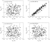 |
Fig. 3. Cross-correlation between the radial flux (Φr) of cycle n and the toroidal flux (Φtor) of cycle n, n + 1, n + 2, n + 3 in the diffusion-dominated dynamo. The poloidal field is generated only due to the Babcock–Leighton mechanism. Spearman correlation coefficients with significance level are given inside the plots. Here, we consider 60% fluctuations in the Babcock–Leighton mechanism. |
In the second scenario, we consider both the Babcock–Leighton mechanism and mean-field α effect as poloidal-field-generation mechanisms. However, the mean-field α effect is also a random process, not a deterministic one. As the mean-field α effect arises due to helical turbulence inside the turbulent convection zone, the mean-field α effect is also a stochastic process. Motivated by these factors, we introduce randomness into the mean-field α by setting S⊙ = Sbase + Sflucσ(t, τcorr). Here, σ is a uniform random number lying between −1 and +1. We set the correlation time τcorr in such a way that at least ten fluctuations are there within a single solar cycle. We run our simulations with a 60% fluctuation in the Babcock–Leighton mechanism and a different level of fluctuation in the mean-field α effect. Figures 4 and 5 show that in the case of both advection- and diffusion-dominated dynamos, surface radial flux Φr only correlates with the toroidal flux of the subsequent cycle with Spearman correlation coefficients of 0.85 and 0.89, respectively. Please note that we use the results of the model with 60% fluctuation in the Babcock–Leighton mechanism and 50% fluctuation in the mean-field α effect to generate Figs. 4 and 5. Tables 1 and 2 summarise results from parameter space studies with variations in the amplitude and fluctuation levels of the mean-field α effect. In our model, the presence of the mean-field α effect reduces the memory of the solar cycle to only one cycle if there is no fluctuation in the mean-field α. However, when fluctuations are introduced in the mean-field α effect, very weak but significant correlations emerge between the radial flux at the nth cycle minima and the toroidal flux at the (n + 2)th cycle maxima for the advection-dominated dynamo (see Table 2). Table 1 shows that the correlation strength between the radial and toroidal flux of various cycles are also dependent on the assumed amplitude of the mean-field α effect (which is restricted to a value of 0.20 m s−1 for reasons of stability). The important conclusion from this study is that we get only one cycle memory even in the case of the advection-dominated convection zone for steady mean-field α (no fluctuations) and that variation in the amplitude or fluctuation levels of mean-field α effect has a small but measurable impact on the memory of the advection-dominated dynamo mechanism.
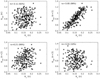 |
Fig. 4. Cross-correlation between the radial flux (Φr) of cycle n and the toroidal flux (Φtor) of cycle n, n + 1, n + 2, n + 3 in the advection-dominated dynamo. The poloidal field is generated due to both the Babcock–Leighton mechanism and mean-field α effect. Spearman correlation coefficients with significance level are given inside the plots. Here, we consider 60% fluctuations in the Babcock–Leighton mechanism and 50% fluctuation in the mean field α. The value of the mean-field α constant factor S⊙ is 0.14. |
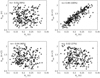 |
Fig. 5. Cross-correlation between the radial flux (Φr) of cycle n and the toroidal flux (Φtor) of cycle n, n + 1, n + 2, n + 3 in the diffusion-dominated dynamo. Poloidal field is generated due to both the Babcock–Leighton mechanism and mean-field α effect. Spearman correlation coefficients with significance level are given inside the plots. Here, we consider 60% fluctuations in the Babcock–Leighton mechanism and 50% fluctuation in the mean field α. The value of the mean-field α constant factor S⊙ is 0.14. |
Correlation coefficients (rs) and percentage significance levels (p) for peak surface radial flux Φr of cycle n versus peak toroidal flux Φtor of different cycles from data for 200 solar cycles.
Correlation coefficients (rs) and percentage significance levels (p) for peak surface radial flux Φr of cycle n versus peak toroidal flux Φtor of different cycles from data for 200 solar cycles.
4. Conclusions
In summary, we demonstrate that inclusion of the mean-field α effect has a measurable impact on the memory of the solar cycle. We find that solar-cycle memory is only limited to one cycle when a basal steady mean-field α effect is included in a flux-transport-type dynamo model and acts in conjunction with the Babcock–Leighton mechanism. This result supports earlier suggestions regarding the precursor value of the poloidal field at the end of a cycle for the amplitude of the subsequent cycle alone (Schatten et al. 1978; Solanki et al. 2002; Yeates et al. 2008; Karak & Nandy 2012; Muñoz-Jaramillo et al. 2013; Sanchez et al. 2014). Our detailed analysis shows that the presence of a mean-field α effect in the dynamo model adds more complexity to the interpretation of differences in the memory of the solar dynamo in the context of advection- versus diffusion-dominated solar convection zones. Specifically, we find that variations in the amplitude or fluctuation levels of the mean-field α can have a weak but measurable impact on the emergence of multi-cycle memory in the advection-dominated solar dynamo.
We do not consider turbulent pumping in our simulations. Karak & Nandy (2012) show that turbulent pumping can impact the memory of the solar cycle. These latter authors found that in the case of both advection- and diffusion-dominated regimes, surface radial flux Φr only correlates with the subsequent cycle toroidal flux if turbulent pumping is added to their model. However, Karak & Nandy (2012) did not include the mean-field α effect in their dynamo simulations. We also find that surface radial flux Φr correlates only with the toroidal flux Φtor of the subsequent cycle when we include turbulent pumping in our simulations with mean-field α effect which extends the validity of the earlier results. It has been argued that the relative efficiency between different flux transport mechanisms governs the memory of the solar cycle. In the model that considers the Babcock–Leighton mechanism as the sole poloidal field generation mechanism, the timescale for transport of the poloidal flux from the surface to the base of the convection zone governs the memory of the solar cycle. Even for a modest radial turbulent pumping speed of 2 m s−1, the timescale for transport of the poloidal flux from surface to the base of the convection zone is only 3.4 years. The introduction of turbulent pumping in the flux transport dynamo model makes the dynamo model completely dominated by turbulent pumping, eventually impacting the memory of the solar cycle. In the situation where turbulent pumping dominates the vertical flux transport mechanism, the relative efficiency of other flux transport mechanisms, namely meridional circulation and turbulent diffusion, is less significant.
In our model, the poloidal field generation takes place due to the combined effect of both the Babcock–Leighton mechanism and the mean-field α effect. As poloidal field generation takes place throughout the convection zone due to the mean-field α effect, the poloidal flux becomes immediately available for being inducted to the toroidal component by the differential rotation. In the absence of any additional complexities, this would normally result in a reduction of the cycle memory to only one cycle – as seen in our case with no fluctuation in mean-field α. However, introduction of fluctuations in the mean-field α effect and variations in the relative strengths of the competing mean-field and Babcock–Leighton poloidal sources may result in a redistribution of the memory across cycles in the advection-dominated regime; we speculate that this is at the origin of the emergence of weak multi-cycle correlations and their variations with increasing levels of fluctuation in the mean-field α effect.
Taken together, we argue that additional consideration of a mean-field α effect within the framework of a flux transport dynamo model – driven by a Babcock–Leighton mechanism – introduces subtleties in the dynamics that may be weak, but may still be important to capture from the perspective of predictive dynamo models. Predictive mode coupled surface flux transport and dynamo simulations support this argument in the context of the successful reconstruction of past solar activity cycles (Bhowmik & Nandy 2018). Completely independent considerations of cycle recovery following a grand minimum in activity also support the importance of a mean-field α effect in the bulk of the solar convection zone – even if it is weak in strength (Hazra et al. 2014a; Passos et al. 2014). We therefore conclude that it may be necessary to include the physics of the mean-field α effect in predictive dynamo models of the solar cycle, even if the Babcock–Leighton mechanism are the dominant source for poloidal field generation.
Acknowledgments
We thank Antoine Strugarek and Eric Buchlin for reading this manuscript and providing useful suggestions. We also thank the anonymous referee for the constructive suggestions which have improved the work further. We thank the Université Paris-Saclay (IRS SPACEOBS grant), ERC Synergy grant 810218 (Whole Sun project), INSU/PNST and CNES Solar Orbiter for supporting this research. The Center of Excellence in Space Sciences India (CESSI) is supported by the Ministry of Human Resource Development, Government of India under the Frontier Areas of Science and Technology (FAST) scheme.
References
- Babcock, H. W. 1961, ApJ, 133, 572 [Google Scholar]
- Bhowmik, P. 2019, A&A, 632, A117 [CrossRef] [EDP Sciences] [Google Scholar]
- Bhowmik, P., & Nandy, D. 2018, Nat. Commun., 9, 5209 [Google Scholar]
- Brun, A. S. 2007, Astron. Nachr., 328, 1137 [NASA ADS] [CrossRef] [Google Scholar]
- Brun, A. S., & Browning, M. K. 2017, Liv. Rev. Sol. Phys., 14, 4 [Google Scholar]
- Brun, A. S., García, R. A., Houdek, G., Nandy, D., & Pinsonneault, M. 2015, Space Sci. Rev., 196, 303 [NASA ADS] [CrossRef] [Google Scholar]
- Cameron, R. H., & Schüssler, M. 2016, A&A, 591, A46 [NASA ADS] [CrossRef] [EDP Sciences] [Google Scholar]
- Charbonneau, P. 2005, Liv. Rev. Sol. Phys., 2, 2 [Google Scholar]
- Choudhuri, A. R., & Karak, B. B. 2012, Phys. Rev. Lett., 109, 171103 [NASA ADS] [CrossRef] [Google Scholar]
- Choudhuri, A. R., Chatterjee, P., & Nandy, D. 2004, ApJ, 615, L57 [NASA ADS] [CrossRef] [Google Scholar]
- Choudhuri, A. R., Chatterjee, P., & Jiang, J. 2007, Phys. Rev. Lett., 98, 131103 [Google Scholar]
- Dikpati, M., & Charbonneau, P. 1999, ApJ, 518, 508 [NASA ADS] [CrossRef] [Google Scholar]
- Dikpati, M., de Toma, G., & Gilman, P. A. 2006, Geophys. Res. Lett., 33, L05102 [NASA ADS] [CrossRef] [Google Scholar]
- Do Cao, O., & Brun, A. S. 2011, Astron. Nachr., 332, 907 [NASA ADS] [CrossRef] [Google Scholar]
- Durney, B. R. 1997, ApJ, 486, 1065 [NASA ADS] [CrossRef] [Google Scholar]
- Fan, Y., Fisher, G. H., & McClymont, A. N. 1994, ApJ, 436, 907 [NASA ADS] [CrossRef] [Google Scholar]
- Hathaway, D. H. 2009, Space Sci. Rev., 144, 401 [NASA ADS] [CrossRef] [Google Scholar]
- Hathaway, D. H., Gilman, P. A., Harvey, J. W., et al. 1996, Science, 272, 1306 [NASA ADS] [CrossRef] [Google Scholar]
- Hazra, G., & Miesch, M. S. 2018, ApJ, 864, 110 [NASA ADS] [CrossRef] [Google Scholar]
- Hazra, S., & Nandy, D. 2013, in Astron. Soc. India Conf. Ser., 10 [Google Scholar]
- Hazra, S., & Nandy, D. 2016, ApJ, 832, 9 [NASA ADS] [CrossRef] [Google Scholar]
- Hazra, S., & Nandy, D. 2019, MNRAS, 489, 4329 [CrossRef] [Google Scholar]
- Hazra, G., Karak, B. B., & Choudhuri, A. R. 2014a, ApJ, 782, 93 [NASA ADS] [CrossRef] [Google Scholar]
- Hazra, S., Passos, D., & Nandy, D. 2014b, ApJ, 789, 5 [NASA ADS] [CrossRef] [Google Scholar]
- Hazra, G., Choudhuri, A. R., & Miesch, M. S. 2017, ApJ, 835, 39 [NASA ADS] [CrossRef] [Google Scholar]
- Hung, C. P., Brun, A. S., Fournier, A., et al. 2017, ApJ, 849, 160 [CrossRef] [Google Scholar]
- Inceoglu, F., Simoniello, R., Arlt, R., & Rempel, M. 2019, A&A, 625, A117 [CrossRef] [EDP Sciences] [Google Scholar]
- Jackiewicz, J., Serebryanskiy, A., & Kholikov, S. 2015, ApJ, 805, 133 [NASA ADS] [CrossRef] [Google Scholar]
- Jouve, L., & Brun, A. S. 2007, A&A, 474, 239 [NASA ADS] [CrossRef] [EDP Sciences] [Google Scholar]
- Jouve, L., Proctor, M. R. E., & Lesur, G. 2010, A&A, 519, A68 [NASA ADS] [CrossRef] [EDP Sciences] [Google Scholar]
- Jouve, L., Brun, A. S., & Talagrand, O. 2011, ApJ, 735, 31 [CrossRef] [Google Scholar]
- Käpylä, P. J., Korpi, M. J., Ossendrijver, M., & Stix, M. 2006a, A&A, 455, 401 [NASA ADS] [CrossRef] [EDP Sciences] [Google Scholar]
- Käpylä, P. J., Korpi, M. J., & Tuominen, I. 2006b, Astron. Nachr., 327, 884 [NASA ADS] [CrossRef] [Google Scholar]
- Karak, B. B., & Miesch, M. 2017, ApJ, 847, 69 [NASA ADS] [CrossRef] [Google Scholar]
- Karak, B. B., & Miesch, M. 2018, ApJ, 860, L26 [Google Scholar]
- Karak, B. B., & Nandy, D. 2012, ApJ, 761, L13 [NASA ADS] [CrossRef] [Google Scholar]
- Komm, R. W., Howard, R. F., & Harvey, J. W. 1993, Sol. Phys., 147, 207 [Google Scholar]
- Komm, R. W., Howard, R. F., & Harvey, J. W. 1995, Sol. Phys., 158, 213 [NASA ADS] [Google Scholar]
- Kumar, R., Jouve, L., & Nandy, D. 2019, A&A, 623, A54 [NASA ADS] [CrossRef] [EDP Sciences] [Google Scholar]
- Leighton, R. B. 1969, ApJ, 156, 1 [Google Scholar]
- Lemerle, A., Charbonneau, P., & Carignan-Dugas, A. 2015, ApJ, 810, 78 [NASA ADS] [CrossRef] [Google Scholar]
- Longcope, D., & Choudhuri, A. R. 2002, Sol. Phys., 205, 63 [NASA ADS] [CrossRef] [Google Scholar]
- Mason, J., Hughes, D. W., & Tobias, S. M. 2008, MNRAS, 391, 467 [CrossRef] [Google Scholar]
- McClintock, B. H., & Norton, A. A. 2016, ApJ, 818, 7 [Google Scholar]
- Miesch, M. S., Brun, A. S., DeRosa, M. L., & Toomre, J. 2008, ApJ, 673, 557 [NASA ADS] [CrossRef] [Google Scholar]
- Miesch, M. S., Featherstone, N. A., Rempel, M., & Trampedach, R. 2012, ApJ, 757, 128 [NASA ADS] [CrossRef] [Google Scholar]
- Moffatt, H. K. 1978, Magnetic Field Generation in Electrically Conducting Fluids [Google Scholar]
- Muñoz-Jaramillo, A., Nandy, D., & Martens, P. C. H. 2009, ApJ, 698, 461 [NASA ADS] [CrossRef] [Google Scholar]
- Muñoz-Jaramillo, A., Nandy, D., Martens, P. C. H., & Yeates, A. R. 2010, ApJ, 720, L20 [CrossRef] [Google Scholar]
- Muñoz-Jaramillo, A., Nandy, D., & Martens, P. C. H. 2011, ApJ, 727, L23 [NASA ADS] [CrossRef] [Google Scholar]
- Muñoz-Jaramillo, A., Dasi-Espuig, M., Balmaceda, L. A., & DeLuca, E. E. 2013, ApJ, 767, L25 [Google Scholar]
- Nandy, D., & Choudhuri, A. R. 2001, ApJ, 551, 576 [NASA ADS] [CrossRef] [Google Scholar]
- Nandy, D., & Choudhuri, A. R. 2002, Science, 296, 1671 [NASA ADS] [CrossRef] [PubMed] [Google Scholar]
- Nandy, D., Muñoz-Jaramillo, A., & Martens, P. C. H. 2011, Nature, 471, 80 [NASA ADS] [CrossRef] [Google Scholar]
- Ossendrijver, M., Stix, M., Brandenburg, A., & Rüdiger, G. 2002, A&A, 394, 735 [NASA ADS] [CrossRef] [EDP Sciences] [Google Scholar]
- Parker, E. N. 1955, ApJ, 121, 491 [NASA ADS] [CrossRef] [Google Scholar]
- Parker, E. N. 1979, Cosmical Magnetic Fields. Their Origin and Their Activity [Google Scholar]
- Passos, D., Charbonneau, P., & Beaudoin, P. 2012, Sol. Phys., 279, 1 [Google Scholar]
- Passos, D., Nandy, D., Hazra, S., & Lopes, I. 2014, A&A, 563, A18 [NASA ADS] [CrossRef] [EDP Sciences] [Google Scholar]
- Pesnell, W. D. 2008, Sol. Phys., 252, 209 [NASA ADS] [CrossRef] [Google Scholar]
- Petrovay, K. 2010, Liv. Rev. Sol. Phys., 7, 6 [Google Scholar]
- Pipin, V. V., & Kosovichev, A. G. 2011, ApJ, 741, 1 [NASA ADS] [CrossRef] [Google Scholar]
- Pipin, V. V., Zhang, H., Sokoloff, D. D., Kuzanyan, K. M., & Gao, Y. 2013, MNRAS, 435, 2581 [CrossRef] [Google Scholar]
- Priest, E. 2014, Magnetohydrodynamics of the Sun [Google Scholar]
- Racine, É., Charbonneau, P., Ghizaru, M., Bouchat, A., & Smolarkiewicz, P. K. 2011, ApJ, 735, 46 [NASA ADS] [CrossRef] [Google Scholar]
- Rajaguru, S. P., & Antia, H. M. 2015, ApJ, 813, 114 [NASA ADS] [CrossRef] [Google Scholar]
- Sanchez, S., Fournier, A., & Aubert, J. 2014, ApJ, 781, 8 [NASA ADS] [CrossRef] [Google Scholar]
- Schatten, K. H., Scherrer, P. H., Svalgaard, L., & Wilcox, J. M. 1978, Geophys. Res. Lett., 5, 411 [NASA ADS] [CrossRef] [Google Scholar]
- Schrijver, C. J., Kauristie, K., Aylward, A. D., et al. 2015, Adv. Space Res., 55, 2745 [Google Scholar]
- Snodgrass, H. B., & Dailey, S. B. 1996, Sol. Phys., 163, 21 [NASA ADS] [CrossRef] [Google Scholar]
- Solanki, S. K., Krivova, N. A., Schüssler, M., & Fligge, M. 2002, A&A, 396, 1029 [NASA ADS] [CrossRef] [EDP Sciences] [Google Scholar]
- Steenbeck, M., Krause, F., & Rädler, K. H. 1966, Z. Naturforsch. Teil A, 21, 369 [CrossRef] [Google Scholar]
- Švanda, M., Brun, A. S., Roudier, T., & Jouve, L. 2016, A&A, 586, A123 [CrossRef] [EDP Sciences] [Google Scholar]
- van Ballegooijen, A. A., & Mackay, D. H. 2007, ApJ, 659, 1713 [NASA ADS] [CrossRef] [Google Scholar]
- Yeates, A. R., & Muñoz-Jaramillo, A. 2013, MNRAS, 436, 3366 [Google Scholar]
- Yeates, A. R., Nandy, D., & Mackay, D. H. 2008, ApJ, 673, 544 [NASA ADS] [CrossRef] [Google Scholar]
- Zhao, J., & Chen, R. 2016, Asian J. Phys., 25, 325 [Google Scholar]
Appendix A: Modelling the Babcock–Leighton mechanism
Poloidal field generation at the surface takes place due to the decay and dispersal of the bipolar sunspot regions as well as ephemeral regions. We model the poloidal field generation mechanism at the surface due to ephemeral regions following an equation similar to Eq. (8):
![Mathematical equation: $$ \begin{aligned}&S_{\rm EPR} = S_{1} \frac{ \cos \theta }{4} \left[1+\mathrm {erf} \left( \frac{r-r_1}{d_1}\right)\right] \left[1-\text{ erf}\left( \frac{r-r_2}{d_2}\right)\right] \nonumber \\&\qquad \quad \times \frac{1}{1+\left(\frac{B_\phi }{B_{\rm up}}\right)^2} , \end{aligned} $$](/articles/aa/full_html/2020/10/aa37287-19/aa37287-19-eq13.gif) (A.1)
(A.1)
where we take r1 = 0.95 R0, r2 = R0, d1 = d2 = 0.15 R0, and Bup = 104 G. Here, S1 controls the amplitude of the poloidal field generation mechanism due to ephemeral regions. We take S1 = 0.13 in our model.
In our model, we follow the prescription of the double-ring algorithm proposed by Durney (1997) to model the active region. In this algorithm, we define the ϕ component of potential vector A associated with the active region as:
 (A.2)
(A.2)
where constant K1 ensures the super-critical dynamo solution and A(Φ) defines the strength of the ring doublet. F(r) is defined as:
![Mathematical equation: $$ \begin{aligned} F(r)= \left\{ \begin{array}{cc} 0&r < R_\odot -R_{ar}\\ \frac{1}{r}\sin ^2\left[\frac{\pi }{2 R_{ar}}(r - (R_\odot -R_{ar}))\right]&r\ge R_\odot -R_{ar} \end{array}\right., \end{aligned} $$](/articles/aa/full_html/2020/10/aa37287-19/aa37287-19-eq15.gif) (A.3)
(A.3)
where R⊙ is the solar radius and the penetration depth of the active region is Rar = 0.85 R⊙. G(θ) in the integral form is defined as:
![Mathematical equation: $$ \begin{aligned} G(\theta ) = \frac{1}{\sin {\theta }}\int _0^{\theta }[B_{-}(\theta ^{\prime })+B_{+}(\theta ^{\prime })]\sin (\theta ^{\prime })\mathrm{d}\theta ^{\prime }, \end{aligned} $$](/articles/aa/full_html/2020/10/aa37287-19/aa37287-19-eq16.gif) (A.4)
(A.4)
where B+ (B−) represents the strength of positive (negative) ring:
![Mathematical equation: $$ \begin{aligned} B_{\pm }(\theta )= \left\{ \begin{array}{cc} 0&\theta <\theta _{ar}\mp \frac{\chi }{2}-\frac{\Lambda }{2}\\ \pm \frac{1}{\sin (\theta )}\left[1+\cos \left(\frac{2\pi }{\Lambda }(\theta -\theta _{ar}\pm \frac{\chi }{2})\right)\right] \\ \theta _{ar}\mp \frac{\chi }{2}-\frac{\Lambda }{2} \le \theta < \theta _{ar}\mp \frac{\chi }{2}+\frac{\Lambda }{2}\\ 0&\theta \ge \theta _{ar}\mp \frac{\chi }{2}+\frac{\Lambda }{2}, \end{array}\right. \end{aligned} $$](/articles/aa/full_html/2020/10/aa37287-19/aa37287-19-eq17.gif) (A.5)
(A.5)
where θar is the colatitude of the double ring emergence and the diameter of each polarity of the double ring is Λ. We take the latitudinal distance between the centres of the double ring as χ = arcsin[sin(β) sin(Δar)], where Δar is the angular distance between polarity centres and β is the active region tilt angle. We take Λ and Δar as 6° for our model.
Regenerating the poloidal field. To recreate the poloidal field at the solar surface, we first randomly choose a latitude from both the hemispheres where the toroidal field exceeds the buoyancy threshold at the bottom of the convection zone. We then use a non-uniform probability distribution function to ensure that randomly chosen latitude always remains within the observed active region belt. Next, we calculate the tilt of the corresponding active region following the expression prescribed in Fan et al. (1994):
 (A.6)
(A.6)
where, Φ0 is the toroidal ring associated flux, B0 is the local field strength, and λ is the chosen latitude for the ring emergence. The constant that appears in Eq. (A.6) is fixed in a way such that the tilt angle lies between 3° and 12°. Next, we remove a part of the magnetic field with the same angular size of the emerging active region from this toroidal ring. We reduced the magnetic field strength of the toroidal ring from which the active region erupts. We set the toroidal field strength in such a way that the energy of the full toroidal ring with the new magnetic field is equal to the energy of the partial toroidal ring with the old magnetic field (after removing a chunk of the magnetic field). Finally, we place the ring doublets with these calculated properties at the near-surface layer at the chosen erupted latitude. Figure 1 (right side-top panel) shows the poloidal field line contours associated with the double ring in both hemispheres for one particular time-step.
All Tables
Correlation coefficients (rs) and percentage significance levels (p) for peak surface radial flux Φr of cycle n versus peak toroidal flux Φtor of different cycles from data for 200 solar cycles.
Correlation coefficients (rs) and percentage significance levels (p) for peak surface radial flux Φr of cycle n versus peak toroidal flux Φtor of different cycles from data for 200 solar cycles.
All Figures
|
Fig. 1. Top panel, left: radial profile of mean-field α-coefficient and the Babcock–Leighton source term due to ephemeral regions. Right: poloidal field line contours obtained from the double-ring algorithm in the northern and southern hemispheres, respectively. Middle panel: butterfly diagram generated from our simulation in the diffusion-dominated region. Bottom panel: typical variation of |
| In the text | |
|
Fig. 2. Cross-correlation between the radial flux (Φr) of cycle n and the toroidal flux (Φtor) of cycle n, n + 1, n + 2, n + 3 in the advection-dominated dynamo. The poloidal field is generated only due to the Babcock–Leighton mechanism. Spearman correlation coefficients with significance level are given inside the plots. Here, we consider 60% fluctuations in the Babcock–Leighton mechanism. |
| In the text | |
|
Fig. 3. Cross-correlation between the radial flux (Φr) of cycle n and the toroidal flux (Φtor) of cycle n, n + 1, n + 2, n + 3 in the diffusion-dominated dynamo. The poloidal field is generated only due to the Babcock–Leighton mechanism. Spearman correlation coefficients with significance level are given inside the plots. Here, we consider 60% fluctuations in the Babcock–Leighton mechanism. |
| In the text | |
|
Fig. 4. Cross-correlation between the radial flux (Φr) of cycle n and the toroidal flux (Φtor) of cycle n, n + 1, n + 2, n + 3 in the advection-dominated dynamo. The poloidal field is generated due to both the Babcock–Leighton mechanism and mean-field α effect. Spearman correlation coefficients with significance level are given inside the plots. Here, we consider 60% fluctuations in the Babcock–Leighton mechanism and 50% fluctuation in the mean field α. The value of the mean-field α constant factor S⊙ is 0.14. |
| In the text | |
|
Fig. 5. Cross-correlation between the radial flux (Φr) of cycle n and the toroidal flux (Φtor) of cycle n, n + 1, n + 2, n + 3 in the diffusion-dominated dynamo. Poloidal field is generated due to both the Babcock–Leighton mechanism and mean-field α effect. Spearman correlation coefficients with significance level are given inside the plots. Here, we consider 60% fluctuations in the Babcock–Leighton mechanism and 50% fluctuation in the mean field α. The value of the mean-field α constant factor S⊙ is 0.14. |
| In the text | |
Current usage metrics show cumulative count of Article Views (full-text article views including HTML views, PDF and ePub downloads, according to the available data) and Abstracts Views on Vision4Press platform.
Data correspond to usage on the plateform after 2015. The current usage metrics is available 48-96 hours after online publication and is updated daily on week days.
Initial download of the metrics may take a while.