| Issue |
A&A
Volume 620, December 2018
|
|
|---|---|---|
| Article Number | A171 | |
| Number of page(s) | 12 | |
| Section | Planets and planetary systems | |
| DOI | https://doi.org/10.1051/0004-6361/201833423 | |
| Published online | 14 December 2018 | |
The CARMENES search for exoplanets around M dwarfs
The warm super-Earths in twin orbits around the mid-type M dwarfs Ross 1020 (GJ 3779) and LP 819-052 (GJ 1265)★
1
Instituto de Astrofísica de Canarias,
38205
La Laguna,
Tenerife,
Spain
e-mail: This email address is being protected from spambots. You need JavaScript enabled to view it.
2
Departamento de Astrofísica, Universidad de La Laguna,
38206
La Laguna,
Tenerife,
Spain
3
Max-Planck-Institut für Astronomie,
Königstuhl 17,
69117
Heidelberg,
Germany
4
Institut für Astrophysik, Georg-August-Universität,
Friedrich-Hund-Platz 1,
37077
Göttingen,
Germany
5
Institut de Ciències de l’Espai (ICE, CSIC), Campus UAB,
c/ de Can Magrans s/n,
08193
Bellaterra,
Barcelona,
Spain
6
Institut d’Estudis Espacials de Catalunya (IEEC),
08034
Barcelona,
Spain
7
Centro de Astrobiología (CSIC-INTA), ESAC Campus, Camino Bajo del Castillo s/n,
28692
Villanueva de la Cañada,
Madrid,
Spain
8
Instituto de Astrofísica de Andalucía (IAA-CSIC), Glorieta de la Astronomía s/n,
18008
Granada,
Spain
9
Landessternwarte, Zentrum für Astronomie der Universtät Heidelberg,
Königstuhl 12,
69117
Heidelberg,
Germany
10
Centro Astronómico Hispano-Alemán (CSIC-MPG), Observatorio Astronómico de Calar Alto, Sierra de los Filabres,
04550
Gérgal,
Almería,
Spain
11
Departamento de Astrofísica y Ciencias de la Atmósfera, Facultad de Ciencias Físicas, Universidad Complutense de Madrid,
28040
Madrid,
Spain
12
Thüringer Landessternwarte Tautenburg,
Sternwarte 5,
07778
Tautenburg,
Germany
13
Hamburger Sternwarte,
Gojenbergsweg 112,
21029
Hamburg,
Germany
14
School of Geosciences, Raymond and Beverly Sackler Faculty of Exact Sciences, Tel Aviv University,
Tel Aviv 6997801,
Israel
Received:
14
May
2018
Accepted:
16
October
2018
Abstract
We announce the discovery of two planetary companions orbiting around the low-mass stars Ross 1020 (GJ 3779, M4.0V) and LP 819-052 (GJ 1265, M4.5V). The discovery is based on the analysis of CARMENES radial velocity (RV) observations in the visual channel as part of its survey for exoplanets around M dwarfs. In the case of GJ 1265, CARMENES observations were complemented with publicly available Doppler measurements from HARPS. The datasets reveal two planetary companions, one for each star, that share very similar properties: minimum masses of 8.0 ± 0.5 M⊕ and 7.4 ± 0.5 M⊕ in low-eccentricity orbits with periods of 3.023 ± 0.001 d and 3.651 ± 0.001 d for GJ 3779 b and GJ 1265 b, respectively. The periodic signals around 3 d found in the RV data have no counterpart in any spectral activity indicator. Furthermore, we collected available photometric data for the two host stars, which confirm that the additional Doppler variations found at periods of approximately 95 d can be attributed to the rotation of the stars. The addition of these planets to a mass-period diagram of known planets around M dwarfs suggests a bimodal distribution with a lack of short-period low-mass planets in the range of 2–5 M⊕. It also indicates that super-Earths (>5 M⊕) currently detected by RV and transit techniques around M stars are usually found in systems dominated by a single planet.
Key words: techniques: radial velocities / stars: late-type / stars: low-mass / planetary systems
The RV and formal uncertainties of GJ 3779 and GJ 1265 are only available at the CDS via anonymous ftp to cdsarc.u-strasbg.fr (130.79.128.5) or via http://cdsarc.u-strasbg.fr/viz-bin/qcat?J/A+A/620/A171
© ESO 2018
1 Introduction
The search for exoplanets has become a prominent research field in the past twenty years, particularly the detection of rocky planets in the habitable zones of their parent stars. The radial velocity (RV) technique has been successfully applied to detect such companions around M dwarfs given the relatively low mass of these stars (Marcy et al. 1998; Rivera et al. 2005; Udry et al. 2007; Bonfils et al. 2013; Anglada-Escudé et al. 2016). M stars account for three quarters of all stars known within 10 pc of our solar system (Henry et al. 2016) and show an average occurrence rate of more than two planets per host star (Dressing & Charbonneau 2015; Gaidos et al. 2016).
Despite their high potential for finding rocky planets, M dwarfs pose various observational difficulties. On the one hand, low-mass stars emit more flux in the near-infrared (NIR) than in the visual (VIS). On the other hand, chromospheric variability and activity cycles may produce changes in the spectral line profiles, which mimic a Doppler shift. These periodic variations induce signals in the RV data that could be incorrectly interpreted as being of planetary origin (e.g. Queloz et al. 2001; Robertson et al. 2014; Sarkis et al. 2018). Since stellar jitter can reach amplitudes of a few metres per second, detecting low-signal companions generally requires a considerable number of observations (Barnes et al. 2011). However, since the amplitude of an activity-related signal is expected to be wavelength-dependent, a successful program searching for exoplanets around M dwarfs must tackle these difficulties by observing simultaneously in the widest possible wavelength range, especially covering the reddest optical wavelengths, and following an observing strategy that ensures numerous and steady observations covering a long time span.
The CARMENES search for exoplanets around M dwarfs accomplishes these requirements in its guaranteed time observation (GTO) M dwarf survey, which began in January 2016 (Reiners et al. 2018b). Ross 1020 (GJ 3779) and LP 819-052 (GJ 1265) are two mid-type M dwarfs monitored as part of this project. Their RVs indicate the presence of two super-Earths in short-period orbits of theorder of 3 d. Section 2 summarises the basic information of the host stars. In Sect. 3, the RV observations for each star are presented. The analysis of the RV data is explained in Sect. 4, while in Sect. 5 we discuss the results from the Keplerian fit and the location of the two planets in a mass-period diagram.
2 Stellar parameters
The basic information of the host stars GJ 3779 and GJ 1265 is presented in Table 1. Both targets exhibit similar properties and their values are consistent with the literature. They are mid-type M dwarfs that kinematically belong to the Galactic thin disc (Cortés-Contreras 2016), with GJ 1265 being part of the young population. Their photospheric metallicities are compatible with solar values (Neves et al. 2014; Newton et al. 2014; Passegger et al. 2018). They are thought to be inactive, with no emission in Hα (Jeffers et al. 2018) and only very faint X-ray emission for the case of GJ 1265 (Rosen et al. 2016). The photospheric parameters of the stars were determined as in Passegger et al. (2018) using the latest grid of PHOENIX-ACES model spectra (Husser et al. 2013) and the method described in Passegger et al. (2016). We determined the radii R using Stefan–Boltzmann’s law, the spectroscopic Teff as in Passegger et al. (2018), and the luminosities L by integrating the photometric stellar energy distribution collected for the CARMENES targets (Caballero et al. 2016) with the Virtual Observatory Spectral energy distribution Analyser (Bayo et al. 2008). The stellar masses were derived from the linear M–R relation presented by Schweitzer et al. (in prep.). These values are the same using instead empirical mass–luminosity relations such as those presented by Delfosse et al. (2000) and Benedict et al. (2016). The details of the calculation of the physical parameters are described in Reiners et al. (2018a) and will be reported in further detail by Schweitzer et al. (in prep.).
The star GJ 3779 (Ross 1020, J13229+244) is a high proper motion star classified as M4.0 V by Hawley et al. (1996). It resides in the Coma Berenices constellation, located at a distance of d = 13.748 ± 0.011 pc (Gaia Collaboration 2018) with an apparent magnitude in the J band of 8.728 mag (Skrutskie et al. 2006). Using CARMENES data, Reiners et al. (2018b) determined its absolute RV to be Vr =−19.361 km s-1 and a Doppler broadening upper-limit of vsini < 2 km s-1.
The object GJ 1265 (LP 819-052, J22137-176) is also a high proper motion star at a distance of d = 10.255 ± 0.007 pc (Gaia Collaboration 2018) in the Aquarius constellation. Its apparent magnitude in the J band is 8.955 mag (Skrutskie et al. 2006), and it is approaching the solar system with an absolute RV of Vr = −24.297 km s-1 (Reiners et al. 2018b). The star exhibits a luminosity in X-rays of logLX = 26.1 ± 0.2 erg s-1, measured with the XMM-Newton observatory (Rosen et al. 2016). Therefore, we can estimate the rotational period of the star to be of the order of 100 d following the LX –Prot relation proposed by Reiners et al. (2014).
Stellar parameters for GJ 3779 and GJ 1265.
3 Observations
The CARMENES instrument, installed at the 3.5 m Calar Alto telescope at the Calar Alto Observatory in Spain consists of a simultaneous dual-channel fibre-fed high-resolution spectrograph covering a wide wavelength range from 0.52 μm to 0.96 μm in the VIS and from 0.96 μm to 1.71 μm in the NIR, with spectral resolutions of R = 94 600 and R = 80 400, respectively (Quirrenbach et al. 2014). The performance of the instrument and its ability to discover exoplanets around M dwarfs using the RV technique has already been demonstrated by Trifonov et al. (2018), Reiners et al. (2018a), and Kaminski et al. (2018).
The survey contains 104 observations for GJ 3779 in the VIS channel covering a time span of 820 d, with typical exposure times of 1800 s and median internal RV precision of σVIS = 1.7 m s-1. In the case of GJ 1265, 87 observations were acquired in the visible, covering a timespan of 782 d, typical exposure times of 1800 s, and median internal RV precision of σVIS = 1.8 m s-1. The NIR median internal RV precisions are considerably higher: σNIR = 10.4 m s-1 and σNIR = 6.7 m s-1 for GJ 3779 and GJ 1265, respectively. As a result, we only use the RVs from the VIS channel in our analysis.
Doppler measurements, together with several spectral indicators useful to discuss the planetary hypothesis, were obtained with the SERVAL program (Zechmeister et al. 2018) using high signal-to-noise-ratio (S/N) templates created by co-adding all available spectra of each star. They are corrected for barycentric motion (Wright & Eastman 2014) as well as for secular acceleration, which is important for stars with high proper motions (Zechmeister et al. 2009). In addition, the RVs were corrected by means of an instrumental nightly zero-point (NZP), which was calculated from a subset of RV-quiet stars observed each night whose RV standard deviation is less than 10 m s-1. This correction is described in Trifonov et al. (2018). For each spectrum, we also computed the cross-correlation function (CCF) using a weighted mask by co-adding the stellar observations themselves. Fitting a Gaussian function to the final CCF, we determined the RV, FWHM, contrast, and bisector velocity span. The methodology regarding how the CCF is computed for our CARMENES spectra is described in Reiners et al. (2018a).
Moreover, for our southern target, GJ 1265, we further included 11 publicly available observations from HARPS (Mayor et al. 2003)taken between July 2003 and July 2014. We used SERVAL to derive their RVs and obtained a median internal uncertainty of σHARPS = 5.6 m s-1. The individual RVs for GJ 3779 and GJ 1265 are shown in Figs. 3 and 6, respectively.
In addition to the Doppler measurements, we also collected available photometry for both targets with the goal of determining the rotational period. We analysed photometric time series for GJ 3779 from The MEarth Project (Charbonneau et al. 2008; Berta et al. 2012) from January 2009 to July 2010 in the RG715 filter. For GJ 1265 (EPIC 205913009) we employed photometric time series from the K2 space mission during its Campaign 3 (Vanderburg & Johnson 2014) from November 2014 to February 2015. Figure 1 shows the photometricvariability of GJ 1265. Assuming that the signal is close to sinusoidal we derive a rotational period of ~95 d, which agrees with the ~100 d rotational period estimated from the X-ray luminosity presented in Sect. 2. However, due to the mix of periodic and stochastic behaviour of stellar variability and the fact that the K2 time span does not cover a full phase ofsuch a period, we can only conclude that GJ 1265 is a slowly rotating star with a period longer than 70 d.
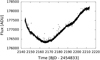 |
Fig. 1 K2 light curve of GJ 1265. The photometric variability of the star is longer than the 69 d baseline of the observations. |
4 Data analysis
4.1 GJ 3779 b
In Fig. 2, we show the generalized Lomb–Scargle periodograms (GLS; Zechmeister & Kürster 2009) of different data products obtained with SERVAL and our CCF analysis. For each panel, we compute the theoretical false alarm probability (FAP) as described in Zechmeister & Kürster (2009), and show the 10%, 1%, and 0.1% levels. In the CARMENES RVs (Fig. 2a), a single relevant peak with FAP = 2.2 × 10⁻³⁵ at f = 0.3307 d-1 (P =3.023 d) is found. The next highest peak in the RVs GLS, though above FAP = 10%, is found at f = 0.0105 d-1 (P =95.24 d), which agrees with the periodic photometric variation found in the MEarth data (Fig. 2c). After subtraction of the 3.023 d periodic signal in the RV GLS, no further significant signals are found (Fig. 2b).
A strong alias1 of the signal discussed so far is found at a frequency of 1 d-1 − f = 0.6693 d-1. A periodogram of the data does not provide information about which of the two peaks is the true planetary signal. However, the peak at 1 d-1 − f, that is, P = 1.494 d, has less power and therefore appears less likely to be the true period. If the fitted signal is the one at P = 1.494 d, the 3.023 d peak in the RV GLS does not disappear, proving that the P = 1.494 d signal is indeed an alias of the ~3 d one. Furthermore, if we choose the true Keplerian period to be the shortest one at ~ 1.5 d, the goodness of the fit gets significantly worse, changing from  to
to  , and the derived eccentricity of the orbit becomes larger, which is unlikely compared to the period and eccentricity distributions of known exoplanets.
Taking full advantage of the spectral information provided by SERVAL and the one contained in the CCF, we further investigate possible periodic signals related with chromospheric activity of the host star that may have induced RV variations. Periodograms of the chromatic index (CRX), differential line width (dLW), and Hα index as described in Zechmeister et al. (2018) are shown in panels d–f of Fig. 2, while full width half maximum (FWHM), contrast (CTR), and bisector velocity span (BVS) from the CCF are shown in panels g–i.
Only the dLW GLS shows significant peaks between 80 and 100 d, almost coincident with those found in the photometry, the radial velocities, best-fit residuals, and the CCF FWHM. We also investigated the nature of the marginal power close to ~ 3 d with FAP ~ 10% present in Fig. 2d. A significant signal in the CRX at the RV period may indicate that the measured Doppler shifts are dependent on wavelength, which would refute the planetary hypothesis. However, we checked that there is no correlation in the RV–CRX scatter plot that may call into question the nature of the periodic signal at f = 0.3307 d-1 (see left panel of Fig. B.1). None of the other indicators show periodicity at this frequency and therefore we conclude that the periodic signal at 3.023 d is due to a planetary origin and the signal at P ~ 95 d is related to the rotation of the star.
To obtain the orbital parameters of the planet, we fit the RV dataset searching for the χ 2 minimum using the Levenberg–Marquardt method (Press et al. 1992) in a Keplerian scheme. The best-fit Keplerian orbital parameters and their corresponding 1σ uncertainties of the planet GJ 3779 b are listed in Table 2. We estimated the uncertainties of the best-fit parameters using two different approaches. First, we obtained the errors given by the covariance matrix in the Levenberg–Marquardt algorithm itself. Second, using the Markov chain Monte Carlo (MCMC) sampler emcee (Foreman-Mackey et al. 2013) and a Keplerian model with flat priors, we can derive median and 1σ uncertainty values from the posterior distributions. A noise term ("jitter") is modelled simultaneously during the parameter optimisation following Baluev (2009). The posterior distributions from the MCMC analysis are shown in Fig. C.1.
The phased RVs and their residuals around the best fit are shown in Fig. 3. The abscissa values of phase-folded plot are determined by computing the difference between each Julian date and the epoch of the first RV observation, and then computing the remainder of the quotient of this difference with the orbital period. The planet candidate GJ 3779 b has a minimum mass of 8.0 ± 0.5 M⊕ orbiting at a semi-major axis of 0.026 au, much closer to the host star than the conservative habitable-zone limits (0.094–0.184au; Kopparapu et al. 2013, 2014). The results from best-fit and MCMC analyses all agree within the uncertainties. The posterior distributions show Gaussian profiles and peak close to the best-fit values from Table 2.
Finally, using the photometric time-series data, we looked for the possibility that GJ 3779 b transits its host star. After detrending and flattening, no significant peaks were found in the box-fitting least squares (BLS) periodogram (Kovács et al. 2002). Nevertheless, we shifted the observations to the predicted secondary transit following Kane et al. (2009) and phase-folded the light curve to the 3.023 d period of the planet. We did not find any hints of transits, as shown in Fig. 4. However, since the radius of the planet could be between 1–3 R⊕ depending on the volatile content, the depth of a hypothetical transit could be between 0.1 and 1.0%. In addition, since the expected duration of the transit is approximately 1 h, the uncertainties of the transit window are large, and there are gaps in the phase-foldedphotometric data, there could still be a chance that the transit was missed or hidden in the noise of the MEarth data. Therefore, we conclude that more data would be required to completely rule out the possibility that GJ 3779 b transits its host star.
Keplerian orbital parameters and 1σ uncertainties of the planet candidates.
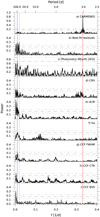 |
Fig. 2 GLS periodograms for GJ 3779 CARMENES RVs (panel a) and its residuals (panel b) after removing the prominent peak at f = 0.3307 d-1 (P = 3.023 d), marked in red. Panel c: periodogram of a photometric campaign of MEarth data from 2010. The highest peak at frot = 0.0105 d-1 (P = 95.2 d) associatedwith the star’s rotation is marked with a solid blue line and its first harmonic (2frot) with a dashed blue line. Panels d–f: periodograms of the chromatic index, differential line width, and Hα index, while panels g–i show periodograms for the cross-correlation function FWHM, contrast, and bisector velocity span. Horizontal lines show the theoretical FAP levels of 10%(short-dashed line), 1% (long-dashed line), and 0.1% (dot-dashed line) for each panel. |
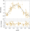 |
Fig. 3 CARMENES RVs and residuals phase-folded to the best Keplerian fitconsistent with a 3.023 d period planet around GJ 3779. |
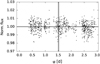 |
Fig. 4 Phase-folded light curve to the 3.023 d planet period of the MEarth photometric data for GJ 3779. The grey shaded area marks the expected transit duration. The central time of the expected transit is also marked with a vertical bar. |
4.2 GJ 1265 b
The same approach as for the previous system was applied for the RV analysis of GJ 1265. The first three panels of Fig. 5 show the GLS periodograms for the CARMENES, HARPS, and combined (CARMENES+HARPS) radial velocities. A prominent single peak at f = 0.2739 d-1 (P = 3.651 d) and its corresponding alias at 1 d-1 − f (Fig. A.1, right panel) can be seen in the CARMENES dataset. Even though the HARPS measurements are not sufficient and are too spread in time to detect the short-period signal in the GLS, when combined with the CARMENES radial velocities the aforementioned peak increases in significance from FAP = 2.1 × 10⁻²⁹ using only CARMENES data to FAP = 1.7 × 10⁻³² adding the HARPS RVs, also improving the frequency resolution. The nature of the peak at 1 d-1 − f has been analysed in the same way as in Sect. 4.1, concluding that it is an alias of the true Keplerian signal. Fitting a sinusoid at 3.651 d, the GLS of the residuals (Fig. 5d) exhibits some power at f <0.012 d-1 (P > 83.3 d), which is compatible with the stellar variability seen in the K2 photometry (Fig. 1) and the predicted rotational period derived in Sect. 2.
In the periodogram analysis of the activity indicators, no remarkable peaks have been found at the frequency of the RV signal or the rotational period of the star. However, following the procedure explained in Sect. 4.1, we checked the nature of the power at ~5 d in the CRX. As in the previous case, no significant correlation was found between the RVs and the CRX in the CARMENES VIS data (Fig. B.1, right panel), either between HARPS RVs and the CCF parameters or Hα. Gathering all the evidence, we conclude that the periodic signal found in the CARMENES RVs can only be due to the star’s reflex motion caused by a planetary companion. Therefore, we took the RVs GLS periodogram peak as initial period guess to fit a Keplerian orbit to the combined RV dataset using the Levenberg–Marquardt method. The best-fit Keplerian orbital parameters and 1σ uncertainties of the planet candidate GJ 1265 b are listed in Table 2, with their corresponding MCMC analysis as explainedin Sect. 4.1 shown in Fig. C.2.
Combined phase-folded RVs together with their best-fit are depicted in Fig. 6. The rms around the best-fit is of 3.0 m s-1 and 8.3 m s-1 for the CARMENES and HARPS RVs, respectively, which corresponds to 1.5σ and 1.2σ given their internal RV uncertainties. The planet orbiting around the M dwarf star GJ 1265 shows similar properties to the one presented in Sect. 4.1, with a minimum mass of 7.4 ± 0.5 M⊕ in a 3.651 d low-eccentricity orbit at a semi-major axis of 0.026 au. The MCMC analysis agrees with the best-fit results within the errors.
As mentioned in Sect. 3, GJ 1265 was observed by the K2 space mission during its Campaign 3. Using this photometry information, we analysed the light curve to look not only for periodic signals associated with the rotation of the star, but also for planetary transits. After removing the photometric variation caused by the rotation of the star, no further signals were found in the BLS periodogram. Nonetheless, we phase-folded the photometric data to the RV signal at 3.651 d to look for possible transits but found none at the period of the planet, as shown in Fig. 7.
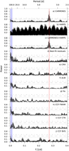 |
Fig. 5 GLS periodograms for GJ 1265 CARMENES (panel a), HARPS (panel b), and combined CARMENES+HARPS (panel c) data. Panel d: residuals after removing the prominent peak at f = 0.2739 d-1 (P = 3.651 d) marked in red. The blue shaded area depicts the excluded planetary region due to stellar variability as discussed in Sect. 3. Panels e–j and horizontal lines are the same as in Fig. 2. |
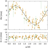 |
Fig. 6 CARMENES (orange) and HARPS (green) radial velocities and residuals phase-folded to the best Keplerian fit consistent with a planet around GJ 1265 with a period of 3.651 d. |
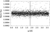 |
Fig. 7 Phase-folded light curve to the 3.651 d planet period of the K2 photometric data for GJ 1265. The grey shaded area marks the expected transit duration. The central time of the expected transit is also marked with a vertical bar. |
5 Discussion and summary
The results from the RV analysis reveal two very similar planets orbiting very similar M dwarfs. Not only do the stars exhibit comparable photospheric and physical parameters but they also show long rotational periods. Mid-type slow-rotators are considered to be less magnetically active than their late-type or rapid-rotator counterparts (West et al. 2015), which agrees with the absence of periodic signals in the photospheric spectral indicators (Figs. 2 and 5). The planetary candidates are both orbiting at a semi-major axes of 0.026 au with periods of the order of 3 d and super-Earth-like minimum masses of 7–8 M⊕. The MCMCanalyses reveal that the derived eccentricities of GJ 3779 b and GJ 1265 b are compatible with circular orbits, which is predicted by orbital evolution models for such short-period planets.
Mass determination for Earth-size and super-Earth planets around M dwarfs is very challenging, and there is a limited number of systems similar to the ones presented here. Only 18 planetary systems have masses derived from RV measurements: GJ 54.1 (Astudillo-Defru et al. 2017b), GJ 1132 (Berta-Thompson et al. 2015), GJ 1214 (Charbonneau et al. 2009), GJ 176 (Forveille et al. 2009), GJ 273 (Astudillo-Defru et al. 2017a), GJ 3138 (Astudillo-Defru et al. 2017a), GJ 3323 (Astudillo-Defru et al. 2017a), GJ 3634 (Bonfils et al. 2011), GJ 3942 (Perger et al. 2017), GJ 3998 (Affer et al. 2016), GJ 433 (Bonfils et al. 2013), GJ 447 (Bonfils et al. 2018), GJ 536 (Suárez Mascareño et al. 2017), GJ 581 (Bonfils et al. 2005), GJ 628 (Wright et al. 2016), GJ 676 A (Anglada-Escudé & Tuomi 2012), GJ 667 C (Bonfils et al. 2013), and GJ 876 (Rivera et al. 2005). Furthermore, the TRAPPIST-1 system was detected by transit search and the planet’s dynamical masses have been inferred from transit timing variations (Gillon et al. 2017; Grimm et al. 2018).
Figure 8 shows the mass-period parameter space of all known M dwarf planets for which both parameters are well-determined. The left panel shows the planets orbiting mid- and late-type M stars, while the right panel also includes those around early-type M dwarfs. The diagrams exhibit a bimodal distribution that resembles the one found in planetary radius using Kepler data mainly for solar-like stars (Fulton et al. 2017; Fulton & Petigura 2018) but also confirmed for validated and well-characterised transiting planets around M dwarfs (Hirano et al. 2018).
We also note the fact that short-period Earth-like planets in the range of 0.5–2 M⊕ are mostly found in multiple systems (triangle symbols), while regarding those in the range of 5–8 M⊕, eight out of ten planets were not found to have further planetary companions. Also striking is the lack of planets in the range of 2–5 M⊕ with orbital periods shorter than 10 d around mid- and late-type M stars. This raises questions about their formation process. Is it possible that super-Earth planets around M dwarfs prevent the formation of smaller counterparts, or are they formed by aggregation of smaller, Earth-size planets? Is the formation of a smaller counterpart dependent on the mass of the host star?
The sample of known planets with accurate mass and radius determinations around M dwarfs is still too small to address the validity of such a distribution, and its connection with planet multiplicity, with any statistical confidence. Ground-based searches, such as the CARMENES GTO program among others, together with planet detections around M dwarfs over the next few years from TESS (Ricker et al. 2014), may provide insight into this issue.
In summary, we report on the discovery of two short-period super-Earth-like planets orbiting the low-mass stars GJ 3779 and GJ 1265. They are the least massive planets discovered by the CARMENES search for exoplanets around M dwarfs to date. The CARMENES visible Doppler measurements reveal a planetary companion with a minimum mass of 8.0 M⊕ on a 3.023 d orbit around GJ 3779, and a planet of 7.4 M⊕ on a 3.651 d orbit around GJ 1265. Besides the periodic signals at around 95 d associated with rotation, the host stars do not show any evidence of RV-induced variations due to activity at the planet periods. The planets do not transit their parent stars, and they seem to belong to a population of short-period single planets around M stars with masses between 5 and 8 M⊕.
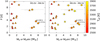 |
Fig. 8 Mass-period diagram of all super-Earth planets, with masses determined from RVs or TTVs, orbiting mid- and late-type M dwarfs (left panel) and for all M dwarfs (right panel) taken from the NASA Exoplanet Archive from May 2018 (https://exoplanetarchive.ipac.caltech.edu). Single- and multi-planet systems are drawn with circles and triangles, respectively.The colorbar indicates the effective temperature of the host star. |
Acknowledgements
CARMENES is an instrument for the Centro Astronómico Hispano-Alemán de Calar Alto (CAHA, Almería, Spain). CARMENES is funded by the German Max-Planck-Gesellschaft (MPG), the Spanish Consejo Superior de Investigaciones Científicas (CSIC), the European Union through FEDER/ERF FICTS-2011-02 funds, and the members of the CARMENES Consortium (Max-Planck-Institut für Astronomie, Instituto de Astrofísica de Andalucía, Landessternwarte Königstuhl, Institut de Ciències de l’Espai, Insitut für Astrophysik Göttingen, Universidad Complutense de Madrid, Thüringer Landessternwarte Tautenburg, Instituto de Astrofísica de Canarias, Hamburger Sternwarte, Centro de Astrobiología and Centro Astronómico Hispano-Alemán), with additional contributions by the Spanish Ministry of Economy, the German Science Foundation through the Major Research Instrumentation Programme and DFG Research Unit FOR2544 “Blue Planets around Red Stars”, the Klaus Tschira Stiftung, the states of Baden-Württemberg and Niedersachsen, and by the Junta de Andalucía. Based on observations collected at the European Organisation for Astronomical Research in the Southern Hemisphere under ESO programme(s) 072.C-0488(E) and 183.C-0437(A). R. L. has received funding from the European Union’s Horizon 2020 research and innovation program under the Marie Skłodowska-Curie grant agreement No. 713673 and financial support through the “la Caixa” INPhINIT Fellowship Grant for Doctoral studies at Spanish Research Centres of Excellence, “la Caixa” Banking Foundation, Barcelona, Spain. This work is partly financed by the Spanish Ministry of Economy and Competitiveness through grants ESP2013-48391-C4-2-R, ESP2016-80435-C2-1/2-R, and AYA2016-79425–C3–1/2/3–P.
Appendix A Frequency-extended periodogram analysis
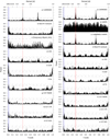 |
Fig. A.1 Extended GLS periodograms for GJ 3779 (left panels) and GJ 1265 (right panels) covering the full frequency range. The magnitudes and the format represented are the same as in Figs. 2 and 5. |
Appendix B Correlation between radial velocities and chromatic index
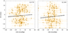 |
Fig. B.1 CARMENES VIS radial velocities against the chromatic index (CRX) for GJ 3779 (left panel) and GJ 1265 (right panel). The slopes of each linear fit are consistent with zero within the errors; activity-induced correlation is usually associated with a negative slope (Tal-Or et al. 2018). |
Appendix C MCMC analysis
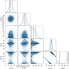 |
Fig. C.1 MCMC results using the CARMENES RVs obtained for GJ 3779. Each panel contains approximately 40 000 Keplerian samples. The upper panels of the corner plot show the probability density distributions of each orbital parameter. The vertical dashed lines indicate the mean and 1σ uncertainties of the fitted parameters. The rest of the panels show the dependencies between all the orbital elements in the parameter space. Black contours are drawn to improve the visualisation of the two-dimensional histograms. The distributions agree within the errors with the best-fit values from Table 2. |
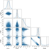 |
Fig. C.2 MCMC results using CARMENES and HARPS datasets obtained for GJ 1265. Each panel contains approximately 40 000 Keplerian samples. The quantities represented and the format of the plot are the same as in Fig. C.1. The distributions agree within the errors with the best-fit values from Table 2. |
References
- Affer, L., Micela, G., Damasso, M., et al. 2016, A&A, 593, A117 [NASA ADS] [CrossRef] [EDP Sciences] [Google Scholar]
- Anglada-Escudé, G., & Tuomi, M. 2012, A&A, 548, A58 [NASA ADS] [CrossRef] [EDP Sciences] [Google Scholar]
- Anglada-Escudé, G., Amado, P. J., Barnes, J., et al. 2016, Nature, 536, 437 [NASA ADS] [CrossRef] [PubMed] [Google Scholar]
- Astudillo-Defru, N., Forveille, T., Bonfils, X., et al. 2017a, A&A, 602, A88 [NASA ADS] [CrossRef] [EDP Sciences] [Google Scholar]
- Astudillo-Defru, N., Díaz, R. F., Bonfils, X., et al. 2017b, A&A, 605, L11 [Google Scholar]
- Baluev, R. V. 2009, MNRAS, 393, 969 [NASA ADS] [CrossRef] [Google Scholar]
- Barnes, J. R., Jeffers, S. V., & Jones, H. R. A. 2011, MNRAS, 412, 1599 [NASA ADS] [CrossRef] [Google Scholar]
- Bayo, A., Rodrigo, C., Barrado Y., Navascués, D., et al. 2008, A&A, 492, 277 [NASA ADS] [CrossRef] [EDP Sciences] [Google Scholar]
- Benedict, G. F., Henry, T. J., Franz, O. G., et al. 2016, AJ, 152, 141 [NASA ADS] [CrossRef] [Google Scholar]
- Berta, Z. K., Irwin, J., Charbonneau, D., Burke, C. J., & Falco, E. E. 2012, AJ, 144, 145 [NASA ADS] [CrossRef] [Google Scholar]
- Berta-Thompson, Z. K., Irwin, J., Charbonneau, D., et al. 2015, Nature, 527, 204 [NASA ADS] [CrossRef] [PubMed] [Google Scholar]
- Bonfils, X., Forveille, T., Delfosse, X., et al. 2005, A&A, 443, L15 [NASA ADS] [CrossRef] [EDP Sciences] [Google Scholar]
- Bonfils, X., Gillon, M., Forveille, T., et al. 2011, A&A, 528, A111 [NASA ADS] [CrossRef] [EDP Sciences] [Google Scholar]
- Bonfils, X., Delfosse, X., Udry, S., et al. 2013, A&A, 549, A109 [NASA ADS] [CrossRef] [EDP Sciences] [Google Scholar]
- Bonfils, X., Astudillo-Defru, N., Díaz, R., et al. 2018, A&A, 613, A25 [NASA ADS] [CrossRef] [EDP Sciences] [Google Scholar]
- Caballero, J. A., Cortés-Contreras, M., Alonso-Floriano, F. J., et al. 2016, 19th Cambridge Workshop on Cool Stars, Stellar Systems, and the Sun (CS19), 148 [Google Scholar]
- Charbonneau, D., Irwin, J., Nutzman, P., & Falco, E. E. 2008, AAS Meeting Abstracts, 212, 44.02 [Google Scholar]
- Charbonneau, D., Berta, Z. K., Irwin, J., et al. 2009, Nature, 462, 891 [NASA ADS] [CrossRef] [PubMed] [Google Scholar]
- Cortés-Contreras, M. 2016, Ph.D. Thesis, Universidad Complutense de Madrid, Spain [Google Scholar]
- Delfosse, X., Forveille, T., Ségransan, D., et al. 2000, A&A, 364, 217 [NASA ADS] [Google Scholar]
- Dressing, C. D., & Charbonneau, D. 2015, ApJ, 807, 45 [NASA ADS] [CrossRef] [Google Scholar]
- Foreman-Mackey, D., Hogg, D. W., Lang, D., & Goodman, J. 2013, PASP, 125, 306 [CrossRef] [Google Scholar]
- Forveille, T., Bonfils, X., Delfosse, X., et al. 2009, A&A, 493, 645 [NASA ADS] [CrossRef] [EDP Sciences] [Google Scholar]
- Fulton, B. J., & Petigura, E. A. 2018, AJ, 156, 264 [NASA ADS] [CrossRef] [Google Scholar]
- Fulton, B. J., Petigura, E. A., Howard, A. W., et al. 2017, AJ, 154, 109 [NASA ADS] [CrossRef] [Google Scholar]
- Gaia Collaboration (Brown, A. G. A., et al.) 2018, A&A, 616, A1 [NASA ADS] [CrossRef] [EDP Sciences] [Google Scholar]
- Gaidos, E., Mann, A. W., Kraus, A. L., & Ireland, M. 2016, MNRAS, 457, 2877 [NASA ADS] [CrossRef] [Google Scholar]
- Gillon, M., Triaud, A. H. M. J., Demory, B.-O., et al. 2017, Nature, 542, 456 [NASA ADS] [CrossRef] [PubMed] [Google Scholar]
- Grimm, S. L., Demory, B.-O., Gillon, M., et al. 2018, A&A, 613, A68 [NASA ADS] [CrossRef] [EDP Sciences] [Google Scholar]
- Hawley, S. L., Gizis, J. E., & Reid, I. N. 1996, AJ, 112, 2799 [NASA ADS] [CrossRef] [Google Scholar]
- Henry, T. J., Jao, W.-C., Winters, J. G., et al. 2016, AAS Meeting Abstracts, 227, 142.01 [Google Scholar]
- Hirano, T., Dai, F., Gandolfi, D., et al. 2018, AJ, 155, 127 [NASA ADS] [CrossRef] [Google Scholar]
- Husser, T.-O., Wende-von Berg, S., Dreizler, S., et al. 2013, A&A, 553, A6 [NASA ADS] [CrossRef] [EDP Sciences] [Google Scholar]
- Jeffers, S. V., Schöfer, P., Lamert, A., et al. 2018, A&A, 614, A76 [NASA ADS] [CrossRef] [EDP Sciences] [Google Scholar]
- Kaminski, A., Trifonov, T., Caballero, J. A., et al. 2018, A&A, 618, A115 [NASA ADS] [CrossRef] [EDP Sciences] [Google Scholar]
- Kane, S. R., Mahadevan, S., von Braun, K., Laughlin, G., & Ciardi, D. R. 2009, PASP, 121, 1386 [NASA ADS] [CrossRef] [Google Scholar]
- Kopparapu, R. K., Ramirez, R., Kasting, J. F., et al. 2013, ApJ, 765, 131 [NASA ADS] [CrossRef] [Google Scholar]
- Kopparapu, R. K., Ramirez, R. M., SchottelKotte, J., et al. 2014, ApJ, 787, L29 [NASA ADS] [CrossRef] [Google Scholar]
- Kovács, G., Zucker, S., & Mazeh, T. 2002, A&A, 391, 369 [NASA ADS] [CrossRef] [EDP Sciences] [Google Scholar]
- Marcy, G. W., Butler, R. P., Vogt, S. S., Fischer, D., & Lissauer, J. J. 1998, ApJ, 505, L147 [NASA ADS] [CrossRef] [Google Scholar]
- Mayor, M., Pepe, F., Queloz, D., et al. 2003, The Messenger, 114, 20 [NASA ADS] [Google Scholar]
- Neves, V., Bonfils, X., Santos, N. C., et al. 2014, A&A, 568, A121 [NASA ADS] [CrossRef] [EDP Sciences] [Google Scholar]
- Newton, E. R., Charbonneau, D., Irwin, J., et al. 2014, AJ, 147, 20 [NASA ADS] [CrossRef] [Google Scholar]
- Passegger, V. M., Wende-von Berg, S., & Reiners, A. 2016, A&A, 587, A19 [NASA ADS] [CrossRef] [EDP Sciences] [Google Scholar]
- Passegger, V. M., Reiners, A., Jeffers, S. V., et al. 2018, A&A, 615, A6 [NASA ADS] [CrossRef] [EDP Sciences] [Google Scholar]
- Perger, M., Ribas, I., Damasso, M., et al. 2017, A&A, 608, A63 [NASA ADS] [CrossRef] [EDP Sciences] [Google Scholar]
- Press, W. H., Teukolsky, S. A., Vetterling, W. T., & Flannery, B. P. 1992, Numerical Recipes in FORTRAN. The Art of Scientific Computing (Cambridge: University Press) [Google Scholar]
- Queloz, D., Henry, G. W., Sivan, J. P., et al. 2001, A&A, 379, 279 [NASA ADS] [CrossRef] [EDP Sciences] [Google Scholar]
- Quirrenbach, A., Amado, P. J., Caballero, J. A., et al. 2014, in Ground-based and Airborne Instrumentation for Astronomy V, Proc. SPIE, 9147, 91471F [Google Scholar]
- Reiners, A., Schüssler, M., & Passegger, V. M. 2014, ApJ, 794, 144 [NASA ADS] [CrossRef] [Google Scholar]
- Reiners, A., Ribas, I., Zechmeister, M., et al. 2018a, A&A, 609, L5 [Google Scholar]
- Reiners, A., Zechmeister, M., Caballero, J. A., et al. 2018b, A&A, 612, A49 [NASA ADS] [CrossRef] [EDP Sciences] [Google Scholar]
- Ricker, G. R., Winn, J. N., Vanderspek, R., et al. 2014, in Space Telescopes and Instrumentation 2014: Optical, Infrared, and Millimeter Wave, Proc. SPIE, 9143, 914320 [Google Scholar]
- Rivera, E. J., Lissauer, J. J., Butler, R. P., et al. 2005, ApJ, 634, 625 [NASA ADS] [CrossRef] [Google Scholar]
- Robertson, P., Mahadevan, S., Endl, M., & Roy, A. 2014, Science, 345, 440 [NASA ADS] [CrossRef] [Google Scholar]
- Rosen, S. R., Webb, N. A., Watson, M. G., et al. 2016, A&A, 590, A1 [NASA ADS] [CrossRef] [EDP Sciences] [Google Scholar]
- Sarkis, P., Henning, T., Kürster, M., et al. 2018, AJ, 155, 257 [NASA ADS] [CrossRef] [Google Scholar]
- Skrutskie, M. F., Cutri, R. M., Stiening, R., et al. 2006, AJ, 131, 1163 [NASA ADS] [CrossRef] [Google Scholar]
- Suárez Mascareño, A., González Hernández, J. I., Rebolo, R., et al. 2017, A&A, 597, A108 [NASA ADS] [CrossRef] [EDP Sciences] [Google Scholar]
- Tal-Or, L., Zechmeister, M., Reiners, A., et al. 2018, A&A, 614, A122 [NASA ADS] [CrossRef] [EDP Sciences] [Google Scholar]
- Trifonov, T., Kürster, M., Zechmeister, M., et al. 2018, A&A, 609, A117 [NASA ADS] [CrossRef] [EDP Sciences] [Google Scholar]
- Udry, S., Bonfils, X., Delfosse, X., et al. 2007, A&A, 469, L43 [NASA ADS] [CrossRef] [EDP Sciences] [Google Scholar]
- Vanderburg, A., & Johnson, J. A. 2014, PASP, 126, 948 [NASA ADS] [CrossRef] [Google Scholar]
- West, A. A., Weisenburger, K. L., Irwin, J., et al. 2015, ApJ, 812, 3 [NASA ADS] [CrossRef] [Google Scholar]
- Wright, J. T., & Eastman, J. D. 2014, PASP, 126, 838 [NASA ADS] [CrossRef] [EDP Sciences] [Google Scholar]
- Wright, D. J., Wittenmyer, R. A., Tinney, C. G., Bentley, J. S., & Zhao, J. 2016, ApJ, 817, L20 [NASA ADS] [CrossRef] [Google Scholar]
- Zechmeister, M., & Kürster, M. 2009, A&A, 496, 577 [NASA ADS] [CrossRef] [EDP Sciences] [Google Scholar]
- Zechmeister, M., Kürster, M., & Endl, M. 2009, A&A, 505, 859 [NASA ADS] [CrossRef] [EDP Sciences] [Google Scholar]
- Zechmeister, M., Reiners, A., Amado, P. J., et al. 2018, A&A, 609, A12 [CrossRef] [Google Scholar]
For the sake of clarity, we only show the full GLS periodogram up to 1 d-1 in Fig. A.1.
All Tables
All Figures
|
Fig. 1 K2 light curve of GJ 1265. The photometric variability of the star is longer than the 69 d baseline of the observations. |
| In the text | |
|
Fig. 2 GLS periodograms for GJ 3779 CARMENES RVs (panel a) and its residuals (panel b) after removing the prominent peak at f = 0.3307 d-1 (P = 3.023 d), marked in red. Panel c: periodogram of a photometric campaign of MEarth data from 2010. The highest peak at frot = 0.0105 d-1 (P = 95.2 d) associatedwith the star’s rotation is marked with a solid blue line and its first harmonic (2frot) with a dashed blue line. Panels d–f: periodograms of the chromatic index, differential line width, and Hα index, while panels g–i show periodograms for the cross-correlation function FWHM, contrast, and bisector velocity span. Horizontal lines show the theoretical FAP levels of 10%(short-dashed line), 1% (long-dashed line), and 0.1% (dot-dashed line) for each panel. |
| In the text | |
|
Fig. 3 CARMENES RVs and residuals phase-folded to the best Keplerian fitconsistent with a 3.023 d period planet around GJ 3779. |
| In the text | |
|
Fig. 4 Phase-folded light curve to the 3.023 d planet period of the MEarth photometric data for GJ 3779. The grey shaded area marks the expected transit duration. The central time of the expected transit is also marked with a vertical bar. |
| In the text | |
|
Fig. 5 GLS periodograms for GJ 1265 CARMENES (panel a), HARPS (panel b), and combined CARMENES+HARPS (panel c) data. Panel d: residuals after removing the prominent peak at f = 0.2739 d-1 (P = 3.651 d) marked in red. The blue shaded area depicts the excluded planetary region due to stellar variability as discussed in Sect. 3. Panels e–j and horizontal lines are the same as in Fig. 2. |
| In the text | |
|
Fig. 6 CARMENES (orange) and HARPS (green) radial velocities and residuals phase-folded to the best Keplerian fit consistent with a planet around GJ 1265 with a period of 3.651 d. |
| In the text | |
|
Fig. 7 Phase-folded light curve to the 3.651 d planet period of the K2 photometric data for GJ 1265. The grey shaded area marks the expected transit duration. The central time of the expected transit is also marked with a vertical bar. |
| In the text | |
|
Fig. 8 Mass-period diagram of all super-Earth planets, with masses determined from RVs or TTVs, orbiting mid- and late-type M dwarfs (left panel) and for all M dwarfs (right panel) taken from the NASA Exoplanet Archive from May 2018 (https://exoplanetarchive.ipac.caltech.edu). Single- and multi-planet systems are drawn with circles and triangles, respectively.The colorbar indicates the effective temperature of the host star. |
| In the text | |
|
Fig. A.1 Extended GLS periodograms for GJ 3779 (left panels) and GJ 1265 (right panels) covering the full frequency range. The magnitudes and the format represented are the same as in Figs. 2 and 5. |
| In the text | |
|
Fig. B.1 CARMENES VIS radial velocities against the chromatic index (CRX) for GJ 3779 (left panel) and GJ 1265 (right panel). The slopes of each linear fit are consistent with zero within the errors; activity-induced correlation is usually associated with a negative slope (Tal-Or et al. 2018). |
| In the text | |
|
Fig. C.1 MCMC results using the CARMENES RVs obtained for GJ 3779. Each panel contains approximately 40 000 Keplerian samples. The upper panels of the corner plot show the probability density distributions of each orbital parameter. The vertical dashed lines indicate the mean and 1σ uncertainties of the fitted parameters. The rest of the panels show the dependencies between all the orbital elements in the parameter space. Black contours are drawn to improve the visualisation of the two-dimensional histograms. The distributions agree within the errors with the best-fit values from Table 2. |
| In the text | |
|
Fig. C.2 MCMC results using CARMENES and HARPS datasets obtained for GJ 1265. Each panel contains approximately 40 000 Keplerian samples. The quantities represented and the format of the plot are the same as in Fig. C.1. The distributions agree within the errors with the best-fit values from Table 2. |
| In the text | |
Current usage metrics show cumulative count of Article Views (full-text article views including HTML views, PDF and ePub downloads, according to the available data) and Abstracts Views on Vision4Press platform.
Data correspond to usage on the plateform after 2015. The current usage metrics is available 48-96 hours after online publication and is updated daily on week days.
Initial download of the metrics may take a while.