| Issue |
A&A
Volume 620, December 2018
|
|
|---|---|---|
| Article Number | A155 | |
| Number of page(s) | 6 | |
| Section | Galactic structure, stellar clusters and populations | |
| DOI | https://doi.org/10.1051/0004-6361/201833367 | |
| Published online | 11 December 2018 | |
With and without spectroscopy: Gaia DR2 proper motions of seven ultra-faint dwarf galaxies⋆
Kapteyn Astronomical Institute, University of Groningen, AD Groningen 9747, The Netherlands
e-mail: This email address is being protected from spambots. You need JavaScript enabled to view it.
Received:
4
May
2018
Accepted:
15
October
2018
Abstract
Aims. We present mean absolute proper motion measurements for seven ultra-faint dwarf galaxies orbiting the Milky Way, namely Boötes III, Carina II, Grus II, Reticulum II, Sagittarius II, Segue 2, and Tucana IV. For four of these dwarfs our proper motion estimate is the first ever provided.
Methods. The adopted astrometric data come from the second data release of the Gaia mission. We determine the mean proper motion for each galaxy starting from an initial guess of likely members, based either on radial velocity measurements or using stars on the horizontal branch identified in the Gaia (GBP – GRP, G) colour-magnitude diagram in the field of view towards the UFD. We then refine their membership iteratively using both astrometry and photometry. We take into account the full covariance matrix among the astrometric parameters when deriving the mean proper motions for these systems.
Results. Our procedure provides mean proper motions with typical uncertainties of ∼0.1 mas yr−1, even for galaxies without prior spectroscopic information. In the case of Segue 2 we find that using radial velocity members only leads to biased results, presumably because of the small number of stars with measured radial velocities.
Conclusions. Our procedure allows the number of member stars per galaxy to be maximized regardless of the existence of prior spectroscopic information, and can therefore be applied to any faint or distant stellar system within reach of Gaia.
Key words: Galaxy: kinematics and dynamics / galaxies: dwarf / Local Group / astrometry / proper motions
Full Table 2 is only available at the CDS via anonymous ftp to cdsarc.u-strasbg.fr (130.79.128.5) or via http://cdsarc.u-strasbg.fr/viz-bin/qcat?J/A+A/620/A155
© ESO 2018
1. Introduction
The orbits of the satellite galaxies of the Milky Way constitute a powerful tool to answer several important questions of modern astrophysics. They provide valuable constraints on the mass and shape of the Milky Way halo (Little & Tremaine 1987; Wilkinson & Evans 1999), as well as on the evolution of the satellites themselves and their resilience to tidal forces (Peñarrubia et al. 2008; Łokas et al. 2012). Orbits also allow us to investigate whether their dynamical evolution and star formation histories are connected (Grebel 2001; Tolstoy et al. 2004; Battaglia et al. 2008). Furthermore, they reveal how our Galaxy has assembled its population of dwarf galaxy satellites (Kroupa et al. 2005; Li & Helmi 2008), and how this process relates to the large-scale environment in which the Galaxy is embedded (Libeskind et al. 2005; Buck et al. 2016).
To determine the orbits of Milky Way satellites, their position on the sky, distance, line of sight velocity, and proper motions are required. Historically, the last two observables of this six-dimensional phase space have been the most difficult to measure. Only recently and mostly thanks to the exquisite astrometric capabilities of the Hubble Space Telescope (HST), have absolute proper motions been provided for many of the brightest dwarf galaxies orbiting our Galaxy (e.g. Piatek et al. 2003; Massari et al. 2013; Kallivayalil et al. 2013; Sohn et al. 2013, 2017).
The advent of the Gaia mission (Gaia Collaboration 2016a,b) has resulted in a quantum leap in our ability to measure proper motions for distant stellar systems. Already with its first data release, thanks to the combination with pre-existing datasets such as Tycho, HST or the Sloan Digital Sky Survey, Gaia has enabled measurements of the proper motions of Galactic globular clusters (Massari et al. 2017; Watkins & van der Marel 2017), stellar streams (Helmi et al. 2017; Deason et al. 2018), and stars in dwarf spheroidal galaxies (Massari et al. 2018). Yet, it is with the second data release (DR2; Gaia Collaboration 2018a), that Gaia becomes transformational. The Gaia DR2 catalogue contains absolute proper motions for more than one billion stars, and this has permitted for the first time direct measurement of proper motions over the full sky and without the need for external objects for absolute calibration. This has resulted in spectacularly precise proper motion estimates for 75 Galactic globular clusters, the Large and the Small Magellanic Clouds, the nine classical dwarf spheroidal galaxies, and one ultra-faint dwarf galaxy (UFD; Gaia Collaboration 2018b).
Results for the seven UFDs analysed in this paper.
Ultra-faint galaxies are very difficult objects to detect because of their low luminosity, but the number of known UFDs is continuously increasing thanks to wide-field deep surveys (e.g. Drlica-Wagner et al. 2015; Laevens et al. 2015; Torrealba et al. 2018). Ultra-faint galaxies might well constitute one of the best solutions to the missing-satellites problem (Moore et al. 1999; Klypin et al. 1999). Despite their cosmological importance, very little is known about their origin, and knowledge of their orbits around the Milky Way is a powerful way to find clues. Until very recently, only two UFDs had an absolute proper motion measurement (Fritz et al. 2018a; Gaia Collaboration 2018b). Around the time of submission of this paper, several new investigations reported absolute proper motions for UFDs using stars defined as members based on radial velocity measurements (Simon 2018; Fritz et al. 2018b; Kallivayalil et al. 2018; Carlin & Sand 2018). However, relying on spectroscopic information only is not entirely advisable. It limits the number of UFDs whose proper motions can be determined, as not all UFDs have been followed up spectroscopically (see also Pace & Li 2018). Furthermore, as we show here, it might lead to biased results because of small sample sizes and therefore poor statistical significance.
In this paper we present the absolute proper motion for seven UFDs, namely Boötes III, Carina II, Grus II, Reticulum II, Sagittarius II, Segue 2, and Tucana IV. All of these are located within 70 kpc of the earth and have an integrated absolute V-band magnitude brighter than MV = −2.5. Four out of these seven UFDs do not have publicly available spectroscopic information. We develop a method to reliably select likely members even in such cases, and show that this method also fares better on UFDs with spectroscopic information, because it allows us to infer a more complete sample of members that is not limited to stars with measured radial velocities.
IDs and sky positions for stellar members of each UFD.
2. Stellar membership and mean proper motion determination
In a recent paper, Simon (2018) determined the mean proper motion for 17 UFDs by using all the stars defined as members according to their radial velocities. However, this kind of information is not available for the entire sample of Milky Way dwarf satellites. Moreover, spectroscopic samples are incomplete by nature being limited to small numbers of stars, and this can potentially lead to biased mean proper motion estimates (see below). For these reasons, in this paper we develop a procedure that is less prone to these issues, and which we use to determine stellar membership and mean proper motions of each of the analysed UFDs.
Our procedure is iterative and consists of the following steps that are applied to each one of the UFDs:
We identify initial likely members from either spectroscopic (radial velocity member candidates) or photometric (horizontal branch (HB) candidates) information.
From the initial set of likely members, we estimate mean proper motions (〈μα cos δ〉, 〈μδ〉) and parallax 〈ϖ〉, together with the corresponding standard deviations (σμα, σμδ, σϖ).
We apply a 2.5σ selection around these mean astrometric parameters.
We perform a further selection on i) the colour-magnitude diagram (see e.g. the blue box in Fig. 3), ii) projected distance from the centre of the UFD, and iii) we exclude stars with 0 < σϖ/ϖ < 0.2 to remove obvious very nearby foreground contaminants.
The stars that survive these selection criteria are defined as new likely members, and their mean astrometric parameters and associated uncertainty (defined as the root mean square around the mean) are determined.
We repeat steps 3, 4, and 5 until convergence is reached. Convergence is defined as the point where the change between the mean astrometric parameters in two subsequent iterations is smaller than 0.5 times the previously determined root mean square (rms) error.
The convergence of the whole procedure, especially for the cases of poorly populated UFDs or when the contamination of the surrounding field is strong, depends on the adopted projected distance cut. The choice of the projected distance cut results from a balance between avoiding excessive contamination and including the largest possible number of members. We find that the best solution is different for each single UFD, and we applied cuts ranging from ∼3.5′ for the most crowded case (Sagittarius II) to ∼20′ for the most diffuse UFDs (see the red circles in Figs. 2 and 5). The mean proper motions obtained in the last step are adopted as the final solution.
We underline that the mean proper motions of the UFDs have been computed by taking into account the correlations among the astrometric parameter uncertainties for each of the stars following the method developed by van Leeuwen (2009) and described in detail in Appendix A.1 of Gaia Collaboration (2017)1. We find that not properly including these correlations results in systematic errors that can be as large as ∼0.05 mas yr−1.
In the following section we present the results obtained by following this procedure when applied to our sample of seven UFDs. We first focus on the dwarfs that have spectroscopic follow-up such that the initial guess is based on radial velocity determinations, and then on those UFDs for which we use HB stars. In Table 1 we list the resulting proper motions 〈μα cos δ〉, 〈μδ〉, the associated uncertainties (defined as the rms error around the mean), covariance, and the number of final members used for all of the seven UFDs. We stress that, though not reported in this analysis, systematic errors on the mean proper motion estimates as large as ∼0.035 mas yr−1 are expected to act on the small scales sampled in this work (see e.g. Sect. 4.1 in Gaia Collaboration 2018b, Sect. 4.2 in Arenou et al. 2018 and Sect. 5.4 in Lindegren et al. 2018). The list of IDs and positions of our final members for each UFD is made publicly available through the CDS. An example showing the first four members of each galaxy is given in Table 2.
3. Results: UFDs with spectroscopic information
In our sample of dwarfs, Carina II, Reticulum II, and Segue 2 have radial velocity measurements available in the literature (see Li et al. 2018; Simon et al. 2015; Koposov et al. 2015; Kirby et al. 2013). Therefore, for these three dwarfs we cross-matched their membership lists with the Gaia DR2 catalogue and used the stars in common for the first step of our procedure. The location of these stars in the vector point diagrams (VPDs) is shown as cyan filled circles in Fig. 1.
We then applied our procedure which converges quickly, that is, after two to three iterations. The final sample of member stars is marked by the red filled circles in the same figure. As expected this figure shows that the number of members we find is larger than that coming only from the spectroscopic data. Moreover, a few of the radial velocity candidate members turned out to be false members, and these are shown with the cyan empty circles in Fig. 2. These stars are excluded from the final computation of the mean proper motions, which are therefore more accurate also because of the larger number of true members.
The step-wise procedure we follow therefore constitutes a big improvement, and the case of Segue 2 demonstrates this. For this system, the distribution of spectroscopic members in the VPD is significantly shifted towards larger μα cos δ and larger μδ in comparison to the rest of the stars that we identify as members. This results in a small discrepancy between Simon (2018) and our own measurement: our derived mean proper motion is (〈μα cos δ〉, 〈μδ〉) = (1.27 ± 0.11, −0.10 ± 0.15)mas yr−1, which is ∼1.5σ away from the value quoted in Simon (2018).
On the other hand, the VPD distribution of spectroscopic members for Carina II and Reticulum II seems to represent well the overall population as determined by our procedure. In fact, our results match within 1σ those in Simon (2018), Fritz et al. (2018b) and Kallivayalil et al. (2018), being (〈μα cos δ〉, 〈μδ〉) = (1.81 ± 0.08, 0.14 ± 0.08)mas yr−1 for Carina II and (〈μα cos δ〉, 〈μδ〉) = (2.34 ± 0.12, −1.31 ± 0.13)mas yr−1 for Reticulum II. The small remaining differences might be explained by differences in the (often larger) sample of members produced by our procedure, and by the fact that we took into account the correlations among the astrometric parameters (see Arenou et al. 2018 and Fig. A.11 in Gaia Collaboration 2018b), as well as by the use of a standard mean instead of a weighted mean.
The distribution on the sky of our selected members is a consistency check validating the robustness of our selection procedure, and is also extremely interesting from a scientific point of view. We should reasonably expect that, if our selection works properly, the selected members of each galaxy define an overdensity with respect to field stars in their distribution in right ascention (α) and declination (δ). This is indeed nicely shown in Fig. 2.
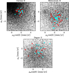 |
Fig. 1. VPDs for the stars in the direction of the three UFDs with published radial velocity catalogues. Cyan filled circles mark the spectroscopic members. Red filled circles highlight all the stars defined as members at the end of the procedure described in Sect. 2. Black dots show all the stars in a field of view of 3° radius from the centres of the UFDs. |
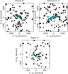 |
Fig. 2. Location on the sky of stars surviving the last iterative step of the membership procedure. For the sake of representation, the distance cut has not been applied but is marked with a red circle. Cyan empty circles mark initial radial velocity candidate members. |
For all three UFDs, the members (black filled circles within the projected distance cut shown as a red circle) define relatively elongated or asymmetric structures, suggestive of tidal effects acting on these UFDs and affecting their shape. Such features were already recognised in the Magellanic Satellite Survey photometry of Carina II (Torrealba et al. 2018), the Dark Energy Survey photometry of Reticulum II (Bechtol et al. 2015), and the Sloan Extension for Galactic Understanding and Exploration of Segue 2 (Belokurov et al. 2009). While in those cases the field decontamination was based on statistical methods, here it relies on kinematically observed properties and is therefore more robust. Nonetheless the similarities between the shapes of the sky distributions obtained in the different ways are remarkable.
4. Results: UFDs without spectroscopic information
The UFDs Boötes III, Grus II, Sagittarius II and Tucana IV do not have publicly available spectroscopic information. As mentioned in Sect. 2 we therefore use HB candidates located within 15′ of the centre of each UFD (from McConnachie 2012) to obtain an initial guess on the mean astrometric parameters. Horizontal branch stars have been chosen because they are easy to detect in the CMD, being bluer than the typical sequences described by the majority of stars located in the respective fields of view. This is clearly demonstrated in Fig. 3, where the CMD regions adopted to select HB stars are marked with a cyan box.
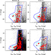 |
Fig. 3. CMDs for the field of view around the four UFDs with no available spectroscopic information. The cyan box highlights the region where HB candidates were initially selected. Red filled circles mark the final list of members, again without applying the CMD selection but representing it with the blue box. |
To demonstrate the effectiveness of the selection procedure described in Sect. 2, Fig. 3 shows a snapshot of the last iteration step from the point of view of the CMD. The red filled circles are stars that survived the 2.5σ-clipping astrometric selection and items 4ii) and 4iii) of the procedure. However, only those located inside the blue delimited box are used for the final mean proper motion estimate. In general, the selected members are located on the typical evolutionary sequences characteristic of the stellar populations seen in dwarf galaxies. These sequences are relatively well-defined despite the meagre numbers (40–50 stars). The fact that the poorly populated red giant branches are also quite faint (the brightest HB is at G ∼ 19) contributes to spreading them out in GBP – GRP colour. The colour uncertainty at these magnitudes is ∼0.1, whereas the measured spread amounts to ∼0.15. Therefore we cannot exclude the presence of multiple, possibly chemically heterogeneous sub-populations (in fact UFDs typically show spread in their metallicity distribution; see Tolstoy et al. 2009).
The distribution in the VPD of the final members of the four UFD galaxies is shown in Fig. 4 with red filled circles. As for the dwarfs analysed in Sect. 3, they describe a reasonably well-concentrated clump of stars, clearly separated from the bulk of the field population (black dots). It is interesting to note that in the case of Boötes III, a third concentration of stars clearly stands out at (〈μα cos δ〉, 〈μδ〉) ∼ (−5, −1) mas yr−1; it is made up of stars belonging to the Galactic globular cluster NGC 5466, located very close to the galaxy also on the sky. Their quite different distances from the Sun (with the UFD ∼30 kpc farther away, Ferraro et al. 1999) and kinematics, with Boötes III having (〈μα cos δ〉, 〈μδ〉) = (−1.21 ± 0.13, −0.92 ± 0.17)mas yr−1, corresponding to a difference in velocity of about 100 km s−1, implies that the two systems are not associated to each other.
The spreads in the distributions of members in the VPDs of the four UFDs are consistent with the typical proper motion uncertainties of their stars. This is true even for the case of Sagittarius II, whose distribution seems significantly more extended and asymmetric than for the other systems. This is because for its stars, the errors on μα cos δ are a factor of ∼1.5 larger than those on μδ. The cyan filled circles in Fig. 4 mark the initial HB candidates, most of them being located well within the region of the final members.
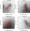 |
Fig. 4. VPDs for the stars around the four UFDs. Red filled circles mark stars belonging to the final list of members. |
Finally, Fig. 5 shows the distribution of the selected members on the sky. As in Sect. 3, only stars represented as black dots and within the red circle have been considered for the final mean proper motion estimate. All four galaxies show a peak in the concentration of their members within the projected distance cut given by the radius of the red circle. Interestingly however, for some of these (namely Boötes III and Tucana IV), the peak of the density distribution seems somewhat offset with respect to the nominal centre (given by the centre of the red circle, and taken from Grillmair 2009 and Drlica-Wagner et al. 2015, respectively). Moreover, all the systems, with the possible exception of Sagittarius II (which has been proposed to be a globular cluster rather than a UFD; see Mutlu-Pakdil et al. 2018), appear asymmetric and possibly depict an elongated shape. It is beyond the aim of this paper to make a quantitative analysis on these aspects, yet our findings already highlight how powerful Gaia can be to better assess the density profiles and centres of systems like the UFDs, which suffer from large amounts of contamination by field stars.
The location of all the initially selected candidate HB stars are marked in Fig. 5 with cyan empty circles. A few of these HB stars were lost during the procedure, but this was to be expected given that the initial selection is astrometrically blind. The fact that the actual members all lie well within the adopted projected distance cut from the nominal centre is a further verification of the robustness of our procedure. Sagittarius II might show hints of the presence of a few HB members outside this distance cut. Increasing such a radius does not improve the final proper motion estimate, and given the high degree of contamination in that field we cannot conclude whether or not they are false members.
5. Summary
In this paper we have estimated the mean absolute proper motion for seven UFD satellites of the Milky Way, all located within 70 kpc from the earth and with an integrated V-band magnitude brighter than V = 15. This has ensured that a sufficiently large number of members are above Gaia magnitude limit of G ≃ 21. For four of these seven dwarfs, ours is the first proper motion estimate ever provided.
To determine likely member stars from which to compute the mean proper motion of each system we developed a new procedure which proved to be less prone to systematic uncertainties than using only radial velocity members when the sample size is very small. This procedure starts from an initial guess on the mean proper motion and parallax coming from an initial sample of tentative members, and then refines their membership and the mean astrometric parameters by coupling photometric (CMD selection) and astrometric information together. The initial sample of candidate members is made up of spectroscopic members, if radial velocity measurements are publicly available, or HB stars otherwise.
For all seven UFDs studied here, our procedure works well. We obtain well-defined evolutionary sequences in the CMDs and a clear concentration of stars in the VPDs. Interestingly, the distribution on the sky of the selected members often highlights elongated or asymmetric structures, suggestive of tidal perturbations or complex dynamical histories, and a couple of galaxies might be offset with respect to their previously determined density centres. Future investigations based on Gaia photometric and astrometric datasets, possibly in combination with dynamical models, will be used to assess these findings.
When comparing our results to those of Simon (2018) and Fritz et al. (2018b) for the sub-sample of UFDs with spectroscopic information, we find good agreement for Carina II and Reticulum-II, where small differences can be ascribed to the different sample of members used (ours not being limited to spectroscopic members only) and to the fact that we took into account the full covariance matrix in the determination of the mean proper motions. On the other hand, we found a ∼1.5σ difference with the results of Simon (2018) for Segue 2, a system that this author recognised as peculiar due to the wide spread of its stars in the VPD. In this case, the sub-sample of spectroscopic members turns out to be systematically shifted in the VPD. This demonstrates that when limited to small samples, systematic effects related to small number statistics can bias the results.
In the case of UFDs without public spectroscopic information, we find good agreement for Boötes III with the results of Carlin & Sand (2018), who used proprietary radial velocities to assess the stellar membership and found a mean proper motion which matches ours well within a 1σ uncertainty. This is possibly the best confirmation on the validity of our method. Finally, our estimates on Grus II and Tucana IV agree well with those of Pace & Li (2018), both in terms of mean proper motions and of the expected number of members.
We have shown that thanks to Gaia, measurements of the absolute proper motions of many of the known UFD satellites of the Milky Way are within reach. This means that several of the questions relating to the nature and evolution of these systems will likely soon be answered.
We note that we neglected the terms in the covariance matrix related to the UFDs instrinsic parallax and proper motion dispersion because our targets are tens of kiloparsecs away from us.
Acknowledgments
We thank the referee for their report and suggestions which helped us to improve the quality of the paper. DM and AH acknowledge financial support from a Vici grant from NWO. This work has made use of data from the European Space Agency (ESA) mission Gaia (http://www.cosmos.esa.int/gaia), processed by the Gaia Data Processing and Analysis Consortium (DPAC, http://www.cosmos.esa.int/web/gaia/dpac/consortium). Funding for the DPAC has been provided by national institutions, in particular the institutions participating in the Gaia Multilateral Agreement.
References
- Arenou, F., Luri, X., Babusiaux, C., et al. 2018, A&A, 616, A17 [Google Scholar]
- Battaglia, G., Helmi, A., Tolstoy, E., et al. 2008, ApJ, 681, L13 [NASA ADS] [CrossRef] [Google Scholar]
- Bechtol, K., Drlica-Wagner, A., Balbinot, E., et al. 2015, ApJ, 807, 50 [NASA ADS] [CrossRef] [Google Scholar]
- Belokurov, V., Walker, M. G., Evans, N. W., et al. 2009, MNRAS, 397, 1748 [NASA ADS] [CrossRef] [Google Scholar]
- Buck, T., Dutton, A. A., & Macciò, A. V. 2016, MNRAS, 460, 4348 [NASA ADS] [CrossRef] [Google Scholar]
- Carlin, J. L., & Sand, D. J. 2018, ApJ, 865, 7 [NASA ADS] [CrossRef] [Google Scholar]
- Deason, A. J., Belokurov, V., & Koposov, S. E. 2018, MNRAS, 473, 2428 [NASA ADS] [CrossRef] [Google Scholar]
- Drlica-Wagner, A., Bechtol, K., Rykoff, E. S., et al. 2015, ApJ, 813, 109 [NASA ADS] [CrossRef] [Google Scholar]
- Ferraro, F. R., Messineo, M., Fusi Pecci, F., et al. 1999, AJ, 118, 1738 [NASA ADS] [CrossRef] [Google Scholar]
- Fritz, T. K., Lokken, M., Kallivayalil, N., et al. 2018a, ApJ, 860, 164 [NASA ADS] [CrossRef] [Google Scholar]
- Fritz, T. K., Battaglia, G., Pawlowski, M. S., et al. 2018b, A&A, 619, A103 [NASA ADS] [CrossRef] [EDP Sciences] [Google Scholar]
- Gaia Collaboration (Prusti, T., et al.) 2016a, A&A, 595, A1 [NASA ADS] [CrossRef] [EDP Sciences] [Google Scholar]
- Gaia Collaboration (Brown, A. G. A., et al.) 2016b, A&A, 595, A2 [NASA ADS] [CrossRef] [EDP Sciences] [Google Scholar]
- Gaia Collaboration (van Leeuwen, F., et al.) 2017, A&A , 601, A19 [NASA ADS] [CrossRef] [EDP Sciences] [Google Scholar]
- Gaia Collaboration (Brown, A. G. A., et al.) 2018a, A&A, 616, A1 [NASA ADS] [CrossRef] [EDP Sciences] [Google Scholar]
- Gaia Collaboration (Helmi, A., et al.) 2018b, A&A, 616, A12 [NASA ADS] [CrossRef] [EDP Sciences] [Google Scholar]
- Grebel, E. K. 2001, Astrophys. Space Sci. Suppl., 277, 231 [NASA ADS] [CrossRef] [Google Scholar]
- Grillmair, C. J. 2009, ApJ, 693, 1118 [NASA ADS] [CrossRef] [Google Scholar]
- Helmi, A., Veljanoski, J., Breddels, M. A., Tian, H., & Sales, L. V. 2017, A&A, 598, A58 [NASA ADS] [CrossRef] [EDP Sciences] [Google Scholar]
- Kallivayalil, N., van der Marel, R. P., Besla, G., Anderson, J., & Alcock, C. 2013, ApJ, 764, 161 [NASA ADS] [CrossRef] [Google Scholar]
- Kallivayalil, N., Sales, L., Zivick, P., et al. 2018, ApJ, 867, 19 [NASA ADS] [CrossRef] [Google Scholar]
- Kirby, E. N., Boylan-Kolchin, M., Cohen, J. G., et al. 2013, ApJ, 770, 16 [NASA ADS] [CrossRef] [Google Scholar]
- Klypin, A., Kravtsov, A. V., Valenzuela, O., & Prada, F. 1999, ApJ, 522, 82 [Google Scholar]
- Koposov, S. E., Casey, A. R., Belokurov, V., et al. 2015, ApJ, 811, 62 [NASA ADS] [CrossRef] [Google Scholar]
- Kroupa, P., Theis, C., & Boily, C. M. 2005, A&A, 431, 517 [NASA ADS] [CrossRef] [EDP Sciences] [Google Scholar]
- Laevens, B. P. M., Martin, N. F., Bernard, E. J., et al. 2015, ApJ, 813, 44 [NASA ADS] [CrossRef] [Google Scholar]
- Li, Y.-S., & Helmi, A. 2008, MNRAS, 385, 1365 [NASA ADS] [CrossRef] [Google Scholar]
- Li, T. S., Simon, J. D., Pace, A. B., et al. 2018, ApJ, 857, 145 [NASA ADS] [CrossRef] [Google Scholar]
- Libeskind, N. I., Frenk, C. S., Cole, S., et al. 2005, MNRAS, 363, 146 [NASA ADS] [CrossRef] [Google Scholar]
- Lindegren, L., Hernández, J., Bombrun, A., et al. 2018, A&A, 616, A2 [NASA ADS] [CrossRef] [EDP Sciences] [Google Scholar]
- Little, B., & Tremaine, S. 1987, ApJ, 320, 493 [NASA ADS] [CrossRef] [Google Scholar]
- Łokas, E. L., Majewski, S. R., Kazantzidis, S., et al. 2012, ApJ, 751, 61 [NASA ADS] [CrossRef] [Google Scholar]
- Massari, D., Bellini, A., Ferraro, F. R., et al. 2013, ApJ, 779, 81 [NASA ADS] [CrossRef] [Google Scholar]
- Massari, D., Posti, L., Helmi, A., Fiorentino, G., & Tolstoy, E. 2017, A&A, 598, L9 [NASA ADS] [CrossRef] [EDP Sciences] [Google Scholar]
- Massari, D., Breddels, M. A., Helmi, A., et al. 2018, Nat. Astron., 2, 156 [NASA ADS] [CrossRef] [Google Scholar]
- McConnachie, A. W. 2012, AJ, 144, 4 [NASA ADS] [CrossRef] [Google Scholar]
- Moore, B., Ghigna, S., Governato, F., et al. 1999, ApJ, 524, L19 [Google Scholar]
- Mutlu-Pakdil, B., Sand, D. J., Carlin, J. L., et al. 2018, ApJ, 863, 25 [NASA ADS] [CrossRef] [Google Scholar]
- Pace, A. B., & Li, T. S. 2018, ApJ, submitted [arXiv:1806.02345] [Google Scholar]
- Pawlowski, M. S., & Kroupa, P. 2013, MNRAS, 435, 2116 [NASA ADS] [CrossRef] [Google Scholar]
- Peñarrubia, J., Navarro, J. F., & McConnachie, A. W. 2008, ApJ, 673, 226 [NASA ADS] [CrossRef] [Google Scholar]
- Piatek, S., Pryor, C., Olszewski, E. W., et al. 2003, AJ, 126, 2346 [Google Scholar]
- Sohn, S. T., Besla, G., van der Marel, R. P., et al. 2013, ApJ, 768, 139 [NASA ADS] [CrossRef] [Google Scholar]
- Sohn, S. T., Patel, E., Besla, G., et al. 2017, ApJ, 849, 93 [NASA ADS] [CrossRef] [Google Scholar]
- Simon, J. D. 2018, ApJ, 863, 89 [NASA ADS] [CrossRef] [Google Scholar]
- Simon, J. D., Drlica-Wagner, A., Li, T. S., et al. 2015, ApJ, 808, 95 [NASA ADS] [CrossRef] [Google Scholar]
- Torrealba, G., Belokurov, V., Koposov, S. E., et al. 2018, MNRAS, 475, 5085 [NASA ADS] [CrossRef] [Google Scholar]
- Tolstoy, E., Irwin, M. J., Helmi, A., et al. 2004, ApJ, 617, L119 [NASA ADS] [CrossRef] [Google Scholar]
- Tolstoy, E., Hill, V., & Tosi, M. 2009, ARA&A, 47, 371 [NASA ADS] [CrossRef] [Google Scholar]
- van Leeuwen, F. 2009, A&A, 497, 209 [NASA ADS] [CrossRef] [EDP Sciences] [Google Scholar]
- Watkins, L. L., & van der Marel, R. P. 2017, ApJ, 839, 89 [NASA ADS] [CrossRef] [Google Scholar]
- Wilkinson, M. I., & Evans, N. W. 1999, MNRAS, 310, 645 [NASA ADS] [CrossRef] [Google Scholar]
All Tables
All Figures
|
Fig. 1. VPDs for the stars in the direction of the three UFDs with published radial velocity catalogues. Cyan filled circles mark the spectroscopic members. Red filled circles highlight all the stars defined as members at the end of the procedure described in Sect. 2. Black dots show all the stars in a field of view of 3° radius from the centres of the UFDs. |
| In the text | |
|
Fig. 2. Location on the sky of stars surviving the last iterative step of the membership procedure. For the sake of representation, the distance cut has not been applied but is marked with a red circle. Cyan empty circles mark initial radial velocity candidate members. |
| In the text | |
|
Fig. 3. CMDs for the field of view around the four UFDs with no available spectroscopic information. The cyan box highlights the region where HB candidates were initially selected. Red filled circles mark the final list of members, again without applying the CMD selection but representing it with the blue box. |
| In the text | |
|
Fig. 4. VPDs for the stars around the four UFDs. Red filled circles mark stars belonging to the final list of members. |
| In the text | |
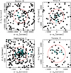 |
Fig. 5. As in Fig. 2 but for the four UFDs without spectroscopic information. |
| In the text | |
Current usage metrics show cumulative count of Article Views (full-text article views including HTML views, PDF and ePub downloads, according to the available data) and Abstracts Views on Vision4Press platform.
Data correspond to usage on the plateform after 2015. The current usage metrics is available 48-96 hours after online publication and is updated daily on week days.
Initial download of the metrics may take a while.