| Issue |
A&A
Volume 620, December 2018
|
|
|---|---|---|
| Article Number | A148 | |
| Number of page(s) | 21 | |
| Section | Stellar atmospheres | |
| DOI | https://doi.org/10.1051/0004-6361/201833298 | |
| Published online | 11 December 2018 | |
S stars and s-process in the Gaia era
I. Stellar parameters and chemical abundances in a sub-sample of S stars with new MARCS model atmospheres★
1
Institute of Astronomy and Astrophysics (IAA), Université libre de Bruxelles (ULB), CP 226,
Boulevard du Triomphe,
1050 Bruxelles, Belgium
e-mail: This email address is being protected from spambots. You need JavaScript enabled to view it.
2
Institute of Astronomy, KU Leuven, Celestijnenlaan 200D,
3001 Leuven, Belgium
3
Indian Institute of Astrophysics, Koramangala,
Bangalore
560034,
Karnataka, India
4
Laboratoire Univers et Particules de Montpellier, Université de Montpellier, CNRS
34095,
Montpellier Cedex 05, France
Received:
24
April
2018
Accepted:
10
October
2018
Abstract
Context. S stars are transition objects between M-type giants and carbon stars on the asymptotic giant branch (AGB). They are characterized by overabundances of s-process elements. Roughly half of them are enhanced in technetium (Tc), an s-process element with no stable isotope, while the other half lack technetium. This dichotomy arises from the fact that Tc-rich S stars are intrinsically producing s-process elements and have undergone third dredge-up (TDU) events, while Tc-poor S stars owe their s-process overabundances to a past pollution by a former AGB companion which is now an undetected white dwarf, and since the epoch of the mass transfer, technetium has totally decayed.
Aims. Our aim is to analyse the abundances of S stars and gain insights into their evolutionary status and on the nucleosynthesis of heavy s-process elements taking place in their interior. In particular, the location of extrinsic and intrinsic S stars in the HR diagram will be compared with the theoretical onset of the TDU on the thermally pulsing AGB.
Methods. A sample of 19 S-type stars was analysed by combining HERMES high-resolution spectra, accurate Gaia Data Release 2 (GDR2) parallaxes, stellar-evolution models, and newly designed MARCS model atmospheres for S-type stars. Various stellar parameters impact the atmospheric structure of S stars, not only effective temperature, gravity, metallicity and microturbulence but also C/O and [s/Fe]. We show that photometric data alone are not sufficient to disentangle these parameters. We present a new automatic spectral-fitting method that allows one to constrain the range of possible atmospheric parameters.
Results. Combining the derived parameters with GDR2 parallaxes allows a joint analysis of the location of the stars in the Hertzsprung–Russell diagram and of their surface abundances. For all 19 stars, Zr and Nb abundances are derived, complemented by abundances of other s-process elements for the three Tc-rich S stars. These abundances agree within the uncertainties with nucleosynthesis predictions for stars of corresponding mass, metallicity and evolutionary stage. The Tc dichotomy between extrinsic and intrinsic S stars is seen as well in the Nb abundances: intrinsic, Tc-rich S stars are Nb-poor, whereas extrinsic, Tc-poor S stars are Nb-rich. Most extrinsic S stars lie close to the tip of the red giant branch (RGB), and a few are located along the early AGB. All appear to be the cooler analogues of barium stars. Barium stars with masses smaller than 2.5 M⊙ turn into extrinsic S stars on the RGB, because only for those masses does the RGB tip extend to temperatures lower than ~4200 K, which allows the ZrO bands distinctive of S-type stars to develop. On the contrary, barium stars with masses in excess of ~2.5 M⊙ can only turn into extrinsic S stars on the E-AGB, but those are short-lived, and thus rare. The location of intrinsic S stars in the HR diagram is compatible with them being thermally-pulsing AGB stars. Although nucleosynthetic model predictions give a satisfactory distribution of s-process elements, fitting at the same time the carbon and heavy s-element enrichments still remains difficult. Finally, the Tc-rich star V915 Aql is challenging as it points at the occurrence of TDU episodes in stars with masses as low as M ~ 1 M⊙.
Key words: stars: abundances / stars: AGB and post-AGB / Hertzsprung–Russell and C–M diagrams / nuclear reactions, nucleosynthesis, abundances / stars: interiors
Based on observations made with the Mercator Telescope, operated on the Island of La Palma by the Flemish Community, at the Spanish Observatorio del Roque de los Muchachos of the Instituto de Astrofísica de Canarias.
© ESO 2018
1 Introduction
S stars are late-type giants characterized by the presence of TiO and ZrO molecular bands in their optical spectrum (Merrill 1922). The carbon to oxygen ratio (C/O) of S stars lies in the range from 0.5 to just below unity. This indicates that they are transition objects between M-type giants (C/O ~ 0.4) and carbon stars (C/O > 1) on the asymptotic giant branch (AGB; Iben & Renzini 1983). The spectra of S stars also show signatures of an overabundance of s-process elements (Smith & Lambert 1990). The s-process is a slow neutron-capture process which is responsible for the production of approximately half of all the elements heavier than Fe (Käppeler et al. 2011). S-process elements are transported to the stellar surface of a thermally pulsing AGB (TP-AGB) star by a mixing process called third dredge-up (TDU). A TP-AGB star undergoes several thermal pulses which are recurrent thermal instabilities affecting the thin He-burning shell. During a pulse, He-burning ashes (mostly 12C) are mixed in the intershell region separating the H- and He-burning shells. Following the expansion and cooling of the intershell region, the H-burning shell extinguishes, which allows the penetration of the convective envelope in the intershell region. As a result, material from the intershell is mixed in the envelope; this is the TDU. During the TDU, the convective envelope does not only transport material from the H-He intershell zone to the stellar surface but also injects protons into the carbon-rich intershell which, if partially mixed, trigger neutron production through the 12 C(p,γ)13N(β)13C(α,n)16O chain of reactions.
The understanding that the overabundance of s-process elements in S stars is due to the nucleosynthesis along the TP-AGB was challenged when Tc lines were observed in some but not all S stars (Merrill 1952; Scalo & Miller 1981). Tc has no stable isotope and 99Tc, the isotope produced by the s-process, has a half life of only 2.1 × 10⁵ yr. This puzzle about the evolutionary status of S stars without Tc was solved when it was realized that Tc-poor S stars belong to binary systems (Jorissen & Mayor 1988; Smith & Lambert 1988; Jorissen et al. 1993). Hence, S stars may be classified into two different types: Tc-rich as intrinsic S stars and Tc-poor as extrinsic S stars (Iben & Renzini 1983). The intrinsic S stars are luminous and cool stars on the TP-AGB producing Tc and the other s-process elements themselves. On the contrary, extrinsic S stars owe their s-process overabundances to mass transfer from a former AGB companion which is now a white dwarf. Extrinsic S stars are the cooler analogues of barium stars (Jorissen & Mayor 1988; Van Eck & Jorissen 1999, 2000; Van Eck et al. 2000).
The atmospheric parameter determination is an intricate task for S stars. The atmospheric structure of S stars is not only governed by surface gravity (logg), effective temperature (Teff) and metallicity ([Fe/H]), as usual, but is also severely impacted by the C/O, and to a lesser extent, by the overall s-process element abundance ([s/Fe]). In cool (mostly intrinsic) S stars, the molecular band strengths are sensitive to both [s/Fe] and C/O (Piccirillo 1980; Van Eck et al. 2017). Valid atmospheric parameters, as required for a reliable abundance analysis, are thus noteasy to derive. Because of the absence of models accurately accounting for the specific molecular opacities (especially ZrO) present in S-star atmospheres, the analysis of S stars traditionally relied on model atmospheres of M-type stars. These model atmospheres are however unable to handle the combined strong influence of Teff, C/O and [s/Fe] on the atmospheric structure of S stars. A grid of MARCS model atmospheres, covering the complete parameter space of S stars, was recently published to fill this need (Van Eck et al. 2017; hereafter SVE17).
In the present study, we combine the parallaxes from the Gaia Data Release 2 (GDR2; Gaia Collaboration 2018) and the high-resolution spectra of S stars with the MARCS model atmospheres of S stars, to derive stellar parameters for S stars. Our goal is to gain insights into the evolutionary status and nucleosynthesis taking place in these complex stellar interiors.
The paper is organized as follows. The data overview and target selection are presented in Sect. 2. The procedures developed for the parameter determination of S stars are discussed in Sect. 3. In Sect. 4, we describe our abundance analysis and the line list used to derive the s-process element abundances. In particular, we discuss the Zr and Nb abundances for all our targets, because they give insight on the s-process operation temperature. We also study in detail the s-process abundance profiles for the three intrinsic S stars of our sample. Finally, in Sect. 6, we present the GDR2 Hertzsprung–Russell (HR) diagram of a restricted sample of S stars.
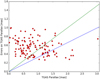 |
Fig. 1 Error on the parallax σϖ as a function of the parallax ϖ for the 124 S stars resulting from the intersection of the General Catalog of Galactic S stars (Stephenson 1984) and Gaia DR1 (Gaia Collaboration 2016), observable with the HERMES spectrograph (δ > −30°). The blue and green lines delineate the quality conditions defined as σϖ = 0.3 ϖ and σϖ = 0.5 ϖ, respectively. |
2 Observations and target selection
2.1 S stars from the Gaia catalogues
Among the 1347 S stars of the General Catalog of S stars (GCSS Second Edition; Stephenson 1984), 321 are present in the Gaia Data Release 1 (DR1; Gaia Collaboration 2016), made available when the present study started. If we consider only targets observable from the Roque de los Muchachos Observatory (La Palma, Canary Islands, and thus eligible for a HERMES high-resolution spectrum), that is, with δ > −30°, the intersection reduces to 124 objects (see also Sect. 2.2).
The (ϖ, σϖ) plane (where ϖ is the DR1 parallax andσϖ its error) for these 124 S stars is presented in Fig. 1. For the present study, only stars with good-quality DR1 parallaxes are selected, that is, matching the condition σϖ ∕ϖ ≤ 0.3. This condition ensures that the distance obtained by simple inversion of the parallax is not significantly biased. The positioning of individual stars on specific evolutionary tracks, as performed in Sect. 6, indeed requires accurate distance estimates. These 18 S stars with Gaia DR1 parallaxes are located below the blue line in Fig. 1. Our final sample of 19 S stars includes as well UY Cen, which is not observable with HERMES but has a UVES spectrum and satisfies the condition on ϖ∕σϖ. The list of the 19 target S stars is presented in Table 1. Although the sample selection for the present investigation is, as described above, based on Gaia DR1, during the course of our study the DR2 parallaxes were released. We used these more accurate parallaxes, listed in Table 1, for the present paper. Our study was not extended to the full DR2 sample of S stars with accurate parallaxes, though, since we had not collected high-resolution spectra for all of them. The full GDR2 S-star sample analysis is therefore deferred to a forthcoming paper. Table 1 shows that distances obtained by simple inversion of the parallaxes are compatible within 1σ with the Bayesian estimate provided by Bailer-Jones et al. (2018). In the remainder of the paper, we will thus use distances obtained from a simple inversion of the parallax.
In fact, many bright stars with G ≤ 7 (where G is the Gaia magnitude) and “extremely blue and red sources” are missing from the Gaia DR1 (Gaia Collaboration 2016). The red cut introduces a bias against intrinsic S stars in our sample as intrinsic S stars are redder, on average, than extrinsic S stars:  as compared to
  (Van Eck et al. 2000). Therefore, many among the most evolved (intrinsic) S stars are absent from our sample.
Basic data for the S star targets.
2.2 High-resolution spectra
The availability of HERMES1 high-resolution spectra (Raskin et al. 2011) is needed to derive accurate atmospheric parameters of S stars. The HERMES spectrograph is mounted on the 1.2m Mercator Telescope at the Roque de Los Muchachos Observatory, La Palma (Canary Islands). It is a fibre-fed spectrograph in a temperature-controlled environment which ensures good wavelength stability. HERMES spectra have a wavelength coverage of 380–900 nm with a spectral resolution of R = 85 000. The spectra are automatically reduced through a dedicated pipeline at the end of the observing night.
The 18 S-type stars matching the conditions mentioned in Sect. 2.1 all have V < 11, and are thus easily observable with HERMES. The observation log is given in Table 2. The spectrum of one additional intrinsic S star, UY Cen, was obtained from the UVES POP database2 (Bagnulo et al. 2003). The TGAS parallax of UY Cen satisfies the parallax condition (Sect. 2.1) but with a declination δ = −44°, it is not observable with HERMES. UY Cen is an interesting benchmark star already studied in SVE17.
2.3 Classification based on Tc lines
A S/N ratio larger or equal to 30 in the V band is needed to detect Tc lines in S stars spectra (Van Eck et al. 1998). For this purpose, we use the three strong Tc I resonance lines locatedat 4238.19, 4262.27 and 4297.06 Å. As mentioned by Little-Marenin & Little (1979) and Van Eck & Jorissen (1999), all three lines are severely blended but can nevertheless be used to distinguish intrinsic from extrinsic S stars. We classified 16 stars as Tc-poor (Fig. 2) and 3 stars as Tc-rich (Fig. 3), namely NQ Pup, V915 Aql and UY Cen. There is a good correlation between the diagnostics provided by the 4238.19 and 4262.27 Å features. Because the 4297.06 Å Tc line is blended by other s-process element lines (especially by Nb), even when the star is devoid of Tc, the strength of that feature varies from one Tc-poor star to another (see Fig. 2), depending on the average s-process overabundance.
UY Cen is an ambiguous case. It shows a clear absorption feature at 4238.19 and 4297.06 Å, thus hinting at its Tc-rich nature, but the absorption feature is not as clear at 4262.27 Å (a fact also reported by Van Eck & Jorissen 1999). Based on the two lines providing consistent results, we classify UY Cen as Tc-rich; this classification is further supported by its infrared excess (Sect. 7 and Fig. 19).
The presence of Tc was first detected in V915 Aql by Little et al. (1987), and Fig. 3 clearly confirms the Tc-rich nature of that star. NQ Pup was classified as intrinsic S star by Smith & Lambert (1988); we confirm this classification, as we do for the Tc-poor nature of HD 189581, HD 191589, HD 191226, HD 150922 and HD 215336 as previously found by Smith & Lambert (1988) and of BD −28°4592 and V1135 Tau as formely published in Jorissen et al. (1993). Wang & Chen (2002) classified HD 233158 and BD −10°1977 as Tc-deficient from their location in the (K − [12]) − ([12] − [25]) photometric plane. Finally, Otto et al. (2011) found BD +69°524 to be Tc-poor from the IRAS photometry. We confirm these results from the analysis of our high-resolution spectra (Fig. 2).
For some objects however there are some disagreements with previous assignments. V530 Lyr was classified as Tc-rich by Smith & Lambert (1988) and Van Eck et al. (1998), but they mention that their classification for this star was uncertain due to the blend at 4262.27 Å. Similarly, HD 63733 was classified as Tc-rich by Smith & Lambert (1988) and Van Eck et al. (1998), though the latter mentioned an uncertainty on this classification. However, from the features at 4238.19 and 4262.27 Å, we re-classify unambiguously both stars as Tc-poor.
Finally, there was no former classification available for AB Col, TYC 5971-534-1, FX CMa and BD −22°1742 in the literature. From their Tc features (Fig. 2), we have tagged all four stars as extrinsic S stars. The final Tc-rich/poor assignment for our sample stars is listed in Table 4.
To confirm the paradigm that Tc-deficient S stars are always member of binary systems, we investigated the binary status of our extrinsic S stars. HD 63733, HD 189581, HD 191226, HD 191589, HD 215336, V530 Lyr, BD +28°4592, and V1135 Tau are known to be binary systems (Jorissen & Mayor 1988; Brown et al. 1990; Jorissen et al. 1993). The radial velocity (RV) for the other extrinsic S stars was not monitored to check their binarity.
Similarly, for the three intrinsic S stars, there is no RV monitoring available to test their binarity. However, the frequency of occurrence of binary systems among intrinsic S star is expected to be similar to that among normal (that is, non s-process-enriched) stars. For a discussion of this topic, see for example Table 9.1 and Sect. 9.3 in Jorissen (2004) as well as Jorissen et al. (1993). We note that Brown et al. (1990) classified NQ Pup and V915 Aql as single stars from the absence of the He I features at 10 830 Å, contrary to the situation prevailing for binary systems with a white dwarf companion where this feature is observed.
List of S stars with available TGAS solution and high-resolution spectra.
3 Stellar parameters determination
In an attempt to obtain the stellar parameters for S-type stars solely based on photometric data, we designed a spectral energy distribution (SED) fitting routine called S4U (S stars SED fitting Utility). SED fitting has been used as a successful technique for atmospheric parameter determination of barium (Escorza et al. 2017) and post-AGB stars (Hillen et al. 2017). Hence, we tested the capability of photometric observations alone to constrain the extended parameter space of S-type stars with S4U (Sect. 3.1). Because photometry alone cannot lift the degeneracies between the S star stellar parameters, we later developed a second method (Sect. 3.2) based on comparing a high-resolution HERMES spectrum with the grid of synthetic spectra from SVE17. We shall confirm, as already mentioned by SVE17, that high-resolution spectroscopy is needed for the careful disentanglement of the atmospheric parameters of S stars.
3.1 S4U: S stars SED Fitting Utility
The S4U code compares the available photometric observations of a given star with those computed from the synthetic spectra of the grid of S-star models (SVE17). S4U is an extension of the tool described in Degroote et al. (2011) for the SED fitting with Kurucz atmospheric models. The five dimensions of the S4U parameter space are Teff, log g, reddening EB−V, [C/Fe], and [s/Fe]. The inclusion of [C/Fe] and [s/Fe], which are atmospheric parameters important for S stars (SVE17 and Sect. 1), makes S4U a specific tool for SED fitting of S stars.
3.1.1 Method
S4U collects first the photometry of the targets from the SIMBAD database (Wenger et al. 2000). These photometric data are carefully cleaned, removing all the saturated data points as well as those flagged as unreliable sources by SIMBAD. S4U cannot be used for large-amplitude pulsators like Mira variables since the photometric data were most likely collected at different epochs. S4U uses 2 grids of model SEDs, separately for metallicities [Fe/H] = 0.0and −0.5. These model SEDs are medium-resolution synthetic spectra computed from the MARCS model atmospheres of the S-star grid. The parameter range covered by this grid is 2700–4000 K (with steps of 100 K) for Teff, 0 ≤ logg ≤ 5 (with steps of 1 dex), C/O from 0.5 to 0.99 (0.50, 0.75, 0.90, 0.92, 0.95, 0.97, 0.99), [s/Fe] of 0.0, +1.0, +2.0 dex, and [α/Fe] scaled with metallicity. The microturbulence is fixed at 2 km s−1. Next, a photometric grid is obtained by integrating each synthetic spectrum of the model grid over the transmission curves of the various photometric filters. The photometric systems used by S4U include HIPPARCOS, Strömgren, Johnson, Cousins, 2MASS, Geneva, Tycho2, Galex, DENIS, SDSS and USNO-B. The photometry has been calibrated using the Vega model of Bohlin & Gilliland (2004) with the zero points of Maíz Apellániz (2007).
Only photometric bands bluer than K are considered for the SED fitting, to avoid being sensitive to possible photometric excesses caused by circumstellar dust. A χ2 statistics is then used to establish the goodness-of-fit for about 1 million models obtained randomly by interpolation of the photometric grid in the five atmospheric parameters listed above. The best-fitting model is of course the one with the minimum χ2. The error on the parameters is derived as the 1-σ error enclosing 67% of the model fits (see the coloured regions of Fig. 4b–d).
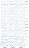 |
Fig. 2 The spectral region around the three (4238.19, 4262.27 and 4297.06 Å) ultra-violet Tc I lines in Tc-poor S stars. The observed spectra have been normalized using unity-based normalization. |
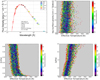 |
Fig. 4 Top left panel: SED fitting of V915 Aql using S4U where the red line represents the MARCS model best matching the photometric observations collected from SIMBAD. Top right panel: probability distribution plot of log g vs Teff for V915 Aql obtained using S4U. Bottom left panel: same as top right panel but for [C/Fe] vs Teff and bottom rightpanel for [s/Fe] vs Teff. The red plus sign in top right, bottom left and right panels indicates the best model selected by S4U. |
3.1.2 Discussion
Obtaining the stellar parameters for S-type stars from SED fitting with photometry alone turns out to be very challenging. This is due to the coupling between Teff, [C/Fe], and [s/Fe], and to the fact that the latter two values cannot be constrained solely by broadband photometry. The SED fitting (top left panel of Fig. 4) and the plots of reduced probability (top right, bottom left, and right panels of Fig. 4) provide a visual demonstration of the above conclusion.
The distribution of reduced probability in the logg – Teff plot (top right panel of Fig. 4) shows that S4U constrains Teff reasonably well, since a vertical strip of dark colours (low reduced probabilities imply low χ2 values and hence best-fitting models) is well visible. The width of this strip of dark-coloured points shows that Teff is constrained within 200 K for V915 Aql. To broaden the quality check, we compared as well the S4U atmospheric parameters with those obtained by SVE173 (Table 3). It appears that S4U reproduces the SVE17 Teff within 200 K, as expected from the above-mentioned error bar.
On the contrary, logg appears to be highly contingent upon the available photometric bands. As explained by SVE17, good constraints on log g are provided by blue, violet, and ultraviolet filters. The poorly constrained S4U log g value for V915 Aql is apparent from Fig. 4, since the dark strip of well-fitting models spans the complete range on the y-axis.
To avoid the degeneracy due to the sensitivity on the available photometric filters and to prevent S4U from converging to large and unphysical logg values of 3–5 (typical of dwarf and sub-giant stars), we restricted the log g range available to S4U to 0–1 dex. This is the typical range of logg obtained by SVE17 for their sample of 66 Henize S stars (Table 3), among which no dwarf star was uncovered.
The C/O is a parameter of paramount importance for S-type star atmospheres. It is severely dependent on the adopted effective temperature and plays a major role in fixing the TiO and ZrO band strengths in S stars. However, the broadband photometry used by S4U is quite insensitive to these band strengths. This might explain why the S4U estimates of [C/Fe] and [s/Fe] are strongly discrepant with respect to those obtained by SVE17 (Table 3). Therefore, S4U cannot constrain the C/O (or [C/Fe]), and this is apparent in the bottom left panel of Fig. 4. The situation is similar for [s/Fe], as shown by the bottom right panel of Fig. 4 in the case of V915 Aql. This holds true for other S stars as well (Table 3).
To conclude, a SED fitting tool like S4U based solely on broadband photometry delivers a quick initial estimate of Teff, but is unable to reliably constrain logg, [C/Fe], and [s/Fe]. Nevertheless, the interest of this photometric attempt at determining atmospheric parameters of S-type stars is to underline the difficulties specific to this class of peculiar red giants. They call for a more sophisticated method involving high-resolution spectroscopy, as described in the next section.
Stellar parameters for a set of Henize stars obtained from SVE17, compared with results from S4U.
3.2 Atmospheric parameters derived from spectral fitting
Realizing the limitations of S4U, we devised a spectral-fitting method4 that is more efficient at disentangling the atmospheric parameters of S stars. The method is very similar to that described in Neyskens et al. (2015) and SVE17, and searches for the best-fitting MARCS model by comparing the associated synthetic spectra with chunks of the observed spectrum, along with a couple of photometric indices.
Since the observed high-resolution spectra are not flux-calibrated, the slope of the spectrum is not reliable over extended wavelength regions (≥100 Å). It is therefore necessary to compare the synthetic and observed spectra over small spectral domains (about 100 Å) that have been normalized by matching the points of maximum flux, and this is done separately within each considered chunk.
The high-resolution synthetic spectra are generated by the Turbospectrum radiative-transfer code (Alvarez & Plez 1998, Plez 2012) using the MARCS model atmospheres from SVE17. The synthetic spectra have been convolved with a Gaussian kernel to a resolution matching that of the observed spectrum and reddened to match the reddening of the target star, as derived from the Gontcharov (2012) table with the distance computed from the DR2 parallax. The comparison between observed and synthetic spectra is then performed through χ2 -minimization, summing over all spectral pixels, and using the flux itself as an estimate of the variance on the observed spectrum. In this process, it is important to remove spectral regions contaminated by telluric lines, as well as strong lines like the Na D doublet, whose core flux is close to zero in the observed spectrum. Since the core of the line is not well reproduced in the synthetic spectrum, it would lead to very large spurious contributions to the χ2 value if it were not discarded.
The dereddened V –K and J–K photometricindices have been used as well in the comparison. They have been attributed arbitrary weights corresponding to 20 000 pixels, so that they contribute to the χ2 in proportion to their band width. The adopted 1σ error were 0.04 and 0.01 for V − K and J− K, respectively. Values of χ2 for every spectral chunk and photometric indices are then calculated.
The model with the lowest total χ2 value is then selected as the best-fitting model, providing a first estimate of atmospheric parameters. Finally, we validate the stellar parameters by checking high-resolution spectral windows (for example, the 50 Å spectral window including the two λ7819 and λ7849 Å Zr lines; see Figs. 8 and 9).
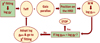 |
Fig. 5 Iterating scheme to constrain logg. |
3.3 Constraining log g with DR2 parallaxes
To better constrain the gravities derived from the spectral-fitting method, spectral chunks in the U band would be required (see the discussion in SVE17). However, these red stars have weak signals in that spectral range. Here we use instead the star location in the HR diagram (see Sect. 6) to constrain its mass and radius, and hence its gravity that we name “Gaia log g” in the following. This Gaia logg is derived from the relation:
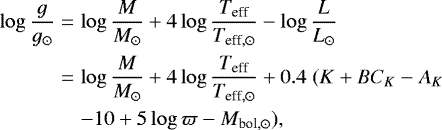
where ϖ is the Gaia DR2 parallax expressed in mas; AK is the extinction in the K band, derived as described in Sect. 3.2; Teff and BCK, the bolometric correction in the K band, are taken from the MARCS model with the lowest χ2. The mass is determined by selecting the evolutionary track of the corresponding metallicity passing closest to the star location in the HR diagram (details about the stellar models are provided in Sect. 5.1). Since the Gaia log g obtained in this way generally does not match the one from the spectral-fitting tool, the process was iterated as illustrated in Fig. 5.
In the next iteration, we thus adopted the new Gaia log g and chose the first model in the list of best-fitting models having logg matching the Gaia logg value. With this new model (which could have a Teff and/or metallicity which differ from the previous one), we obtain a new position in the HR diagram. This iterative process is pursued until it converges towards a consistent logg value.
3.4 Uncertainties on the atmospheric parameters
As explained above, finding the atmospheric parameters (Teff, log g, [Fe/H], C/Oand to a lesser extent [s/Fe]) for S stars is an intricate process, and so is the estimate of their uncertainties. The methodwe followed is inspired by that of Cayrel et al. (2004). It consists in finding alternate atmospheric parameters which lead to an acceptable fit of the high-resolution spectrum. We illustrate the procedure with V915 Aql. Its best parameters are Teff = 3400 K, log g = 0, [Fe/H] = − 0.5, C/O = 0.75, and [s/Fe] = 0 dex (Table 4). In the following, this set of parameters will be called “model A”. In the list of best models provided by the χ2 method, one of the models coming after A has Teff = 3500 K, logg = 1, [Fe/H] = 0.0, C/O = 0.5, and [s/Fe] = 1 dex. We denote this as “model H”. Figure 10 reveals that the synthetic spectrum for model H fits the Zr I 7819 Å line almost equally well as the spectral fit for model A, though model A and model H differ from each other by one grid step for each of their parameters. We therefore consider that one grid step in each of the considered parameters represents a fair estimate of their uncertainty (and consequently, that an interpolation in the model grid would not provide any accuracy improvement). An estimate of the impact of these model-parameter uncertainties on the s-process abundance uncertainty will be discussed in Sect. 4.4.
4 Abundance determination
The abundances for all the considered elements were derived by comparing the observed spectra with synthetic spectra generated by Turbospectrum using MARCS model atmospheres. We have used the same molecular and atomic line lists as SVE17.
4.1 C, N, O
The spectra of S stars are dominated by oxygen-bearing molecular bands. An accurate estimate of the C, N, and O abundances is needed as a prior to derive accurate atomic abundances. The carbon abundance is determined from sensitive features in the CH band around 4300 Å (Fig. 6). Because the λ 6300.3 Å [O I] line lies in aseverely blended region, it is not possible to use it for deriving the O abundance. Therefore, we use instead a metallicity-scaled solar O abundance value throughout our study. The C/O was varied over the whole range 0.50–0.99 and synthetic spectra withthose values were compared to the observed spectrum in order to confirm that the spectral-fitting routine indeed provides the most appropriate C/O. Since we derived the carbon abundance from the CH G-band and the C/O from an overall spectral fit, we may combine these values to derive the oxygen abundance. We checked that it was indeed consistent with the assumed metallicity-scaled solar O abundance. We found an agreement better than 0.2 dex in all our stars, except for TYC 5971-534-1, for which the discrepancy in logϵO amounts to 0.26 dex.
The uncertainty on C/O was estimated from the values of the C/O providing an acceptable fit to the CH G-band.
The nitrogen abundance was then derived from the CN lines available in the 7900–8100 Å range (Fig. 7), using in particular the lines listed in Merle et al. (2016). We note, however, that for stars with C/O ≳0.9, the CN lines are strong and their sensitivity to the N abundance is therefore limited, making the N abundance uncertain.
4.2 Metallicity [Fe/H]
Metallicity is derived from Fe line synthesis (in the range λ7300–λ8700 Å). Metallicities along with the number of lines used and their standard deviations are listed in Table 4; the full line list is given in Sect. A.1.
Atmospheric parameters for S stars after performing iterations on log g.
4.3 s-process elements
Abundances of Zr and Nb are derived for all our programme stars (Tables 5 and 6). The Zr abundances were measured from the two Zr I lines with transition probabilities from laboratory measurements (Biémont et al. 1981) at 7819.37 and 7849.36 Å (see Figs. 8 and 9). As discussed by Neyskens et al. (2015) and Karinkuzhi et al. (2018), the above Zr I lines systematically lead to Zr I abundances 0.30 dex lower than abundances derived from lines with transition probabilities from Corliss & Bozman (1962). We favour the former lines as they rely on measured transition probabilities.
The Nb abundances for our stars were estimated from the Nb lines listed in Table A.1. Not all Nb lines which are listed in Table A.1 were present in all stars, though, and finding good Nb lines for the intrinsic S stars was even more challenging because of the strong molecular blending. We did not derive the Nb abundance for the intrinsic S star UY Cen as we could not find any well-reproduced Nb line or blend. On average, we used four Nb lines for every extrinsic S star and two for intrinsic S stars. These Zr–Nb abundances will be discussed in Sect. 5.4.
In addition to Zr and Nb, we attempted to determine Sr, Y, Ba, La, Ce, Nd, Sm and Eu abundances in the intrinsic S stars of our sample (Table 6). Finding good Sr lines was impossible for NQ Pup and V915 Aql, and we could derive the Sr abundance for UY Cen using only one Sr line. We could find two good Y lines in UY Cen and even more in NQ Pup and V915 Aql. The Ba abundance was derived using only one Ba line at 7488.077 Å since other Ba lines were heavily saturated. The La abundance was derived for NQ Pup and UY Cen but not for V915 Aql. The Ce and Nd abundances were derived using at least two lines for all three stars. The Sm abundance could be derived only for UY Cen and NQ Pup. The Eu abundance could only be obtained for NQ Pup from one Eu line. All the atomic lines used for the abundance determination are listed in Table A.1 with their excitation potential and log gf.
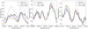 |
Fig. 6 Carbon abundance derived from a comparison between the observed spectrum of the extrinsic S star HD 189581 in the CH G-band (black line) and the synthetic spectrum for different C/O values. The best agreement is obtained for C/O = 0.5. The grey line presents the synthesis without the CH linelist. |
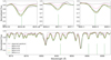 |
Fig. 7 Bottom panel: comparison between the synthetic and observed spectra for V530 Lyr in the 8076–8088 Å range containing CN lines. Top three panels: ±1 Å zoom around the CN lines at 8035, 8057.3, and 8082.9 Å (from left to right panels). The green dashed lines mark the CN lines used by Merle et al. (2016) in barium stars. The grey line presents the synthesis without the CN line list. The value [N/Fe] = 0.9 has been adopted. |
4.4 Uncertainties on the abundances
The s-process abundance uncertainties were estimated for the three intrinsic S stars NQ Pup, V915 Aql and UY Cen, because they cover an effective temperature range (3300–3700 K) representative of that of S stars, and becausethe spectra of intrinsic S stars are often more blended than those of extrinsic S stars, so the errors can only be overestimated when applied to our entire sample. Uncertainties are listed in the bottom panels of Tables 7–9. In the upper panels, model A designates the adopted model, whereas models B–G correspond to models differing by one grid step from model A, each parameter varied at a time. The abundance resulting from each of these models is then compared with the abundance from model A and these differences are listed as columns Δ B−A,..., ΔG−A in the bottom panels of Tables 7–9.
The stellar parameters of S stars are strongly correlated to one another. Hence, the total error budget should account for this entanglement between the stellar parameters. We followed a method similar to that of Cayrel et al. (2004) to estimate the uncertainties on our abundances due to the entangled stellar parameters. After modifying Teff by +100 K or −100 K from model A, we adjusted the other stellar parameters to obtain an acceptable fit to the global spectrum, as already explained in Sect. 3.4. We designate this alternate model as “H” in Tables 7–9.
To further illustrate the strong coupling between atmospheric parameters in S-type stars, Fig. 10 compares synthetic spectra around the Zr I 7819 Å line for models A and H of V915 Aql. While there are significant differences between the parameters of the two models (|ΔTeff| = 100 K, |Δlogg| = 1, |Δ [Fe/H]| = 0.5, |Δ C/O| = 0.25, |Δ [s/Fe]| = 1), it is extremely difficult to decide which model has to be preferred from this plot alone. This reveals an intrinsic uncertainty existing for S-star atmospheric parameters. However, our technique consisting in a global assessment combining a χ2 minimization with gravity determined from the Gaia parallax can help to solve this puzzle. Indeed, the log g value associated with model H for V915 Aql and UY Cen is incompatible with the “Gaia log g”. Furthermore, for V915 Aql, model H is inconsistent with the derived s-process overabundance: model H has [s/Fe] = +1 dex, whereas the individual abundances do not exceed 0.5 dex. Both arguments support the selection of model A over model H.
For NQ Pup, the situation is more tricky, models A and H only differing by |Δ Teff| = 100 K and |Δ C/O| = 0.25. However, the comparison of the spectral fit in the TiO bands for models A and H clearly favours model A (Fig. 11).
The expected uncertainty on the abundances due to the changes of multiple stellar-parameter (Col. Δ H−A of Tables 7–9) is estimated as the difference between the abundances derived from models H and A (the reference model).
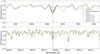 |
Fig. 8 Illustration of the quality of the match between observed and synthetic spectra obtained for the extrinsic S star V530 Lyr around the Zr line at 7849.37 Å. The upper panel presents a ± 3Å zoom. |
4.5 Abundance profiles of the three intrinsic S stars NQ Pup, UY Cen, and V915 Aql
As a star evolves on the AGB, it is subject to several episodes of third dredge-up resulting into progressive surface enrichment of carbon and s-process elements. The direct monitoring of this evolution of abundances along the AGB requires to consider stars of similar masses and metallicities. Unfortunately, as we will show in Sect. 6, the three intrinsic S stars of our sample lie on evolutionary tracks of different masses (MNQ Pup ~ 2.5 M⊙, MUY Cen ~ 3 M⊙, MV915 Aql ~ 1 M⊙), even though NQ Pup and UY Cen have similar metallicities ([Fe/H] approximately ~ −0.3) close to that of V915 Aql ([Fe/H] approximately −0.5). Therefore, the expected correlation between the evolutionary stage and the overabundance level cannot be readily investigated, even though UY Cen has the largest s-process enrichment and is more evolved on the AGB as compared to NQ Pup.
We present the abundances of these three intrinsic S stars in Table 6, and discuss them in turn in the remainder of this section.
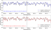 |
Fig. 10 Comparison between the observed spectrum of V915 Aql (black line) and synthetic spectra corresponding to model A (top panel, blue line) and to model H (bottom panel, red line), in the region surrounding the Zr I λ7819 Å line. |
C, N, Zr, and Nb abundances in extrinsic S stars.
4.5.1 NQPup
Our Teff, log g and [Fe/H] values match well with those of de Boer & Cottrell (2009), but their C/O > 1 is larger than our estimate of C/O = 0.5, which is in agreement with that of Neyskens et al. (2015). Our metallicity is also very similar to that of Neyskens et al. (2015; [Fe/H] = −0.30 and −0.31, respectively).
The s-process abundance profile of NQ Pup (left row of Fig. 12) reveals a mild enhancement in s-process elements (and even no detectable Ce enhancement), well in line with the nearly solar C/O. Our La II, Nd II, and Eu II abundances agree with those from de Boer & Cottrell (2009) within error bars. We report lower [Y/Fe] and [Zr/Fe] values as compared to de Boer & Cottrell (2009). Our Zr abundance differs by 0.17 dex from that of Neyskens et al. (2015) despite the fact that the same Zr lines have been used in both studies. Our effective temperature differs by 200 K, but the sensitivity of the Zr abundance on Teff is too weak to fully account for the observed difference (Table 7). The abundance difference is thus probably due to differences in the continuum placement.
4.5.2 V915 Aql
No chemical abundances were reported so far for this Tc-rich S star. Though the carbon content in V915 Aql (C/O = 0.75) is slightly higher than in NQ Pup, we do not measure a stronger s-process enrichment. From the middle panel of Fig. 12, we see that the light and heavy s-process elements reach similar overabundance levels in both stars. We confirm that we do observe indications of a moderate s-process overabundance in V915 Aql, including the presence of Tc. Given its low-mass (1 M⊙) inferred from its location in the HR diagram (Fig. 16), this conclusion is of importance in the framework of stellar evolution, as we will further discuss in Sect. 5.
As for NQ Pup, uncertainties on Teff have the strongest impact on the abundance determination.
Elemental abundances for NQ Pup, UY Cen, and V915 Aql, along with the standard deviation due to line-to-line scatter.
4.5.3 UY Cen
Abundance determination in UY Cen is a challenging task because of its low temperature and C/O close to unity. It is consequently an SC star (consistent with its S6/8 spectral type). Abundance analyses of stars of that kind are known to be challenging (Catchpole 1982, SVE17). The gaps present in the UVES spectral coverage even strengthen the challenge. The elemental abundances were derived from few lines only and to vindicate our results, we compared them with the abundances from Catchpole (1982), keeping in mind however that SC-like atmospheric models were not available at the time. Catchpole reported that all elements heavier than Fe are overabundant by 0.6 dex in UY Cen. We observe a similar overabundance level (right panel of Fig. 12). Catchpole scaled his abundances with respect to Ti and obtained [Ti/H] = −1.05 and [Fe/Ti] = 0.3 which results in [Fe/H] = −0.75. On the contrary, we derive a metallicity [Fe/H] = −0.3. This result is obtained from a selection of very good non-blended and non-saturated Fe lines.
Most s-process elements are highly enriched in UY Cen with [X/Fe] > 1, in particular Sr, Y, Zr, La, and Nd. UY Cen is significantly more s-process enriched than NQ Pup (Fig. 12). This isconsistent with the positions of these two stars in the HR diagram where UY Cen appears more evolved on the TP-AGB (middle panel of Fig. 16), though on an evolutionary track with a higher mass.
5 Comparison of abundances with nucleosynthesis predictions
5.1 Stellar models and nucleosynthesis calculations
To locate the stars in the HR diagram, evolutionary tracks have been computed with the STAREVOL code whose detailed description can be found in Siess et al. (2000) and Siess & Arnould (2008). In short, this code considers the radiative opacity tables of Iglesias & Rogers (1996) above 8000 K and of Ferguson et al. (2005) at lower temperatures. Opacity enhancement due to the formation of molecules in carbon-rich atmospheres is also accounted for following the formulation of Marigo (2002). The Schröder & Cuntz (2007) prescription for the mass-loss rate is considered up to the beginning of the AGB phase and then the Vassiliadis & Wood (1993) formulation is applied. To follow the abundances of heavy elements, we use a nuclear network of 411 species with all the relevant reactions for the s-process nucleosynthesis. We adopt the solar abundance distribution of Asplund et al. (2005) and consider overshooting below the envelope at all times. A diffusion equation is used to simulate the partial mixing of protons in the C-rich layers at the time of the third dredge-up. Following the formalism of Eq. (9) of Goriely & Siess (2018), the diffusive mixing (DM) parameters adopted in our calculations are Dmin = 109 cm2 s−1 and p = 5, where Dmin is the value of the diffusion coefficient at the innermost boundary of the diffusive region and p is an additional free parameter defining the slope of the exponential decrease of the overshoot diffusion coefficient with depth.
5.2 The s-process abundance distribution
The observed abundance profiles of the 3 intrinsic S stars have been compared with nucleosynthesis predictions from the STAREVOL code. The surface abundance distribution displayed in the right panels of Fig. 13 corresponds to the outcome of s-process nucleosynthesis in an AGB model with the same metallicity as the target star (as listed in Table 6), and a mass matching the star location in the HR diagram (left panels of Fig. 13). The listed mass and pulse number are indicative. The pulse number is chosen in order to optimally match both the overabundance level and the location in the HR diagram. Although such an agreement is not guaranteed a priori, it is reached at least for NQ Pup. For that star, there is a good match between models and observations not only for luminosities and temperatures, but also for most abundances (except Ce and Eu).
The case of V915 Aql is more puzzling (middle panel of Fig. 13), since the star lies at an uncomfortably low mass and luminosity for the third dredge-up to occur. This object would require a 1 M⊙ model to match its location in the HR diagram, but no s-process surface enrichment is predicted at such a mass because models do not predict the TDU to operate for M ≲ 1.3 M⊙ (e.g. Karakas & Lugaro 2016, and the present STAREVOL models). To account for V915 Aql surface abundances, a 1.5 M⊙ model had to be used, but such a model does not agree with the position of V915 Aql in the HR diagram. Nevertheless, abundance predictions for this model reproduce fairly well the overabundance pattern of V915 Aql (except for La).
Finally, concerning UY Cen (bottom panel of Fig. 13), a 3.5 or 4 M⊙ model would be needed to match its location in the HR diagram. However, such high-mass models do not succeed in matching the rather high level of measured overabundances, because the large envelope mass leads to a strong dilution. A 3 M⊙ stellar model allows a better match of the abundances, but in turn is too faint to match UY Cen luminosity in the HR diagram.
Sensitivity of the elemental abundances of NQ Pup upon variations of the atmospheric parameters.
5.3 Comparison between the modelled and measured carbon and s-process enrichments
The sensitivity of the s-process abundances to the pulse number may be assessed from Fig. 14, which displays the evolution of the Zr and La abundances as a function of the pulse number for the two intrinsic stars with best-matching evolutionary tracks in the HR diagram, namely, NQ Pup and UY Cen. For NQ Pup, constraints from Zr and La appear to be mutually compatible with the C/O evolution, pointing at pulse numbers in the range 5–8. For UY Cen however, the measured La and Zr abundances are difficult to reconcile with the model C/O, which increases too rapidly to remain in the range of values characterizing S stars (0.5 < C∕O < 1). Thus, models do not seem to correctly predict the respective rates at which the s-process and carbon abundances increase as a function of pulse number. If such a mismatch occurs at a later evolutionary stage along the TP-AGB, it will be far better noticeable as the discrepancy increases with pulse number (compare for example the cases UY Cen and NQ Pup).
This discrepancy between s-process and C enrichment levels was already outlined by Goriely & Mowlavi (2000). From their Figs. 12 and 13, it can be inferred that a C/O of unity (which corresponds to the upper limit for an S-type star) implies [Zr/Ti] in the range 0.5–0.8 which is less than the value of [Zr/Fe] = 1.0 estimated for the SC star UY Cen.
For some objects however, the discrepancy goes in the opposite direction: in the metal-poor ([Fe/H] = −2.2) post-AGB star V453 Oph, Deroo et al. (2005) found a moderate s-process enrichment ([s/Fe] ~ 0.5) not accompanied by a simultaneous C-enrichment. The observed upper limit on the nitrogen abundance in this object excluded a possible CN-cycle destruction of the dredged-up carbon. Moreover, the abundances of elements of similar condensation temperatures as carbon proved that the atmosphere was not depleted in refractory elements like carbon (such a depletion pattern is indeed typical in binary post-AGB stars). We must thus conclude that a key piece is missing for a successful modelling of the simultaneous s-process and carbon enrichments in AGB and related stars of various metallicities.
A possibly related issue is the marked gap between the (modest) C and s-process enhancements observed in (N-type) carbon stars and those observed in post-AGB stars (De Smedt et al. 2015).
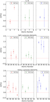 |
Fig. 12 Abundances of the three intrinsic S stars, with C and N (top panel), light s-process elements (middle panel) and heavy s-process elements (bottom panel). The error bars on the elemental abundances represent the total uncertainty calculated by quadratically summing the Δ H−A values from the last columns of Tables 7–9 with the standard deviation due to line-to-line scatter, plusan extra 0.1 dex as uncertainty due to continuum placement. |
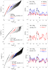 |
Fig. 13 Left panels: location of the three intrinsic S stars in the HR diagram, compared with STAREVOL tracks of the corresponding metallicity. Right panels: predicted abundance distribution of the three intrinsic S stars. Top panels: NQ Pup, centralpanels: V915 Aql, and bottom panels: UY Cen. |
5.4 The Zr–Nb pair
In extrinsic S stars, the time elapsed since the end of the mass-transfer episode is sufficient for 93Zr to have fully decayed into mono-isotopic Nb. Actually, mono-isotopic Nb can only be produced byβ-decay of 93 Zr (half-life of 1.53 × 10⁶ yr). Hence, extrinsic stars should be enhanced in niobium as compared to intrinsic stars. The Zr–Nb pair may therefore be used to confirm the Tc-rich/Tc-poor dichotomy (see the more extensive discussion by Neyskens et al. 2015 and Karinkuzhi et al. 2018). Figure 15 shows the trend of [Zr/Fe] vs. [Nb/Fe] for the intrinsic and extrinsic S stars of our sample. There is indeed a clear difference between the positions of intrinsic S stars and extrinsic (barium and S) stars in this plane. The two intrinsic, Tc-rich S stars (NQ Pup and V915 Aql) are, as expected, Nb-poor, and their Nb and Zr abundances are in excellent agreement with those predicted by AGB nucleosynthesis in 2 or 3 M⊙ stars.
We nowcompare in this diagram the location of extrinsic S stars with that of barium stars. Despite their larger error bars (due to the cooler, more blended spectra of S stars), the Nb and Zr abundances of extrinsic S stars are well in line with those of barium stars, as expected since extrinsic S stars are just the cooler analogs of barium stars (see Fig. 17 below). The fact that Nb and Zr abundances of most barium stars in Fig. 15 are larger than those of extrinsic S stars is probably due to a selection bias, since Karinkuzhi et al. (2018) deliberately selected highly enriched barium stars (so that their primordial Nb and Zr abundances could be neglected).
6 The HR diagram of S stars
Figure 16 presents the HR diagram of our sample of S stars using the final stellar parameters from Table 4 and the stellar evolutionary tracks of the corresponding metallicity computed with the STAREVOL code. The asymmetric error on luminosities was derived by propagating the symmetric error on the parallax.
The derivation of stellar masses is possible by locating individual stars on evolutionary tracks of the corresponding metallicity. Both metallicity and mass are listed in Table 4. Although no uncertainty on the mass is given in Table 4, it may be estimated from Fig. 16 by noting that the main sources of uncertainty are the ± 100 K uncertainty on the Teff derivation, along with an intrinsic error of about 100–150 K on the location of the evolutionary tracks themselves (Cassisi 2017).
The twointrinsic stars NQ Pup and UY Cen are both located on the TP-AGB, as expected. UY Cen is located well above the predicted onset of TDU (black dotted line in the middle panel of Fig. 16, corresponding to the lowest stellar luminosity following the first occurrence of a TDU episode), which is consistent with its large overabundance level in s-process elements. On the contrary, NQ Pup lies just above the TDU threshold, as already reported by Van Eck et al. (1998).
The intrinsic (Tc-rich) S star V915 Aql, with [Fe/H] = −0.5 and located along a 1 M⊙ track, constitutes a most puzzling case (as already mentioned in Sect. 5.2) because the third dredge-up is expected to occur only for masses larger than 1.3 M⊙ according tostellar evolution predictions (e.g. Karakas & Lugaro 2016, and the present STAREVOL models). V915 Aql is not the only low-mass AGB star where evidence of TDU is observed. De Smedt et al. (2015) reached a similar conclusion in their analysis of low-luminosity s-process-rich post-AGB stars.
On the contrary, the HRD location of most extrinsic S stars is compatible with them being on the RGB, confirming the conclusions drawn for S stars from the HIPPARCOS data (Van Eck et al. 1998). However, the extrinsic S stars HD 150922, HD 191226, FX CMa, and BD −10°1977 (which are the high-luminosity stars along the [Fe/H] = 0.00 and − 0.5 tracks in Fig. 16) have positions compatible with the early-AGB phase. Interestingly, from the positions of our extrinsic S stars in the HRD, we can infer that the Tc-poor S stars of our sample lie on the early-AGB if M ≥ 2 M⊙ and on the upper part of the RGB or on the early-AGB if M ≤ 2 M⊙.
Since extrinsic S stars are believed to be the cooler analogs of barium stars (e.g. Jorissen & Mayor 1988), it is interesting to compare the location of these two families in the HR diagram. We thus added our sample of extrinsic S stars to the barium-star HR diagram of Escorza et al. (2017, their Fig. 7), resulting in Fig. 17. These authors used STAREVOL evolutionary tracks of metallicity [Fe/H] = −0.25 while the average metallicity of our extrinsic S-star sample is −0.1. Hence, we also added the solar-metallicity STAREVOL tracks to the HR diagram of Fig. 17. As expected, Tc-poor S stars appear as the cooler analogs of barium stars. The reason is that the ZrO molecular bands distinctive of S-type stars only appear below Teff ≈ 4000 K. The coolest barium stars of Escorza et al. (2017) have Teff ≈ 3600 K, while our warmest S star has Teff = 4000 K. The stars located in the transition region between barium and S stars indeed have an hybrid spectral classification. A good example thereof is IT Vir (HD 121447), classified as SC2 (Ake 1979), K4Ba (Abia & Wallerstein 1998), K7Ba, and S0.
Another interesting feature emerging from Fig. 17 is that, despite S stars being cooler than barium stars, they are not necessarily brighter, and this is due to the fact that some barium stars are much more massive than extrinsic S stars. In fact, the comparison of barium and extrinsic S-star masses (Fig. 18) reveals that, despite the small number statistics (only 16 extrinsic S stars), S-star masses peak around 1–2 M⊙, whereas barium-star masses peak around 2.5 M⊙. This is not surprising, since the RGB extends to cool enough temperatures for the ZrO bands to form (and the star to be classified as type S) only for low-mass stars (3000 K for 1 M⊙, 3550 K for 2 M⊙), whereas for masses larger than 2.5 M⊙, the RGB tip is at Teff > 4260 K. Hence, barium stars with masses in excess of ~ 2.5 M⊙ can only turn into extrinsic S stars on the E-AGB, but those are short-lived, and thus rare.
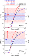 |
Fig. 14 Observed (hatched regions) La and Zr abundances compared to predicted abundances (red and blue dotted curves) as a function of thermal pulse number. For comparison, the evolution of the C/O is also displayed. |
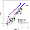 |
Fig. 15 The ([Zr/Fe], [Nb/Fe]) plane. Different kinds of stars are represented by different symbols as labelled in the lower right corner. Abundances for the barium stars are from Karinkuzhi et al. (2018). The error bars on [Zr/Fe] and [Nb/Fe] represent the total uncertainty on the abundances. The red and blue line represent the surface abundance predictions from the models. Each thermal pulse is indicated by a symbol: circles correspond to surface abundances of extrinsic stars, i.e. after the full decay of 93 Zr into Nb, and squares to intrinsic S stars still on the TP-AGB. |
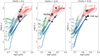 |
Fig. 16 HR diagram of intrinsic (filled triangles) and extrinsic (open squares) S stars along with the STAREVOL evolutionary tracks corresponding to the closest grid metallicity. The red giant branch is represented by the blue dots, the core He-burning phase by the green solid line, whereas the red dashed line corresponds to the AGB tracks. HD 189581 has been moved by − 100 K to avoid overlap with the extrinsic S stars AB Col and V530 Lyr in the left panel. |
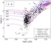 |
Fig. 17 HR diagram of Ba giants and extrinsic S stars superimposed on the STAREVOL evolutionary tracks with [Fe/H] = 0.00 and −0.25. The upper left labels display the typical error bars. |
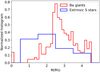 |
Fig. 18 Histogram of the mass distributions for extrinsic S stars from our sample (listed in Table 4) and for the barium giants from Escorza et al. (2017). |
7 Infrared excess of the intrinsic S stars
Infrared excesses observed for AGB stars are associated with the formation of dust; indeed, mass loss and pulsations bring dust far enough from the warm photosphere to allow dust to condensate. Figure 19 compares the SEDs of thethree intrinsic S stars from our sample. There is a clear increase of the infrared excess with decreasing effective temperature for the three stars NQ Pup, V915 Aql and UY Cen (3700, 3400, and 3300 K, respectively). Furthermore, a comparison with Fig. 12 shows that this trend is correlated with the s-process enrichment, since UY Cen is the object with the coolest effective temperature, the largest infrared excess and the largest s-process overabundance. This trend is also well correlated with the C/O (C/O = 0.50, 0.75 and 0.999 for NQ Pup, V915 Aql and UY Cen, respectively; Table 4). These evolutionary indicators point at NQ Pup and V915 Aql as being relatively unevolved intrinsic S stars (at the beginning of the TP-AGB) while UY Cen is among the most evolved intrinsic S stars, consistent with both its location in the HR diagram (well above the predicted onset of TDU) and its spectral classification (S6/8 – Table 1 – or C abundance; Lloyd Evans 2010).
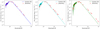 |
Fig. 19 Thespectral energy distributions of NQ Pup, V915 Aql and UY Cen (from left to right), compared with the best-matching spectroscopic MARCS model. |
8 Conclusions
In this paper, we illustrated the specific difficulties faced when trying to derive the atmospheric parameters of S-type stars. Fitting their SED for instance leads to effective temperatures accurate to within 200 K, but does not allow one to fix the other stellar parameters (log g, [Fe/H], C/O, [s/Fe]) without ambiguities. We therefore developed a spectral-fitting method making use of the grid of MARCS model atmospheres for S-type stars. This model grid covers the required range in Teff, surface gravity, metallicity, C/O, and [s/Fe]. The spectral-fitting method finds, among the grid of synthetic spectra, those matching best an observed high-resolution, high S/N spectrum. Combined with Gaia DR2 parallaxes and stellar evolution models, it finally allows one to select the most appropriate model, producing a good agreement at high resolution between synthetic and observed spectra. This provides the necessary basis for deriving reliable surface abundances. The Zr–Nb abundances of extrinsic and intrinsic S stars were especially investigated, and appear to be in good agreement with the predictions of s-process nucleosynthesis in AGB stars. In particular, a segregation is observed between intrinsic (Tc-rich) S stars and extrinsic (barium and S) stars, Tc-rich S stars being, as expected, Nb-poor.
The combination of their atmospheric parameters with their Gaia DR2 parallaxes also provide the location of S stars in the HR diagram. Extrinsic S stars lie either on the upper part of the RGB (for most of them) or on the early-AGB, whereas intrinsic S stars like NQ Pup and UY Cen are located on the TP-AGB (with UY Cen lying well above the onset of TDU episodes). The situation is less clear for the low-mass, Tc-rich S star V915 Aql, pointing at the possible occurrence of TDU episodes in low-mass (M ~ 1 M⊙) stars. For our intrinsic stars, we find a good qualitative correlation between increasing infrared excesses, increasing C/O, increasing s-process overabundance levels, and decreasing effective temperatures. However, another puzzle comes from the tension between the measured and predicted rates at which C/O and s-process abundances increase.
In a forthcoming paper, the Gaia DR2 parallaxes of a larger number of intrinsic S stars will be used in order to constrain the luminosity of the first occurrence of the third dredge-up, as well as the luminosity where the C/O reaches unity (i.e. when S stars turn into SC stars).
Extrinsic S stars appear as the cooler analogs of barium stars in the HR diagram. A comparison of their respective masses reveal, however, that barium stars are on average more massive than extrinsic S stars. This results simply from the fact that, to develop their distinctive ZrO bands, S-type stars should be cooler than ~ 4200 K, and this is possible only close to the RGB tip of low-mass stars. The E-AGB also fulfills this condition, but the shorter time scale associated with that phase does not favour the detection of extrinsic S stars at that stage.
Acknowledgements
This research has been funded by the Belgian Science Policy Office under contract BR/143/A2/STARLAB. S.V.E. thanks Fondation ULB for its support. Based on observations obtained with the HERMES spectrograph, which is supported by the Research Foundation–Flanders (FWO), Belgium, the Research Council of KU Leuven, Belgium, the Fonds National de la Recherche Scientifique (F.R.S.-FNRS), Belgium, the Royal Observatory of Belgium, the Observatoire de Genève, Switzerland and the Thüringer Landessternwarte Tautenburg, Germany. This work has made use of data from the European Space Agency (ESA) mission Gaia (https://www.cosmos.esa.int/gaia), processed by the Gaia Data Processing and Analysis Consortium (DPAC, https://www.cosmos.esa.int/web/gaia/dpac/consortium). Funding for the DPAC has been provided by national institutions, in particular the institutions participating in the Gaia Multilateral Agreement. This research has also made use of the SIMBAD database, operated at CDS, Strasbourg, France. L.S. and S.G. are senior FNRS research associates. DK acknowledges the support from Science and Engineering research Board (SERB), Department of Science and technology (DST), India, through the file number PDF/2017/002338.
Appendix A Line list
Table A.1 lists the lines used for the abundance analysis.
Atomic lines used in this study.
References
- Abia, C., & Wallerstein, G. 1998, MNRAS, 293, 89 [NASA ADS] [CrossRef] [Google Scholar]
- Ake, T. B. 1979, ApJ, 234, 538 [NASA ADS] [CrossRef] [Google Scholar]
- Alvarez, R., & Plez, B. 1998, A&A, 330, 1109 [NASA ADS] [Google Scholar]
- Asplund, M., Grevesse, N., & Sauval, A. J. 2005, ASP Conf. Ser., 336, 25 [Google Scholar]
- Bagnulo, S., Jehin, E., Ledoux, C., et al. 2003, The Messenger, 114, 10 [NASA ADS] [Google Scholar]
- Bailer-Jones, C. A. L., Rybizki, J., Fouesneau, M., Mantelet, G., & Andrae, R. 2018, AJ, 158, 58 [NASA ADS] [CrossRef] [Google Scholar]
- Biémont, E., Grevesse, N., Hannaford, P., & Lowe, R. M. 1981, ApJ, 248, 867 [NASA ADS] [CrossRef] [Google Scholar]
- Biémont, E., Palmeri, P., Quinet, P., et al. 2001, MNRAS, 328, 1085 [NASA ADS] [CrossRef] [Google Scholar]
- Bohlin, R. C., & Gilliland, R. L. 2004, AJ, 127, 3508 [NASA ADS] [CrossRef] [Google Scholar]
- Brown, J. A., Smith, V. V., Lambert, D. L., et al. 1990, AJ, 99, 1930 [NASA ADS] [CrossRef] [Google Scholar]
- Cassisi, S. 2017, Eur. Phys. J. Web Conf., 160, 04002 [Google Scholar]
- Catchpole, R. M. 1982, MNRAS, 199, 1 [NASA ADS] [CrossRef] [Google Scholar]
- Cayrel, R., Depagne, E., Spite, M., et al. 2004, A&A, 416, 1117 [NASA ADS] [CrossRef] [EDP Sciences] [Google Scholar]
- Corliss, C. H., & Bozman, W. R. 1962, NBS Monograph, Experimental Transition Probabilities for Spectral Lines of Seventy Elements, derived from the NBS Tables of spectral-line intensities (US Government Printing Office), 53 [Google Scholar]
- de Boer, E. C. W., & Cottrell, P. L. 2009, ApJ, 692, 522 [NASA ADS] [CrossRef] [Google Scholar]
- Degroote, P., Acke, B., Samadi, R., et al. 2011, A&A, 536, A82 [NASA ADS] [CrossRef] [EDP Sciences] [Google Scholar]
- Den Hartog, E. A., Lawler, J. E., Sneden, C., & Cowan, J. J. 2003, ApJS, 148, 543 [Google Scholar]
- Deroo, P., Reyniers, M., van Winckel, H., Goriely, S., & Siess, L. 2005, A&A, 438, 987 [NASA ADS] [CrossRef] [EDP Sciences] [Google Scholar]
- De Smedt, K., Van Winckel, H., Kamath, D., & Wood, P. R. 2015, A&A, 583, A56 [NASA ADS] [CrossRef] [EDP Sciences] [Google Scholar]
- Drimmel, R., Cabrera-Lavers, A., & López-Corredoira, M. 2003, A&A, 409, 205 [NASA ADS] [CrossRef] [EDP Sciences] [Google Scholar]
- Duquette, D. W., & Lawler, J. E. 1982, Phys. Rev. A, 26, 330 [NASA ADS] [CrossRef] [Google Scholar]
- Escorza, A., Boffin, H. M. J., Jorissen, A., et al. 2017, A&A, 608, A100 [NASA ADS] [CrossRef] [EDP Sciences] [Google Scholar]
- Ferguson, J. W., Alexander, D. R., Allard, F., et al. 2005, ApJ, 623, 585 [NASA ADS] [CrossRef] [Google Scholar]
- Gaia Collaboration (Brown, A. G. A., et al.) 2016, A&A, 595, A2 [NASA ADS] [CrossRef] [EDP Sciences] [Google Scholar]
- Gaia Collaboration (Brown, A. G. A., et al.) 2018, A&A, 616, A1 [NASA ADS] [CrossRef] [EDP Sciences] [Google Scholar]
- García, G., & Campos, J. 1988, J. Quant. Spectr. Rad. Transf., 39, 477 [Google Scholar]
- Gontcharov, G. A. 2012, Astron. Lett., 38, 87 [NASA ADS] [CrossRef] [Google Scholar]
- Goriely, S., & Mowlavi, N. 2000, A&A, 362, 599 [NASA ADS] [Google Scholar]
- Goriely, S., & Siess, L. 2018, A&A, 609, A29 [NASA ADS] [CrossRef] [EDP Sciences] [Google Scholar]
- Grevesse, N., Asplund, M., & Sauval, A. J. 2007, Space Sci. Rev., 130, 105 [Google Scholar]
- Hannaford, P., & Lowe, R. M. 1985, J. Phys. B At. Mol. Phys., 18, 2365 [NASA ADS] [CrossRef] [Google Scholar]
- Hillen, M., Van Winckel, H., Menu, J., et al. 2017, A&A, 599, A41 [NASA ADS] [CrossRef] [EDP Sciences] [Google Scholar]
- Høg, E., Fabricius, C., Makarov, V. V., et al. 2000, A&A, 355, L27 [Google Scholar]
- Iben, Jr. I., & Renzini, A. 1983, ARA&A, 21, 271 [NASA ADS] [CrossRef] [Google Scholar]
- Iglesias, C. A., & Rogers, F. J. 1996, ApJ, 464, 943 [NASA ADS] [CrossRef] [Google Scholar]
- Jorissen, A. 2004, in AGB Stars, eds. H. Habing & H. Olofsson (New York: Springer Verlag), 461 [Google Scholar]
- Jorissen, A., & Mayor, M. 1988, A&A, 198, 187 [NASA ADS] [Google Scholar]
- Jorissen, A., Frayer, D. T., Johnson, H. R., Mayor, M., & Smith, V. V. 1993, A&A, 271, 463 [NASA ADS] [Google Scholar]
- Käppeler, F., Gallino, R., Bisterzo, S., & Aoki, W. 2011, Rev. Mod. Phys., 83, 157 [NASA ADS] [CrossRef] [EDP Sciences] [Google Scholar]
- Karakas, A. I., & Lugaro, M. 2016, ApJ, 825, 26 [NASA ADS] [CrossRef] [Google Scholar]
- Karinkuzhi, D., Van Eck, S., Jorissen, A., et al. 2018, A&A, 618, A32 [NASA ADS] [CrossRef] [EDP Sciences] [Google Scholar]
- Kurucz, R. L. 2007, Robert L. Kurucz on-line database of observed and predicted atomic transitions [Google Scholar]
- Lawler, J. E., Bonvallet, G., & Sneden, C. 2001, AJ, 556, 452 [Google Scholar]
- Lawler, J. E., Den Hartog, E. A., Sneden, C., & Cowan, J. J. 2006, ApJS, 162, 227 [NASA ADS] [CrossRef] [Google Scholar]
- Little, S. J., Little-Marenin, I. R., & Bauer, W. H. 1987, AJ, 94, 981 [NASA ADS] [CrossRef] [Google Scholar]
- Little-Marenin, I. R., & Little, S. J. 1979, AJ, 84, 1374 [NASA ADS] [CrossRef] [Google Scholar]
- Lloyd Evans T. 2010, JApA, 31, 177 [NASA ADS] [CrossRef] [Google Scholar]
- Maíz Apellániz J. 2007, in The Future of Photometric, Spectrophotometric and Polarimetric Standardization, ed. Sterken, C. ASP Conf. Ser., 364, 227 [Google Scholar]
- Marigo, P. 2002, A&A, 387, 507 [NASA ADS] [CrossRef] [EDP Sciences] [Google Scholar]
- Martin, G., Fuhr, J., & Wiese, W. 1988, J. Phys. Chem. Ref. Data Suppl., 17, 872 [Google Scholar]
- Meggers, W. F., Corliss, C. H., & Scribner, B. F. 1975, Tables of spectral-line intensities. Part I, II - Arranged by Elements (US Government Printing Office) [Google Scholar]
- Merle, T., Jorissen, A., Van Eck, S., Masseron, T., & Van Winckel H. 2016, A&A, 586, A151 [NASA ADS] [CrossRef] [EDP Sciences] [Google Scholar]
- Merrill, P. W. 1922, ApJ, 56, 457 [NASA ADS] [CrossRef] [Google Scholar]
- Merrill, P. W. 1952, ApJ, 116, 21 [NASA ADS] [CrossRef] [Google Scholar]
- Miles, B. M., & Wiese, W. L. 1969, At. Data, 1, 1 [Google Scholar]
- Nave, G., Johansson, S., Learner, R. C. M., Thorne, A. P., & Brault, J. W. 1994, ApJS, 94, 221 [NASA ADS] [CrossRef] [Google Scholar]
- Neyskens, P., Van Eck, S., Jorissen, A., et al. 2015, Nature, 517, 174 [NASA ADS] [CrossRef] [PubMed] [Google Scholar]
- Nilsson, A. E., Johansson, S., & Kurucz, R. L. 1991, Phys. Scr, 44, 226 [Google Scholar]
- O’Brian, T. R., Wickliffe, M. E., Lawler, J. E., Whaling, W., & Brault, J. W. 1991, J. Opt. Soc. Am. B Opt. Phys., 8, 1185 [NASA ADS] [CrossRef] [Google Scholar]
- Otto, E., Green, P. J., & Gray, R. O. 2011, ApJS, 196, 5 [NASA ADS] [CrossRef] [Google Scholar]
- Palmeri, P., Quinet, P., Wyart, J., & Biémont, E. 2000, Phys. Scr., 61, 323 [NASA ADS] [CrossRef] [Google Scholar]
- Penkin, N. P., & Komarovskii, V. A. 1976, J. Quant. Spectr. Rad. Transf., 16, 217 [Google Scholar]
- Piccirillo, J. 1980, MNRAS, 190, 441 [NASA ADS] [Google Scholar]
- Plez, B. 2012, Astrophysics Source Code Library [record ascl:1205.004] [Google Scholar]
- Raassen, A. J. J., & Uylings, P. H. M. 1998, A&A, 340, 300 [NASA ADS] [Google Scholar]
- Raskin, G., van Winckel, H., Hensberge, H., et al. 2011, A&A, 526, A69 [NASA ADS] [CrossRef] [EDP Sciences] [Google Scholar]
- Scalo, J. M., & Miller, G. E. 1981, ApJ, 246, 251 [NASA ADS] [CrossRef] [Google Scholar]
- Schröder, K.-P., & Cuntz, M. 2007, A&A, 465, 593 [NASA ADS] [CrossRef] [EDP Sciences] [Google Scholar]
- Siess, L., & Arnould, M. 2008, A&A, 489, 395 [NASA ADS] [CrossRef] [EDP Sciences] [Google Scholar]
- Siess, L., Dufour, E., & Forestini, M. 2000, A&A, 358, 593 [Google Scholar]
- Skrutskie, M. F., Cutri, R. M., Stiening, R., et al. 2006, AJ, 131, 1163 [NASA ADS] [CrossRef] [Google Scholar]
- Smith, V. V., & Lambert, D. L. 1988, ApJ, 333, 219 [NASA ADS] [CrossRef] [Google Scholar]
- Smith, V. V., & Lambert, D. L. 1990, ApJS, 72, 387 [NASA ADS] [CrossRef] [Google Scholar]
- Stephenson, C. B. 1984, Publications of the Warner & Swasey Observatory, 3, 1 [Google Scholar]
- Van Eck, S., & Jorissen, A. 1999, A&A, 345, 127 [NASA ADS] [Google Scholar]
- Van Eck, S., & Jorissen, A. 2000, A&A, 360, 196 [NASA ADS] [Google Scholar]
- Van Eck, S., Jorissen, A., Udry, S., Mayor, M., & Pernier, B. 1998, A&A, 329, 971 [NASA ADS] [Google Scholar]
- Van Eck, S., Jorissen, A., Udry, S., et al. 2000, A&AS, 145, 51 [NASA ADS] [CrossRef] [EDP Sciences] [Google Scholar]
- Van Eck, S., Neyskens, P., Jorissen, A., et al. 2017, A&A, 601, A10 [Google Scholar]
- Vassiliadis, E., & Wood, P. R. 1993, ApJ, 413, 641 [NASA ADS] [CrossRef] [Google Scholar]
- Wang, X.-H., & Chen, P.-S. 2002, A&A, 387, 129 [NASA ADS] [CrossRef] [EDP Sciences] [Google Scholar]
- Wenger, M., Ochsenbein, F., Egret, D., et al. 2000, A&AS, 143, 9 [NASA ADS] [CrossRef] [EDP Sciences] [Google Scholar]
HERMES is an acronym for High Efficiency and Resolution Mercator Echelle Spectrograph.
To be consistent in this comparison with SVE17, we computed the reddening EB−V using the 3D Galactic Extinction Model of Drimmel et al. (2003) and used that value as the upper limit on EB−V.
The spectroscopic method applicable for hotter stars, using excitation and ionisation equilibrium to constrain Teff and log g, cannot be used here. Indeed, given the heavily blended and depressed spectra of S stars and the current accuracy of transition probabilities and wavelengths in molecular (mainly TiO, ZrO, LaO, VO and CH) line lists, a χ2 minimization between synthetic and observed spectra has to be performed instead.
All Tables
Stellar parameters for a set of Henize stars obtained from SVE17, compared with results from S4U.
Elemental abundances for NQ Pup, UY Cen, and V915 Aql, along with the standard deviation due to line-to-line scatter.
Sensitivity of the elemental abundances of NQ Pup upon variations of the atmospheric parameters.
All Figures
|
Fig. 1 Error on the parallax σϖ as a function of the parallax ϖ for the 124 S stars resulting from the intersection of the General Catalog of Galactic S stars (Stephenson 1984) and Gaia DR1 (Gaia Collaboration 2016), observable with the HERMES spectrograph (δ > −30°). The blue and green lines delineate the quality conditions defined as σϖ = 0.3 ϖ and σϖ = 0.5 ϖ, respectively. |
| In the text | |
|
Fig. 2 The spectral region around the three (4238.19, 4262.27 and 4297.06 Å) ultra-violet Tc I lines in Tc-poor S stars. The observed spectra have been normalized using unity-based normalization. |
| In the text | |
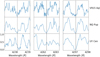 |
Fig. 3 Same as Fig. 2 for Tc-rich S stars. |
| In the text | |
|
Fig. 4 Top left panel: SED fitting of V915 Aql using S4U where the red line represents the MARCS model best matching the photometric observations collected from SIMBAD. Top right panel: probability distribution plot of log g vs Teff for V915 Aql obtained using S4U. Bottom left panel: same as top right panel but for [C/Fe] vs Teff and bottom rightpanel for [s/Fe] vs Teff. The red plus sign in top right, bottom left and right panels indicates the best model selected by S4U. |
| In the text | |
|
Fig. 5 Iterating scheme to constrain logg. |
| In the text | |
|
Fig. 6 Carbon abundance derived from a comparison between the observed spectrum of the extrinsic S star HD 189581 in the CH G-band (black line) and the synthetic spectrum for different C/O values. The best agreement is obtained for C/O = 0.5. The grey line presents the synthesis without the CH linelist. |
| In the text | |
|
Fig. 7 Bottom panel: comparison between the synthetic and observed spectra for V530 Lyr in the 8076–8088 Å range containing CN lines. Top three panels: ±1 Å zoom around the CN lines at 8035, 8057.3, and 8082.9 Å (from left to right panels). The green dashed lines mark the CN lines used by Merle et al. (2016) in barium stars. The grey line presents the synthesis without the CN line list. The value [N/Fe] = 0.9 has been adopted. |
| In the text | |
|
Fig. 8 Illustration of the quality of the match between observed and synthetic spectra obtained for the extrinsic S star V530 Lyr around the Zr line at 7849.37 Å. The upper panel presents a ± 3Å zoom. |
| In the text | |
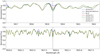 |
Fig. 9 Same as Fig. 8 for the intrinsic S star V915 Aql around the Zr line at 7819.37 Å. |
| In the text | |
|
Fig. 10 Comparison between the observed spectrum of V915 Aql (black line) and synthetic spectra corresponding to model A (top panel, blue line) and to model H (bottom panel, red line), in the region surrounding the Zr I λ7819 Å line. |
| In the text | |
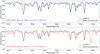 |
Fig. 11 Same as Fig. 10 for NQ Pup in one of the TiO band. |
| In the text | |
|
Fig. 12 Abundances of the three intrinsic S stars, with C and N (top panel), light s-process elements (middle panel) and heavy s-process elements (bottom panel). The error bars on the elemental abundances represent the total uncertainty calculated by quadratically summing the Δ H−A values from the last columns of Tables 7–9 with the standard deviation due to line-to-line scatter, plusan extra 0.1 dex as uncertainty due to continuum placement. |
| In the text | |
|
Fig. 13 Left panels: location of the three intrinsic S stars in the HR diagram, compared with STAREVOL tracks of the corresponding metallicity. Right panels: predicted abundance distribution of the three intrinsic S stars. Top panels: NQ Pup, centralpanels: V915 Aql, and bottom panels: UY Cen. |
| In the text | |
|
Fig. 14 Observed (hatched regions) La and Zr abundances compared to predicted abundances (red and blue dotted curves) as a function of thermal pulse number. For comparison, the evolution of the C/O is also displayed. |
| In the text | |
|
Fig. 15 The ([Zr/Fe], [Nb/Fe]) plane. Different kinds of stars are represented by different symbols as labelled in the lower right corner. Abundances for the barium stars are from Karinkuzhi et al. (2018). The error bars on [Zr/Fe] and [Nb/Fe] represent the total uncertainty on the abundances. The red and blue line represent the surface abundance predictions from the models. Each thermal pulse is indicated by a symbol: circles correspond to surface abundances of extrinsic stars, i.e. after the full decay of 93 Zr into Nb, and squares to intrinsic S stars still on the TP-AGB. |
| In the text | |
|
Fig. 16 HR diagram of intrinsic (filled triangles) and extrinsic (open squares) S stars along with the STAREVOL evolutionary tracks corresponding to the closest grid metallicity. The red giant branch is represented by the blue dots, the core He-burning phase by the green solid line, whereas the red dashed line corresponds to the AGB tracks. HD 189581 has been moved by − 100 K to avoid overlap with the extrinsic S stars AB Col and V530 Lyr in the left panel. |
| In the text | |
|
Fig. 17 HR diagram of Ba giants and extrinsic S stars superimposed on the STAREVOL evolutionary tracks with [Fe/H] = 0.00 and −0.25. The upper left labels display the typical error bars. |
| In the text | |
|
Fig. 18 Histogram of the mass distributions for extrinsic S stars from our sample (listed in Table 4) and for the barium giants from Escorza et al. (2017). |
| In the text | |
|
Fig. 19 Thespectral energy distributions of NQ Pup, V915 Aql and UY Cen (from left to right), compared with the best-matching spectroscopic MARCS model. |
| In the text | |
Current usage metrics show cumulative count of Article Views (full-text article views including HTML views, PDF and ePub downloads, according to the available data) and Abstracts Views on Vision4Press platform.
Data correspond to usage on the plateform after 2015. The current usage metrics is available 48-96 hours after online publication and is updated daily on week days.
Initial download of the metrics may take a while.