| Issue |
A&A
Volume 619, November 2018
|
|
|---|---|---|
| Article Number | A133 | |
| Number of page(s) | 8 | |
| Section | Celestial mechanics and astrometry | |
| DOI | https://doi.org/10.1051/0004-6361/201833930 | |
| Published online | 15 November 2018 | |
Strong tidal energy dissipation in Saturn at Titan’s frequency as an explanation for Iapetus orbit
1 IMCCE, Observatoire de Paris, PSL Research University, CNRS, UPMC Univ. Paris 06, Univ. Lille, France
e-mail: This email address is being protected from spambots. You need JavaScript enabled to view it.
2 Jet Propulsion Laboratory, California Institute of Technology, Pasadena, USA
3 Namur Institute for Complex Systems (naXys), University of Namur, Belgium
Received:
23
July
2018
Accepted:
6
September
2018
Abstract
Context. Natural satellite systems present a large variety of orbital configurations in the solar system. While some are clearly the result of known processes, others still have largely unexplained eccentricity and inclination values. Iapetus, the furthest of Saturn’s main satellites, has a still unexplained 3% orbital eccentricity and its orbital plane is tilted with respect to its local Laplace plane (8° of free inclination). On the other hand, astrometric measurements of saturnian moons have revealed high tidal migration rates, corresponding to a quality factor Q of Saturn of around 1600 for the mid-sized icy moons.
Aims. We show how a past crossing of the 5:1 mean motion resonance between Titan and Iapetus may be a plausible scenario to explain Iapetus’ orbit.
Methods. We have carried out numerical simulations of the resonance crossing using an N-body code as well as using averaged equations of motion. A large span of migration rates were explored for Titan and Iapetus was started on its local Laplace plane (15° with respect to the equatorial plane) with a circular orbit.
Results. The resonance crossing can trigger a chaotic evolution of the eccentricity and the inclination of Iapetus. The outcome of the resonance is highly dependent on the migration rate (or equivalently on Q). For a quality factor Q of over around 2000, the chaotic evolution of Iapetus in the resonance leads in most cases to its ejection, while simulations with a quality factor between 100 and 2000 show a departure from the resonance with post-resonant eccentricities spanning from 0 up to 15%, and free inclinations capable of reaching 11°. Usually high inclinations come with high eccentricities but some simulations (less than 1%) show elements compatible with Iapetus’ current orbit
Conclusions. In the context of high tidal energy dissipation in Saturn, a quality factor between 100 and 2000 at the frequency of Titan would bring Titan and Iapetus into a 5:1 resonance, which would perturb Iapetus’ eccentricity and inclination to values observed today. Such rapid tidal migration would have avoided Iapetus’ ejection around 40–800 million years ago.
Key words: chaos / methods: numerical / celestial mechanics / planets and satellites: dynamical evolution and stability
© ESO 2018
1. Introduction
Mean motion resonances in planetary systems have been the subject of many studies throughout the last century, up to the present day. It has been established that mean motion ratios that are close to rational values are very unlikely to be the effect of randomness (Roy & Ovenden 1954), being instead the result of a series of mechanisms involving satellite migration and subsequent capture into stable mean motion resonant configurations (Goldreich 1965a). The system formed by Saturn and its eight major satellites (Mimas, Enceladus, Tethys, Dione, Rhea, Titan, Hyperion, and Iapetus) is a unique system in which one can find several of its moons evolving in a resonance. We have Mimas and Tethys, locked in a 4:2 mean motion resonance, responsible for their growth in inclination; Enceladus and Dione whose periods are commensurable, yielding a 2:1 resonance that explains the eccentricity of Enceladus (and is a direct cause of the heating of Enceladus); and finally Titan and the small moon Hyperion, which keep their orbital periods in a 4:3 resonance, Titan being known to drive Hyperion’s orbit thanks to this resonance (Colombo et al. 1974).
Today it is believed that tides from satellites acting on the planet are responsible for satellite resonances, the latter preserving the commensurability as the satellites continue evolving outwards. The general theory would relate the growth of the semi-major axis of the satellite to the dissipation acting inside the planet. Such a theory is applicable to solid bodies like our Earth but it is not straightforward to apply it to gaseous bodies such as giant planets or stars. However, scientists usually keep the dissipative approach and relate satellite migration to the quality factor Q, which measures the energy dissipation inside the planet.
However, the Saturn system has recently been targeted by astrometry. First, the spacecraft Cassini, in orbit around Saturn between 2004 and 2017, was a key instrument for the measurements of the positions of Saturn’s satellites throughout its mission (Cooper et al. 2018). Many Earth-based observations of this system were also made in the last hundred years. Making use of all these measurements, Lainey et al. (2017) fitted an average quality factor Q of around 1600 at the orbital frequency of the icy moons Enceladus, Tethys, and Dione, which is more than an order a magnitude smaller than the theoretical value attributed to Saturn’s dissipation by Goldreich & Soter (1966). In addition, the quality factor at Rhea’s frequency was found to be around 300, not only confirming a fast tidal recession for this moon but also suggesting that the quality factor could be a frequency-dependent parameter. These high dissipation values may be explained by viscous friction in a solid core in Saturn (Remus et al. 1991), resulting in a fast expansion of the orbits.
Assuming high Q at Mimas’s frequency (Goldreich & Soter 1966), some authors suggested that Q could still be around 2000 at Titan’s frequency (Greenberg 1973; Colombo et al. 1974). A more recent theory (Fuller et al. 2016) gave a explanation for the low and frequency-dependent values of Q found in Lainey et al. (2017). Applied to Titan, Q would be around 25 (Fuller et al. 2016).
These fast tidal recessions allow for the possibility of past resonance crossings. If Titan had been migrating very rapidly in its history (Q ⪅ 14 000), it would have crossed a 5:1 mean motion resonance with Iapetus. Therefore, in this study, we explore several values of Q at Titan’s frequency with a particular emphasis on low values (2–5000). We simulate a 5:1 mean motion resonance crossing with Iapetus over a few million to hundreds of millions of years. Iapetus is today on an eccentric orbit (eI ≈ 0.03) and its orbital plane has an 7.9° tilt with respect to its local Laplace plane (Fig. 1). If created from its circumplanetary disk, the tilt should have been null (Nesvorný et al. 2014). Some authors have proposed some plausible scenarios to explain these values. Ward (1981) invoked a fast dispersal of the circumplanetary disk from which satellites were formed. Iapetus would have evolved to the orbit we see today if the disk was dispersed in around 102 or 103 years, which is a fast timescale for this process to happen. Also, in the context of the early solar system instability (Tsiganis et al. 2005), Nesvorný et al. (2014) argue that Iapetus could have been excited by close encounters between an ice giant and the system of Saturn. However, we looked for an alternative scenario where the 5:1 resonance would be responsible for its orbital behaviour.
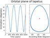 |
Fig. 1. Motion of Iapetus plane over 10 000 years. Both the inclination and the longitude of the ascending node oscillate around the fixed values of the Laplace plane with a period of around 3200 years. Here, and for the rest of this work, the reference plane is the equator of Saturn. The figure comes from a simulation done with all the major satellites of Saturn (Mimas, Enceladus, Tethys, Dione, Rhea, Titan, Hyperion, Iapetus), the Sun, and the effect of the flattening of Saturn. The angular elements of the Laplace plane are approximately 15° for the inclination and 225° for the ascending node. The initial conditions are those of the J2000 epoch taken from JPL ephemeris, Horizon (SAT 389.14). |
We first introduce the general theory of a satellite orbiting on or close to its Laplace plane. Then, after explaining the different methods used for this research, we describe the results of several simulations made numerically with an N-body code, or using averaged equations of motion. Finally, the article ends with some discussion on the method and the conclusions.
2. The Laplace plane
Iapetus’ orbital plane is actually tilted with respect to several important planes. First, due to the relatively large distance of the satellite from the planet, the effect coming from the Sun is more pronounced than for the other satellites. Iapetus does not orbit in the planet’s equator. Its orbital plane secularly oscillates around a specific plane called the Laplace plane. The latter is a fixed plane with an inclination of about 15° with respect to the equator. Orbiting close to it, a satellite would also have its ascending node oscillating around a fixed value, corresponding to the Sun’s ascending node. It is defined as an equilibrium between the pull of the Sun and the flattening effect of the planet and the inner satellites. The orbit of Iapetus is tilted with respect to this plane with an angle of about 7.9°. On top of this, its eccentricity is around 0.03. We consider that both values still need an explanation. We assume that a satellite would be created on its Laplace plane after being formed from a circumplanetary disk (Nesvorný et al. 2014).
To set the general equations for the Laplace plane, we start with the perturbing acceleration of a body j acting upon a body i,
 (1)
(1)
where ri denotes the position vector of the ith satellite, with mass mi, and the unbold ri its magnitude. So rij stands for the separation between satellites i and j, |ri − rj|. The mass of Saturn is denoted by mS and G stands for the gravitational constant. The right-hand side of this equation can be rewritten ∇iRj, where Rj stands for the disturbing function of the body j acting on i,
 (2)
(2)
In our case, the reference frame is centred on Saturn and the Sun acts as an external satellite around the planet. The disturbing function for the Sun can therefore be expanded in terms of Legendre polynomials (Murray & Dermott 2000; Brouwer & Clemence 1961),
 (3)
(3)
Here the subscript i stands for any satellite and ψ denotes the angle between the position vectors of the Sun and the satellite, verifying the relation ri.r⊙ = rir⊙ cos (ψ). After some quick manipulations1 (Brouwer & Clemence 1961), terms in series Eq. (3) appear proportional to αl, α being the semi-major axis ratio, which is small in the case of planetary satellites2. Therefore, we limit ourselves to the first term in the series, l = 2,
![Mathematical equation: $$ \begin{aligned} R_{\odot }=n_{\odot }^{2}a_{i}^{2}\left[\left(\frac{r_{i}}{a_{i}}\right)^{2}\left(\frac{a_{\odot }}{r_{\odot }}\right)^{3}\left(-\frac{1}{2}+\frac{3}{2}\cos ^{2}(\psi )\right)+O(\alpha ^{2})\right] .\end{aligned} $$](/articles/aa/full_html/2018/11/aa33930-18/aa33930-18-eq4.gif) (4)
(4)
Using several expansions developed in Murray & Dermott (2000), and after averaging over the mean longitudes of the satellite and the Sun, we obtain eight different arguments with  Then, the satellites also undergo the effect of the flattening of Saturn; the disturbing function related to this effect can be written as
![Mathematical equation: $$ \begin{aligned} R_{\rm J_{2}}=\frac{G\left(m_{\rm S}+m_{i}\right)Rp^{2}J^\prime _{2}\left[1+3\cos (2i)\right]}{8a^{3}\left(1-e^{2}\right)^{3/2}} ,\end{aligned} $$](/articles/aa/full_html/2018/11/aa33930-18/aa33930-18-eq6.gif) (5)
(5)
with Rp the equatorial radius of Saturn. Here, it is important to underline that  not only corresponds to the zonal harmonic of Saturn, but to a general flattening seen by a satellite, made of the proper flattening of the planet and by the secular effect of the interior satellites. We define (Tremaine et al. 2009)
 (6)
(6)
As a consequence, Titan and Iapetus do not see the same “flattening”. Titan undergoes the flattening of the planet and the inner icy satellites (Mimas to Rhea), which do not participate much, while it plays a major role in the  for Iapetus. We form the disturbing function formed by those two effects,
 (7)
(7)
and plug it into the Lagrange Planetary Equations
 (8)
(8)
 (9)
(9)
A satellite orbiting on its local Laplace plane will see its orbital plane fixed in time, meaning that the rates of the ascending node and the inclination are null. The local Laplace plane orbital elements therefore verify
 (10)
(10)
which possess several solutions (see Fig. 2). The solution we are interested in imposes
 (11)
(11)
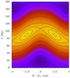 |
Fig. 2. Level curve of the Hamiltonian from Eq. (7). Orbital plane elements will follow the solid lines. One can distinguish four different kinds of equilibrium: one for retrograde orbits, two for polar orbits, and the one we are interested in, for relatively low inclination. The latter gives us Ω = Ω⊙ and both ascending nodes of Iapetus and Titan oscillate around it. Equation (12) and Table 2 give an inclination of the local Laplace plane of Titan around 0.62°. |
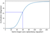 |
Fig. 3. Tilt of Iapetus’ local Laplace plane to Saturn’s equator as a function of Iapetus’ semi-major axis. Here |

The inclination and ascending node of the Laplace plane are those verifying formula (11). We see in Fig. 1 that the ascending node oscillates around a fixed value. This value is actually that of the Sun, Ω⊙, which was around 225° for this specific simulation. In the rest of this study we have set Ω⊙ = 0. The equilibrium inclination, iLP, can be found by rewriting the first equation of formula (11),
 (12)
(12)
where
 (13)
(13)
and
 (14)
(14)
so that for  and
and 
 (15)
(15)
The function F(e⊙, ei) contains the dependency on both eccentricities,
 (16)
(16)
Eccentricities do not play a major role in the equilibrium if they stay small. However, if we consider the action of other planets, the eccentricity of Saturn (or the Sun in our model) will change, changing slightly the position of the Laplace plane.
We have derived here the equation for the inclination of the Laplace plane. Equation (12) can also be found in Tremaine et al. (2009) and in Nesvorný et al. (2014). For Titan and Iapetus, it is a forced plane around which their orbit will evolve. In our case, Iapetus is assumed to have formed on its Laplace plane, therefore we chose it as the initial orbital plane of the satellite in our simulations.
3. Tides
The start of this research was motivated by the low values of the quality factor Q found at the frequency of the inner icy satellites in Lainey et al. (2012, 2017). Furthermore, Fuller et al. (2016) published a theory in which those dissipative values matched the ones found by astrometry. Fuller’s model also predicts a quality factor of around 25 for Titan if we consider a tidal timescale of around two billion years (second equation in Fuller’s paper), as was chosen for other satellites in the paper. Fuller’s model predicts that resonance locking can be reached due to the internal structural evolution of the planet. Moons are then “surfing” on dissipation peaks and migrate outwards at rates comparable to the ones found by astrometry. We assume relatively high migration rates for Titan by choosing a quality factor spanning from 2 to around 5000, but also higher values were tested to be able to make a full comparison. The following tidal acceleration was implemented in our software (Efroimsky & Lainey 2007):
 (17)
(17)
with
 (18)
(18)
and
 (19)
(19)
Here k2 denotes the second order Love number, Rp is the equatorial radius of Saturn, G the gravitational constant, mS, Saturn’s mass, mi the satellite’s mass, ri its positional vector and its norm ri, v i its velocity vector, and ΩS the rotational spin axis of the planet. For the latter, Saturn’s rotational period is taken to be 0.44401 days.
This tidal equation will introduce a secular increase of Titan’s semi-major axis, following
 (20)
(20)
and also of its eccentricity, but the change is negligible. This tidal model will not produce the same migration of satellite on a long timescale as the model proposed in Fuller et al. (2016), but here we are looking for a classical tidal model producing a constant time rate of the semi-major axis through the resonance. We underline here that tidal theories were first produced for solid bodies. In these theories, the satellite creates a bulge on the planet through differential acceleration, but this bulge would not align instantaneously with the satellite because of the viscoelasticity of the primary (Kaula 1964; Mignard 1991). The quality factor Q introduced in Eqs. (18) and (20) would measure the energy dissipated inside the planet. The consequence of this lag is the triggering of angular momentum exchange between the planet spin and the orbit of the satellite. Whether this angular momentum exchange happens in the core or in the envelope of the planet is still under investigation. However, it is understood that the core can strongly contribute to the tidal acceleration of satellites due to internal dissipation and the existence of a solid inner core in Saturn has been recently reconsidered (Remus et al. 1991; Guenel et al. 2014). The convective envelope would be subjected to matter redistribution and modification of the velocity field in the presence of a tidal potential (Remus et al. 1991). This could also trigger some viscous friction and exchange of angular momentum between the planet and the satellite (Zahn 1966). Bodely tides formalism can also apply to fluid envelops (Efroimsky 2012). Instead of using the notion of energy dissipation, one can use its counterpart in terms of semi-major axis growth with Eq. (20). Unless one chooses a very low value of Q, the semi-major axis of Titan will not change drastically during the resonance crossing. Therefore we can plug constant values into the right-hand side of Eq. (20). Rewritten in units of Titan’s initial semi-major axis and million years, the semi-major axis rate would be approximately
 (21)
(21)
For instance, for Q = 100, Titan increases 0.01% of its initial semi-major axis in a million years.
4. Methods
4.1. Summary of the physical model
All the above equations are set with the origin of the reference frame centred in Saturn, from which the x and y axes lie in the equatorial plane of the planet and the z axis points towards the north pole. The study involves Titan and Iapetus, but in order to catch the correct dynamics, we have shown that the gravitational attraction of the Sun has to be added. It was placed on an orbit with a 26.73° inclination, which corresponds to Saturn’s obliquity. The presence of Hyperion is also important since it lies in a 4:3 mean motion resonance with Titan. We have kept track of such a dynamical configuration. The contributions coming from other satellites were merged with the flattening effect of the planet by defining an upgraded J2 effect (Eq. (6)). The gravity of the other planets has been neglected, but nevertheless, the action of Jupiter adds a small secular oscillation to the Laplace plane equilibrium. It will be discussed at the end of the paper. Finally, Titan would tidally migrate during the simulation, with a rate depending on the quality factor of Saturn (Eq. (20)). Finally, we neglect Iapetus’ migration.
4.2. Direct-N-body integration and averaged equations
Two different methods have been used. The first and more direct is an integration of the positions and velocities of the bodies using an implicit Gauss–Radau scheme like in Everhart (1974), Everhart (1985), and Rein & Spiegel (2015). This method, although precise, is time-consuming and needs a good amount of hardware power. Simulations involving a parameter Q below 1500 were done using this approach, but for higher values of the quality factor, averaged equations of motion were used. In this approach, we used non-singular coordinates to avoid any singularity problem, as Titan orbits close to the equator and Iapetus’ orbit was chosen as circular at the beginning of the integration. Effects coming from the flattening of Saturn were implemented by using partial derivatives of Eq. (5) with respect to those coordinates and then plugged into the Lagrange Planetary Equations. Tides were added by using Eq. (20) and the averaged effect of the Sun is well represented by the eight terms in Table 1. In order to get a good approximation for the mutual influence of the satellite, we chose to use the method developed in Murray & Dermott (2000). Titan acts like a internal perturber for Iapetus and Iapetus like an external one for Titan, therefore the disturbing function for those two satellites can be written as
 (22)
(22)
 (23)
(23)
Terms coming from the disturbing function of the Sun acting on both satellites.
Flattening parameters seen by both satellites.
Using this notation, Iapetus’ dynamics, for instance, will be given by first taking the partial derivatives of RTitan with respect to Iapetus coordinates, and then plugged into the Lagrange Planetary Equations. For both Eqs. (22) and (23), RD is the direct part of the disturbing function
 (24)
(24)
Here, RI and RE are the indirect part of the disturbing function for the internal and external perturber. Each of those terms has an explicit development shown in Murray & Dermott (2000) and we have made an intensive use of them. Terms appearing in the development have the general form
 (25)
(25)
where the d’Alembert rule imposes that the sum of the integer coefficients ji vanishes and that by symmetry, j5 + j6 is always an even number. In our case, we are studying dynamics that involve a close or exact 5:1 commensurability between the mean motion of the satellites. Therefore, we limit ourselves to two types of arguments: those with no mean longitudes appearing, which we call the secular terms, and those that have 5λI − λT in their expression. We call those resonant terms. Terms other than those mentioned are averaged out. For resonant terms, we have the relation
 (26)
(26)
imposed by the d’Alembert rule. The function S depends on the eccentricities, inclinations, and the semi-major axis ratio, which relates to the cosine argument in the following way:
 (27)
(27)
The expansion in Murray & Dermott (2000) assumes that eccentricities and inclinations are small, and a fourth order expansion would mean
 (28)
(28)
anywhere in the expansion. However, in our case we have to account for the fact that Iapetus’ orbital plane is far from being equatorial. On average the inclination will be 15°, the tilt of the Laplace plane. Therefore sI is not small and the consequence is that higher powers of it have to be added to ensure a correct expansion. On the other hand, Titan’s local Laplace plane is close to the equator and sT < 0.01 during its evolution. Therefore no power higher than 2 for sT will be considered. For eccentricities, we had to go up to fourth powers because it is a resonance of order 4 Table 3.
This redefines the idea we have of the order of the expansion. The following constraints where used to truncate our expansion:
 (29)
(29)
with
 (30)
(30)
and j5 is left unconstrained, but we have truncated the expansion in s8 when the numerical evaluation of the disturbing term stopped showing a significant change. The resulting expansion for the direct part has 31 secular and 61 resonant terms. Here is an example of a term
 (31)
(31)
where Φ are functions of the semi-major axis ratio only involving the Laplace coefficients and their derivatives.
5. Simulation results
In this section, we show several results coming from numerical simulations. The eccentricity and the inclination can both be affected by the mean motion resonance crossing in general. Both elements can behave chaotically during the crossing and their resulting values are unpredictable. On the other hand, simulations have shown “smooth” resonance captures, in which either the eccentricity or the inclination evolve smoothly (Fig. 4). The great majority of them came from the N-body code and an analysis of all simulations shows that this behaviour happens more often for high values of Q (Table 4). However, because only one element evolves we have discarded these evolutions as a possible scenario.
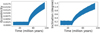 |
Fig. 4. Smooth evolutions of the eccentricity and the inclination coming from two different simulations. On the left, the eccentricity of Iapetus growths smoothly after both satellites enter the resonance, while the tilt stays constant. The right figure depicts the evolution of the inclination with respect to the Laplace plane. For this simulation, the eccentricity does not change. |
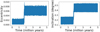 |
Fig. 5. Example of a resonance crossing with Q = 50 using the N-body code. The obvious effect of the resonance is here a “kick” in both eccentricity and free inclination. |
Numbers of smooth evolutions as a function of Q using the N-body code.
We have concentrated our analysis on the chaotic evolutions and one can distinguish two different types:
-
Fast crossings, for Q under 100. Usually, Titan rushes through the resonance and this prevents any capture. Still, the effect on the eccentricity of Iapetus can result in a kick of a few percent, reaching sometimes 0.05. On the other hand, the inclination is not really affected at this point. A few degrees can be obtained in the best cases.
-
For values of Q over 100, the majority of simulations show a capture and a chaotic evolution of Iapetus’ orbit. Then, several scenarios can take place. Either the capture is maintained and its eccentricity grows until Iapetus is ejected from the system; or Iapetus is released from the resonance and continues on a regular orbit with an excited eccentricity and inclination as shown in Fig. 6 .
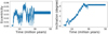
Fig. 6. Example figures of outputs obtained from our simulations. In this example we clearly distinguish a regular evolution before the resonance, a chaotic resonance crossing, and finally regular dynamics after the resonance. In this specific example, the eccentricity increase is around 0.035 and the tilt has grown to around 4.5. These two figures were taken from a run of 100 simulations using the semi-analytic model with Q = 200.
Usually, Iapetus never comes out of the resonance with its eccentricity being over 0.25. However, it can still happen that the eccentricity increases over this upper limit while both satellites are still in resonance. When it happens, the fate of Iapetus will simply be an ejection of the system (eccentricity rises over 1). A quick analysis of all simulations made with different values of Q is sufficient to identify the following behaviour: the number of ejections increases with Q. In other words, the slower Titan passes through the resonance, the more Iapetus is likely to be ejected, as shown in Fig. 7. This is true for both models. For the N-body code, one can extrapolate that ejections and smooth evolutions will be dominant for very high values of Q (here between 2000 and 18 000), while for Q between 100 and 2000, de-capture happens in a dominant fashion. Being less precise than the direct method, the semi-analytic code produces less smooth captures but also shows similar outcomes concerning ejections. We observe that the number of ejections is greater for the semi-analytic than for the N-body code (Fig. 7) but besides this difference, post resonance eccentricities and inclinations are quite similar. However, it is in the range between 100 and 2000 that simulations show the best agreement between final elements and the orbit of Iapetus as we see it today. For chaotic evolutions, if Iapetus is not ejected, it will come out of the resonance with a tilt to its local Laplace plane of a few degrees, usually spanning from 0 to 5°, but several simulations have shown free inclination up to 11°. We have to point out that those huge inclination excitations are quite rare (less than 1% of simulations) and also generally come with high eccentricities. Out of 1400 simulations done with both codes with Q between 100 and 2000, we note that 11 simulations show a free inclination over 5°, nine of them have an eccentricity over 5%, and two come with a lower eccentricity (Fig. 8 and another showing a tilt of around 7° and 1% eccentricity). On top of this, 57 of them have a free inclination over 3° with an eccentricity spanning from 0 to 15%3. Both elements have a correlated evolution, even though they evolve chaotically. High free inclinations usually come out with the eccentricity in excess (over 0.05), but the very low number of trajectories compatible with Iapetus’ orbital elements of today still gives us confidence that Titan could have still excited Iapetus’ orbit to its current behaviour.
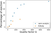 |
Fig. 7. Number of ejections as a function of the effective quality factor of the planet. Each dot is representative of a run of 100 simulations done with the same value of Q. We observe that the number of ejections using the semi-analytic model is greater than using the N-body. The first reason is that the percentages are computed with all simulations considered, smooth evolutions included. The difference then gets more and more pronounced as the number of smooth evolutions also increases with Q for the N-body code (Table 4), but stays rather low for the semi-analytic simulations. The reason for such differences is probably that the rates of mean longitudes are not properly modelled when we average out all the terms except the resonant ones and such bias appears during the resonance where mean longitudes play an important role. Also for chaotic simulations, the averaged equations are truncated to the fourth power, meaning that they are not suited for high eccentricities. Iapetus nearly never survives if its eccentricity grows over 0.25 during the resonance. Therefore the threshold for the semi-analytic code was set to 0.25 for Iapetus to be considered ejected. |
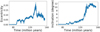 |
Fig. 8. Example of a simulation showing post-resonance eccentricity and inclination compatible with Iapetus’ actual orbit. Here, the resonance is crossed 90 millions years after the start of the simulation. As Iapetus evolves chaotically during the crossing, its eccentricity rises over 0.2, while the tilt also increases to over 10°. On such an orbit, Iapetus is expected to get ejected, but at the end, before getting out of the resonance, the eccentricity decreases to 0.05 while the tilt stays well over the value we observe today. |
6. Discussion on the model
We have left aside the gravitational effect of the outer planets, but it is worth asking if it is a fair negligence. Jupiter evolves close to 5:2 mean motion commensurability with Saturn and plays a major role in its secular motion around the Sun. One of the main aspects of this perturbation is a secular change of Saturn’s eccentricity with a period of around 50 000 years (Murray & Dermott 2000). If we go back to Eq. (16), we see that the Laplace plane equilibrium has a dependency on the planet’s eccentricity (alias the Sun’s eccentricity in our model). However, although the Laplace plane equilibrium will change at the same frequency as the Sun’s eccentricity, the free inclination will still preserve a constant tilt to it.
The precession of the spin axis of Saturn was also a subject of concern to obtain the correct dynamics. We have taken it into consideration and implemented a code where both satellites orbit a precessing Saturn. Numerical simulations show that the satellite orbital planes will follow the precessing spin pole of the planet. This dynamic was also studied in the pioneer paper Goldreich (1965b) in which the perturbing effects were those of the precession of the spin axis of the planet and its flattening. The slow precession of Saturn (French et al. 2017) acts like an adiabatic process that does not alter the mutual perturbation between satellites.
Hyperion was also integrated with the other bodies to monitor any significant changes to its orbit and to the 4:3 mean motion resonance with Titan. No radical changes were detected during the 5:1 crossing between Titan and Iapetus. Hyperion would have therefore easily survived a triple commensurability with Titan and Iapetus; this result was already outlined in a previous study (Ćuk et al. 2013). We have also found that the commensurability is preserved regardless of the tidal migration.
In this study we have neglected tides acting on satellites but the question of damping the eccentricity of Iapetus arises here because of the great number of simulations showing high post-resonance eccentricities. For tides acting on a satellite, we have (Malhotra 1991)
 (32)
(32)
where k2,s and Qs are the Love number and the quality factor of the satellite, ms and Rs its mass and radius and mS the mass of Saturn. Such an equation admits an evolution timescale, in years, of
 (33)
(33)
which is well over the age of the solar system. Therefore, tides are too weak to damp the satellite’s eccentricity during its excitation. Still it is worth mentioning that stronger tidal damping of Iapetus’ eccentricity should occur through its secular coupling to Titan’s eccentricity (Nesvorný et al. 2014).
The semi-analytic model was also tested using quadrupole precision floating-point numbers and has shown similar outcomes to simulations made in double precision. Also more solar terms involving the Sun’s mean longitude were added as well as terms associated to the relation 10λIapetus − 2λTitan, but no real new behaviour appeared.
7. Conclusion
We have simulated a mean motion resonance crossing between Titan and Iapetus using direct N-body integration as well as averaged equations of motion. Both methods have shown similar behaviour regarding statistical outcomes for the fate of Iapetus. The averaged equations were used to study the crossing for slow migration rates of Titan and, as for the N-body code, showed a large number of ejections of Iapetus if Q was set to a value over 2000. A fast migration rate would preserve Iapetus’ eccentricity under a few percent, without however disturbing its orbital tilt to the Laplace plane. The rise of eccentricity is generally consistent with today’s value of around 3% for Q between 20 and 2000. Those values are consistent with quality factors found for the icy satellites in Lainey et al. (2012, 2017). Simulations with Q set over 2000 have shown a majority of unwanted scenarios such as ejections or smooth evolutions, therefore Q = 2000 sets a lower limit to the tidal energy dissipation acting inside Saturn. A quality factor over 100 is necessary to raise Iapetus’ free inclination to values approaching the tilt to the Laplace plane observed today. The tilt mainly stays beneath 5°, but a few simulations have shown tilts to the Laplace plane reaching 8° and beyond with an eccentricity relatively small. Therefore, although the eccentricity excitation of Iapetus is easy to obtain with this resonance, increasing the free inclination is harder. However, a few simulations (less than 1%) have shown some compatibility with Iapetus’ orbit, therefore the scenario that Titan is responsible for Iapetus’ orbit with this past resonance is plausible (cf. 8). A quality factor at Titan’s frequency between 100 and 2000 implies that the resonance crossing happened between 40 million and 800 billion years ago. This result reinforces the idea of strong energy dissipation inside Saturn.
Gm⊙ should be replaced rigorously by  , but
, but  so
so  .
.
The Titan-Sun semi-major axis ratio is 8.5 × 10⁻⁴ and the one concerning Iapetus and the Sun is 2.5 × 10⁻³.
For example, one simulation reaches 10.6° with almost 0.1 eccentricity while another shows 4.8° and 0.038 in eccentricity.
Acknowledgments
The authors acknowledge the support of the contract Prodex CR90253 from the Belgian Science Policy Office (BELSPO). This study is part of the activities of the ISSI Team The ENCELADE Team: Constraining the Dynamical Timescale and Internal Processes of the Saturn and Jupiter Systems from Astrometry. Computational resources have been provided by the Consortium des Équipements de Calcul Intensif (CÉCI), funded by the Fonds de la Recherche Scientifique de Belgique (F.R.S.-FNRS) under Grant No. 2.5020.11. Also, this work was granted access to the HPC resources of MesoPSL financed by the Region Ile de France and the project Equip@Meso (reference ANR-10-EQPX-29-01) of the programme Investissements d’Avenir supervised by the Agence Nationale pour la Recherche. VL’s research was supported by an appointment to the NASA Postdoctoral Program at the NASA Jet Propulsion Laboratory, Caltech, administered by the Universities Space Research Association under contract with NASA. The authors are indebted to all participants of the ISSI Encelade team.
References
- Brouwer, D., & Clemence, G. 1961, Methods of Celestial Mechanics (Academic Press). [Google Scholar]
- Colombo, G., Franklin, F. A., & Shapiro, I. I. 1974, AJ, 79, 61 [NASA ADS] [CrossRef] [Google Scholar]
- Cooper, N. J., Lainey, V., Meunier, L.-E., et al. 2018, A&A, 610, A2 [NASA ADS] [CrossRef] [EDP Sciences] [Google Scholar]
- Ćuk, M., Dones, L., & Nesvorný, D. 2013, ApJL, submitted [arXiv:1311.6780]. [Google Scholar]
- Efroimsky, M. 2012, A&A, 544, A133 [NASA ADS] [CrossRef] [EDP Sciences] [Google Scholar]
- Efroimsky, M., & Lainey, V. 2007, J. Geophys. Res. (Planets), 112, E12003 [Google Scholar]
- Everhart, E. 1974, Celestial Mech., 10, 35 [NASA ADS] [CrossRef] [Google Scholar]
- Everhart, E. 1985, in Dynamics of Comets: Their Origin and Evolution, Proceedings of IAU Colloq. 83, held in Rome, Italy, June 11–15, 1984, eds. A. Carusi, & G. B. Valsecchi, Astrophysics and Space Science Library (Dordrecht: Reidel), 115, 185 [Google Scholar]
- French, R. G., McGhee-French, C. A., Lonergan, K., et al. 2017, Icarus, 290, 14 [NASA ADS] [CrossRef] [Google Scholar]
- Fuller, J., Luan, J., & Quataert, E. 2016, MNRAS, 458, 3867 [NASA ADS] [CrossRef] [Google Scholar]
- Goldreich, P. 1965a, MNRAS, 130, 159 [NASA ADS] [Google Scholar]
- Goldreich, P. 1965b, AJ, 70, 5 [NASA ADS] [CrossRef] [Google Scholar]
- Goldreich, P., & Soter, S. 1966, Icarus, 5, 375 [Google Scholar]
- Greenberg, R. 1973, AJ, 78, 338 [NASA ADS] [CrossRef] [Google Scholar]
- Guenel, M., Mathis, S., & Remus, F. 2014, A&A, 566, L9 [NASA ADS] [CrossRef] [EDP Sciences] [Google Scholar]
- Kaula, W. M. 1964, Rev. Geophys. Space Phys., 2, 661 [Google Scholar]
- Lainey, V., Karatekin, Ö., Desmars, J., et al. 2012, ApJ, 752, 14 [Google Scholar]
- Lainey, V., Jacobson, R. A., Tajeddine, R., et al. 2017, Icarus, 281, 286 [NASA ADS] [CrossRef] [Google Scholar]
- Malhotra, R. 1991, Icarus, 94, 399 [NASA ADS] [CrossRef] [Google Scholar]
- Mignard, F. 1980, Moon and Planets, 23, 185 [NASA ADS] [CrossRef] [Google Scholar]
- Murray, C., & Dermott, S. 2000, Solar System Dynamics (Cambridge University Press). [CrossRef] [Google Scholar]
- Nesvorný, D., Vokrouhlický, D., Deienno, R., & Walsh, K. J. 2014, AJ, 148, 52 [NASA ADS] [CrossRef] [Google Scholar]
- Rein, H., & Spiegel, D. S. 2015, MNRAS, 446, 1424 [NASA ADS] [CrossRef] [Google Scholar]
- Remus, F., Mathis, S., & Zahn, J.-P. 2012a, A&A, 544, A132 [NASA ADS] [CrossRef] [EDP Sciences] [Google Scholar]
- Remus, F., Mathis, S., Zahn, J.-P., & Lainey, V. 2012b, A&A, 541, A165 [NASA ADS] [CrossRef] [EDP Sciences] [Google Scholar]
- Remus, F., Mathis, S., Zahn, J.-P., & Lainey, V. 2015, A&A, 573, A23 [NASA ADS] [CrossRef] [EDP Sciences] [Google Scholar]
- Roy, A. E., & Ovenden, M. W. 1954, MNRAS, 114, 232 [NASA ADS] [CrossRef] [Google Scholar]
- Tremaine, S., Touma, J., & Namouni, F. 2009, AJ, 137, 3706 [NASA ADS] [CrossRef] [Google Scholar]
- Tsiganis, K., Gomes, R., Morbidelli, A., & Levison, H. F. 2005, Nature, 435, 459 [NASA ADS] [CrossRef] [PubMed] [Google Scholar]
- Ward, W. R. 1981, Icarus, 46, 97 [NASA ADS] [CrossRef] [Google Scholar]
- Zahn, J. P. 1966, Annales d’Astrophysique, 29, 313 [Google Scholar]
All Tables
All Figures
|
Fig. 1. Motion of Iapetus plane over 10 000 years. Both the inclination and the longitude of the ascending node oscillate around the fixed values of the Laplace plane with a period of around 3200 years. Here, and for the rest of this work, the reference plane is the equator of Saturn. The figure comes from a simulation done with all the major satellites of Saturn (Mimas, Enceladus, Tethys, Dione, Rhea, Titan, Hyperion, Iapetus), the Sun, and the effect of the flattening of Saturn. The angular elements of the Laplace plane are approximately 15° for the inclination and 225° for the ascending node. The initial conditions are those of the J2000 epoch taken from JPL ephemeris, Horizon (SAT 389.14). |
| In the text | |
|
Fig. 2. Level curve of the Hamiltonian from Eq. (7). Orbital plane elements will follow the solid lines. One can distinguish four different kinds of equilibrium: one for retrograde orbits, two for polar orbits, and the one we are interested in, for relatively low inclination. The latter gives us Ω = Ω⊙ and both ascending nodes of Iapetus and Titan oscillate around it. Equation (12) and Table 2 give an inclination of the local Laplace plane of Titan around 0.62°. |
| In the text | |
|
Fig. 3. Tilt of Iapetus’ local Laplace plane to Saturn’s equator as a function of Iapetus’ semi-major axis. Here |
| In the text | |
|
Fig. 4. Smooth evolutions of the eccentricity and the inclination coming from two different simulations. On the left, the eccentricity of Iapetus growths smoothly after both satellites enter the resonance, while the tilt stays constant. The right figure depicts the evolution of the inclination with respect to the Laplace plane. For this simulation, the eccentricity does not change. |
| In the text | |
|
Fig. 5. Example of a resonance crossing with Q = 50 using the N-body code. The obvious effect of the resonance is here a “kick” in both eccentricity and free inclination. |
| In the text | |
|
Fig. 6. Example figures of outputs obtained from our simulations. In this example we clearly distinguish a regular evolution before the resonance, a chaotic resonance crossing, and finally regular dynamics after the resonance. In this specific example, the eccentricity increase is around 0.035 and the tilt has grown to around 4.5. These two figures were taken from a run of 100 simulations using the semi-analytic model with Q = 200. |
| In the text | |
|
Fig. 7. Number of ejections as a function of the effective quality factor of the planet. Each dot is representative of a run of 100 simulations done with the same value of Q. We observe that the number of ejections using the semi-analytic model is greater than using the N-body. The first reason is that the percentages are computed with all simulations considered, smooth evolutions included. The difference then gets more and more pronounced as the number of smooth evolutions also increases with Q for the N-body code (Table 4), but stays rather low for the semi-analytic simulations. The reason for such differences is probably that the rates of mean longitudes are not properly modelled when we average out all the terms except the resonant ones and such bias appears during the resonance where mean longitudes play an important role. Also for chaotic simulations, the averaged equations are truncated to the fourth power, meaning that they are not suited for high eccentricities. Iapetus nearly never survives if its eccentricity grows over 0.25 during the resonance. Therefore the threshold for the semi-analytic code was set to 0.25 for Iapetus to be considered ejected. |
| In the text | |
|
Fig. 8. Example of a simulation showing post-resonance eccentricity and inclination compatible with Iapetus’ actual orbit. Here, the resonance is crossed 90 millions years after the start of the simulation. As Iapetus evolves chaotically during the crossing, its eccentricity rises over 0.2, while the tilt also increases to over 10°. On such an orbit, Iapetus is expected to get ejected, but at the end, before getting out of the resonance, the eccentricity decreases to 0.05 while the tilt stays well over the value we observe today. |
| In the text | |
Current usage metrics show cumulative count of Article Views (full-text article views including HTML views, PDF and ePub downloads, according to the available data) and Abstracts Views on Vision4Press platform.
Data correspond to usage on the plateform after 2015. The current usage metrics is available 48-96 hours after online publication and is updated daily on week days.
Initial download of the metrics may take a while.