| Issue |
A&A
Volume 619, November 2018
|
|
|---|---|---|
| Article Number | A150 | |
| Number of page(s) | 17 | |
| Section | Planets and planetary systems | |
| DOI | https://doi.org/10.1051/0004-6361/201833709 | |
| Published online | 16 November 2018 | |
Activity induced variation in spin-orbit angles as derived from Rossiter–McLaughlin measurements
1
Institut für Astrophysik, Georg-August Universität Göttingen,
Friedrich-Hund-Platz 1,
37077
Göttingen,
Germany
e-mail: moshagh@astro.physik.uni-goettingen.de
2
Instituto de Astrofísica e Ciências do Espaço, Universidade do Porto, CAUP, Rua das Estrelas,
4150-762
Porto,
Portugal
3
University of Birmingham,
Edgbaston,
Birmingham,
B15 2TT,
UK
4
Space Sciences, Technologies and Astrophysics Research (STAR) Institute, Université de Liège, Allée du 6 Août 17, Bat. B5C,
4000
Liège,
Belgium
5
European Southern Observatory, Alonso de Cordova 3107, Vitacura Casilla
19001,
Santiago 19,
Chile
6
Departamento de Física e Astronomia, Faculdade de Ciências, Universidade do Porto, Rua do Campo Alegre,
4169-007
Porto,
Portugal
7
IMCCE, Observatoire de Paris, UPMC University Paris 6, PSL Research University,
Paris,
France
8
Universidad de Buenos Aires, Facultad de Ciencias Exactas y Naturales,
Buenos Aires
1428,
Argentina
9
CONICET – Universidad de Buenos Aires, Instituto de Astronomía y Física del Espacio (IAFE),
Buenos Aires
1428,
Argentina
10
Astrophysics Group, Cavendish Laboratory, J. J. Thomson Avenue, Cambridge CB3 0HE,
UK
11
Hamburg Observatory, Hamburg University,
Gojenbergsweg 112,
21029
Hamburg,
Germany
12
Max Planck Institute for Astronomy,
Königstuhl 17,
69117
Heidelberg,
Germany
13
Observatoire de Genève, Université de Genève,
51 chemin des Maillettes,
1290
Versoix,
Switzerland
Received:
25
June
2018
Accepted:
17
August
2018
One of the most powerful methods used to estimate sky-projected spin-orbit angles of exoplanetary systems is through a spectroscopic transit observation known as the RossiterMcLaughlin (RM) effect. So far mostly single RM observations have been used to estimate the spin-orbit angle, and thus there have been no studies regarding the variation of estimated spin-orbit angle from transit to transit. Stellar activity can alter the shape of photometric transit light curves and in a similar way they can deform the RM signal. In this paper we present several RM observations, obtained using the HARPS spectrograph, of known transiting planets that all transit extremely active stars, and by analyzing them individually we assess the variation in the estimated spin-orbit angle. Our results reveal that the estimated spin-orbit angle can vary significantly (up to ~42°) from transit to transit, due to variation in the configuration of stellar active regions over different nights. This finding is almost two times larger than the expected variation predicted from simulations. We could not identify any meaningful correlation between the variation of estimated spin-orbit angles and the stellar magnetic activity indicators. We also investigated two possible approaches to mitigate the stellar activity influence on RM observations. The first strategy was based on obtaining several RM observations and folding them to reduce the stellar activity noise. Our results demonstrated that this is a feasible and robust way to overcome this issue. The second approach is based on acquiring simultaneous high-precision short-cadence photometric transit light curves using TRAPPIST/SPECULOOS telescopes, which provide more information about the stellar active region’s properties and allow a better RM modeling.
Key words: planets and satellites: fundamental parameters / planets and satellites: detection / stars: activity / starspots / techniques: radial velocities / techniques: photometric
© ESO 2018
1 Introduction
Understanding the orbital architecture of exoplanetary systems is one of the main objectives of exoplanetary surveys, in order to provide new strong constraints on the physical mechanisms behind planetary formation and evolution. The sky-projected spin-orbit angle (hereafter spin-orbit angle λ)1 is one of the most important parameters of the orbital architecture of planetary systems. According to the core-accretion paradigm of planet formation, planets should form on aligned orbits λ ~ 0 (Pollack et al. 1996; and see a comprehensive review in Dawson & Johnson 2018, and references therein), as observed in the case of the solar system. Planetary evolution mechanisms such as disk migration predict that planets should maintain their primordial spin-orbit angle, but the dynamical interactions with a third body and tidal migration could alter the spin-orbit angle (see a comprehensive review in Baruteau et al. 2014, and references therein). Moreover, several studies have shown that the misalignment of a planet could be primordial considering the disks being naturally and initially misaligned (e.g., Batygin 2012; Crida & Batygin 2014). In this context, the measurement of spin-orbit angles under a wide range of host and planet conditions (including multiple transiting planets) is extremely important in order to obtain feedback on modeling.
As a star rotates, the part of its surface that rotates toward the observer is blueshifted and the part that rotates away is redshifted. During the transit of a planet, the corresponding rotational velocity of the portion of the stellar disk that is blocked by the planet is removed from the integration of the velocity over the entire star, creating a radial velocity (RV) signal known as the Rossiter–McLaughlin (RM) effect (Holt 1893; Rossiter 1924; McLaughlin 1924). The RM observation is the most powerful and efficient technique for estimating the spin-orbit angle λ of exoplanetary systems or eclipsing binary systems (e.g., Winn et al. 2005; Hébrard et al. 2008; Triaud et al. 2010; Albrecht et al. 2012, and a comprehensive review in Triaud 2017, and references therein). The number of spin-orbit angle λ measurements has dramatically increased over the past decade (200 systems to date)2, and have revealed a large number of unexpected systems, which include planets on highly misaligned (e.g., Triaud et al. 2010; Albrecht et al. 2012; Santerne et al. 2014), polar (e.g., Addison et al. 2013), and even retrograde orbits (e.g., Bayliss et al. 2010; Hébrard et al. 2011).
The contrast of active regions (i.e., stellar spots, plages, and faculae) present on the stellar surface during the transit of an exoplanet alter the high-precision photometric transit light curve (both outside and inside transit) and lead to an inaccurate estimate of the planetary parameters (e.g., Czesla et al. 2009; Sanchis-Ojeda & Winn 2011; Sanchis-Ojeda et al. 2013; Oshagh et al. 2013b, 2015a,b; Barros et al. 2013; Ioannidis et al. 2016). Since the physics and geometry behind the transit light curve and the RM measurement are the same, the RM observations are expected to be affected by the presence of stellar active regions in a similar way. Furthermore, the inhibition of the convective blueshift inside the active regions can induce extra RV noise on the RM observations, which is absent in the photometric transit observation.
Boldt et al. (in prep.) demonstrate, using simulations, that unocculted stellar active regions during the planetary transit influence the RV slope of out-of-transit in RM observations (due to a combination of contrast and stellar rotation) and leads to an inaccurate estimate of the planetary radius; however, their influence on the estimated λ was negligible. On the other hand, Oshagh et al. (2016) demonstrated that the occulted stellar active regions can lead to quite significant inaccuracies in the estimation of spin-orbit angle λ (up to ~ 30° for Neptune-sized planets and up to ~15° for hot Jupiters), which is much larger than the typical error bars on the λ measurement, especially in the era of high-precision RV measurements like those provided by HARPS (Mayor et al. 2003), HARPS-N (Cosentino et al. 2012), CARMENES (Quirrenbach et al. 2014), and that will be provided by ESPRESSO (Pepe et al. 2014).
In almost all (all could be an overstated or exaggerated statement) studies of RM observations, only one RM observation during a single transit was acquired, and single-epoch RM observations were used to estimate the spin-orbit angle λ of the systems. The main reason for this is the high telescope pressure and oversubscription on high-precision spectrographs that makes requesting for several RM observations of same targets inaccessible. Therefore, the lack of multiple RM observations has not permitted us to explore possible contamination on the estimated λ from the stellar activity.
In this paper we assess the impact of stellar activity on the spin-orbit angle estimation by observing several RM observations of known transiting planets which all transit extremely active stars. We organize our paper as follows. We describe our targets’ selection and their observations in Sect. 2. In Sect. 3 we define our fitting procedure to estimate the spin-orbit angles, and also present its result. We investigate the possibility of mitigating the influence of stellar activity on RM observations by combining several RM observations in Sect. 4. In Sect. 5 we present the simultaneous photometric transit observation with our RM observation and we discuss the advantages of having simultaneous photometric transit observation in eliminating stellar activity noise in RM observations. In Sect. 6, we discuss possible contamination from other sources of stellar noise that affect our observations, and conclude in Sect 7.
2 Observations and data reduction
2.1 Target selection
Our stars were selected following four main criteria:
the star should have a known transiting planet;
the planet host star should be very active (e.g., the published photometric transit light curves clearly show large stellar spots’ occultation anomalies);
at least one RM measurement of the planet has been observed (preferably with the HARPS spectrograph as we use HARPS observations in our study) to ensure the feasibility of detecting the RM signal;
the transiting planet should have several observable transits from the southern hemisphere during the period from March 2017 to October 2017 (this criterion is to ensure observability).
Our criteria resulted in the selection of six transiting exoplanets, namely, WASP-6b, WASP-19b, WASP-41b, WASP-52b, CoRoT-2b, and Qatar-2b. Their published transit light curves have indicated the presence of stellar spots on their surfaces with a filling factor of 6, 8, 3, 15, 16, and 4%, respectively (Nutzman et al. 2011; Tregloan-Reed et al. 2015; Sedaghati et al. 2015; Southworth et al. 2016; Mancini et al. 2017; Dai et al. 2017). Most of them also have at least one observed RM with HARPS (Bouchy et al. 2008; Gillon et al. 2009; Hellier et al. 2011; Neveu-VanMalle et al. 2016), except for Qatar-2, which has one observed RM with the HARPS-N spectrograph (Esposito et al. 2017) and for WASP-52, which has one observed RM with the SOPHIE spectrograph (Hébrard et al. 2013).
We list all the planetary and stellar parameters of our targets collected from the literature and that are necessary for our analysis in Table 1.
Planetary and stellar parameters of our targets.
2.2 HARPS observation
Our program was allocated 60 h on the HARPS spectrograph, mounted on the ESO 3.6 m telescope at La Silla observatory (Mayor et al. 2003), to carry out high-precision RV measurements during three transits of each of our targets (under ESO programme ID: 099.C-0093, PI: M. Oshagh). The main aim of our program was to measure the spin-orbit angle λ from individual RM observation of each target, by having multiple λ measurements for each target, and to quantify the changes in the measured λ from transit to transit.
Thanks to the time-sharing scheme on HARPS with several other observing programs we were able to spread our 60 h (equivalent to six nights) over a large fraction of the semester and obtain observations during several nights in which transits occur. Due to bad weather we lost almost 35% of our allocated time, thus we could not obtain three RM observations for all of our targets. We summarize the number of RM observations collected for each target and the nights in Table 2. To overcome the shortage of several RM observations for some of our targets, we decided to collect the publicly available RM observations, preferably obtained with HARPS, of those targets (called extra RM). The extra RM observations, their observed dates, and the spectrograph are also listed in Table 2.
The RM observation for each transit started at least one hour before the start of the transit and lasted until one hour after the transit ended. The exposure times range from 900 to 1200 s, ensuring a constant signal-to-noise ratio. All our targets throughout the observations remained above airmass 1.8 (X <1.8). The spectra were acquired with simultaneous Fabry–Perot spectra on fiber B for simultaneous wavelength reference, and were taken with the detector in fast-readout mode to minimize overheads and increase the total integration time during transit.
The collected HARPS spectra in our study were reduced using the HARPS Data Reduction Software (DRS; Pepe et al. 2002; Lovis & Pepe 2007). The spectra were cross-correlated with masks based on their stellar spectral type. As output the DRS provides the RVs and associated error.
Summary of RM observation nights and the simultaneous photometry.
2.3 TRAPPIST/SPECULOOS observations
We obtained additional simultaneous high-precision photometric transit observations with some of our RM observations using TRAPPIST-South3 (Gillon et al. 2011; Jehin et al. 2011), and one of the SPECULOOS4 Southern Observatory telescopes (Gillon 2018; Burdanov et al. 2017). TRAPPIST-South is a 60 cm (F/8) Ritchey–Chrétien telescope installed by the University of Liège in 2010 at the ESO La Silla Observatory in the Atacama Desert in Chile. The SPECULOOS Southern Observatory is a facility composed of four robotic Ritchey–Chrétien (F/8) telescopes of 1 m diameter currently being installed at the ESO Paranal Observatory (PI of both telescopes: M. Gillon). The main objective of obtaining simultaneous high-precision and high-cadence photometric transit light curves was to assist us in identifying the presence of occultations of active regions by the planet during the transits. We listed the nights on which simultaneous photometric transits were collected in Table 2.
The observation for each transit started at least one hour before the start of the transit and lasted until one hour after the transit ended. The TRAPPSIT and SPECULOOS observations were acquired in V band and Sloan g’, respectively. The exposure times range from 10 to 35 s.
Data reduction consisted of standard calibration steps (bias, dark, and flat-field corrections) and subsequent aperture photometry in IRAF/DAOPHOT (Stetson 1987). Comparison stars and aperture size were selected manually to ensure the best photometric quality in terms of the flux standard deviation of check stars, i.e., non-variable stars similar in terms of magnitude and color to the target star.
3 Variation of spin-orbit angle
In this section we aim to determine the changes in measured spin-orbit angle λ estimated from individual RM observations for a sample of exoplanets.
3.1 RM model
To estimate the spin-orbit angle λ from RM observations, we use the publicly available code ARoME5 (Boué et al. 2012), which provides an analytical model to compute the RM signal, and is optimized for the spectrographs that utilize the CCF-based approach to estimate RVs (such as HARPS). ARoME requires as input parameters the width of a non-rotating star which can be considered as the instrumental broadening profile (β0), width of the best Gaussian fit to out-of-transit CCF (σ0), stellar macroturbulence (ζ), stellar radius (R⋆), projected stellar rotational velocity vsini, stellar quadratic limb darkening coefficients (u1 and u2), planetary semimajor axis (a), orbital period of planet (P), planet-to-star radius ratio (Rp∕R⋆), orbital inclination angle (i), and the spin-orbit angle λ in order to calculate the RM signal.
Brown et al. (2017) performed a comparison study between ARoME and other RM modeling tools, and reached the conclusion that ARoME consistently underestimates vsini when compared to other models. Although vsini differed, the estimated λ were in strong agreement for all the models. Moreover, ARoME is the only code which is publicly available, and we are only interested in estimating λ and in its variation, thus we decided to use the ARoME tool for our analysis.
3.2 Fitting RM observation
As the first step of our analysis we carry out a least-squares linear fit to the out-of-transit RV data of each observed RM observations for each planet, and remove the linear trend. The main purpose of this is to eliminate the RV contribution from the Keplerian orbit (which we assume to be linear for the period of observations)6, the systematics, and also the stellar activity which induces RV slopes to the out-of-transit RV data points (Boldt et al., in prep.). After the linear trend is removed, we fit individual RM observation with the ARoME model.
In our fitting procedure we consider the spin-orbit angle (λ), projected stellar rotational velocity (vsini), and the mid-transit time (T0) as our free parameters. Due to presence of degeneracy between λ and vsini, especially for a low-impact parameter system (Brown et al. 2017), frequently these are the two common free parameters in fitting and analyzing RM signals. Since ARoME generates an RM signal centered around zero time (assuming zero as the mid-transit), we have to remove the mid-transit times (calculated based on the reported ephemeris and orbital period of the planet) from our observation7. Due to the uncertainty on the reported value of the ephemeris and also the possible variation in transit time (due to the presence of an unknown companion in the systems) the calculated T0 might not be very accurate; thus, we decided to leave T0 as the third free parameter. It could be argued that the slope of the out-of-transit trend should be one of our free parameters in the fitting RM, but since Boldt et al. (in prep.) demonstrated that trend removal does have a negligible impact on the spin-orbit angle λ estimation, we decided to fit the slope and remove the trend prior to our RM fitting procedure. Nonetheless, to evaluate our choice, we explore the consequences of leaving the slope as an extra free parameter in our fitting procedure in Appendix A. The result of that test indicates that the impact is negligible on the other parameters, which support our choice.
The rest of the parameters required in ARoME, such as stellar radius (R⋆), quadratic limb darkening coefficients of the star (u1 and u2), the semimajor axis of the planet (a), the orbital period of planet (P), and the planetary orbital inclination angle (i), are fixed to their reported values in the literature (which are given in Table 1). We also fixed the macro-turbulence velocity of all stars to ζ = 4 km s−1 and fixed the instrumental broadening according to the HARPS instrument profile (β0 = 1.3 km s−1). We would like to note that the macro-turbulence might not be an accurate estimate, but since we are only interested in the variation in λ, the inaccurate macro-turbulence will be the same on all our measured λ. We also evaluate having macro-turbulence as an extra free parameter in our fitting procedure in Appendix B. Its results also demonstrate that the impact is negligible on the other parameters, which supports our choice.We also fixed the width of the Gaussian (σ0) to the width of a Gaussian fit to the CCF of out-of-transit for each star. We note that we have two strong arguments for not letting these parameters be free in our fitting procedure. The first is that we want to have very similar fitting procedures to most of the RM studies, which only use λ and v sin i as free parameters and fix the rest of the parameters to the values obtained from photometric transit. The second reason is based on the small number of data points in each RM observation. Thus, if we consider all these parameters free we would have more free parameters than observations and we might end up withan overfitted model.
The best fit parameters and associated uncertainties in our fitting procedure are derived using a Markov chain Monte Carlo (MCMC) analysis, using the affine invariant ensemble sampler emcee (Foreman-Mackey et al. 2013). The prior on v sin i and T0 are controlled by Gaussianpriors centered on the reported value in the literature and width according to the reported uncertainties, and the prior on λ is also controlled by a uniform (uninformative) prior between ± 180°. We list the selected type of priors and ranges for our free parameters for each target in Table 3.
We randomly initiated the initial values for our free parameters for 30 MCMC chains inside the prior distributions. For each chain we used a burn-in phase of 500 steps, judging the chain to be converged, and then again sampled the chains for 5000 steps. Thus, the results concatenated to produce 150 000 steps. We determined the best fitted values by calculating the median values of the posterior distributions for each parameters, based on the fact that the posterior distributions were Gaussian. The 1σ uncertainties were taken to be the value enclosed in the 68.3% of the posterior distributions.
Details of the priors that we apply during our MCMC analysis.
3.3 Significant variation of spin-orbit angle
Figure 1 shows the posterior distributions in v sin i − λ parameter space of all our targets delivered by the fit to individual RM obtained during different transits on different nights. We listed the best fitted values of λ and v sin i from individual RM observations in Table 4. We found that the estimated spin-orbit angle λ of an exoplanet can be significantly altered (up to 42°) from transitto transit due to variation in the configurations of the stellar active regions on different nights (mainly as a consequence of the stellar rotation and also the evolution of the stellar active regions)8. The estimated λ variation was larger than the simulation’s result we described in a previous work, which suggested a variation of up to 15° for hot Jupiters (Oshagh et al. 2016). The uncertainty on the estimated λ also varies significantly from transit to transit.
The estimated vsini from the ARoME fit, as mentioned in Brown et al. (2017), are usually underestimated in comparison to their literature values; however, our goal here is not to measure their value accurately but to evaluate their variation from transit to transit. Our results depict a deviation of estimated v sin i from transit to transit; however, for most of the cases the variations are in the uncertainty ranges, and thus could be considered insignificant. However, we would like to note again that since ARoME generally underestimates vsini this result should be taken with a grain of salt.
The fitted transit time T0 for all of our targets coincided with the respective calculated value (based on assuming an unperturbed Keplerian orbit with fixed periodic planetary orbit and according to reported ephemeris). Therefore, we conclude that our observations do not exhibit any signs of transit time variation for any of our targets. However, we would like to note that there might still be transit timing variation in our targets, but we could not detect it due to the small number of points in our RM observations, which prevented us from achieving high-precision transit time estimations.
We present each individual RM observation (obtained during different nights) for each of our targets with their best fitted model in Figs. C.1–C.6.
Best fitted values for λ and v sin i obtained from each RM observations.
4 Probing the correlations between log R’HK and spin-orbit angle variation
In this section we assess the presence of any meaningful correlation between the amplitude of the variation of spin-orbit angle (largest variation Δ λ) and measured stellar activity indicator log  9. The values of log
  s were delivered as a by-product of DRS (as described in Lovis et al. 2011). We calculated the mean of measured log
  s for our stars during our observation, and used the mean value as the measured log
  . We also measured the standard deviation of log
  s and used it as the uncertainty on the measured
  . The value of
 by itself canalso provide information about the variation in magnetic activity of stars during our observation, due to a stellar active region either appearing or disappearing or to the occultation of the active region by a transiting planet.
We inspected the presence of a correlation based on the Spearman’s rank-order correlation coefficient (ρ)10. We evaluated the significance of correlation using the Bayesian approach described in Figueira et al. (2016). The posterior distribution of ρ indicates the range of ρ values that is compatible with the observations.
Figure 2, top panel, presents the correlations between Δ λ and log  . We note that Qatar-2, due to its faintness (V = 13.3) and low signal-to-noise ratio in the region of spectrum in which log
  is estimated, has only one estimated log
  ; therefore, it was impossible to measure its
  . As this figure shows, there is no meaningful correlation between the measured value of Δ λ and log
  . Figure 2, bottom panel, displays the correlations between Δ λ and
  , which show an anti-correlation but not a significant correlation. We note that in this plot we discarded Qatar-2.
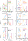 |
Fig. 1 Posterior probability distributions in vsini − λ parameter space of all our targets obtained from the fit to individual RM observations obtained at different transits and on different nights. Each panel shows different planetary system, and in each panel different colors correspond to the different nights on which the RM observation were performed. The purple dashed line displays the reported value in the literature. B+08: Bouchy et al. (2008), H+11: Hellier et al. (2011), N+16: Neveu-VanMalle et al. (2016), G+09: Gillon et al. (2009), H+13: Hébrard et al. (2013), E+17: Esposito et al. (2017). |
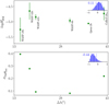 |
Fig. 2 Top panel: correlations between Δλ and log |


5 Folding several RM observations
The most logical approach for eliminating the effect of stellar activity on RM observations, and thus minimizing its impact on the estimated spin-orbit angle λ, is to obtain several RM observations and combine and fold them. This is based on the fact that the configuration of the stellar active region evolves from transit to transit, but the planetary RM signal remains constant; thus, averaging several RM observations will average out the activity noise and increase the planetary RM signal-to-noise ratio. Therefore, in this section we fold all the observed RM observations for each planet (analyzed in the previous section), and try to repeat the fitting procedure to estimate more accurately the spin-orbit angle λ and the host star v sin i.
In order to fold all the available RM observations for each target, we utilize the best fitted transit time (T0) obtained in the previous section. Therefore, in our fitting procedure we no longer leave the transit time as a free parameter, thus λ and v sin i are our only free parameters.
Figure 3 presents the posterior distributions from the fit to folded RM observations of all of our targets, and displays the best fitted values for λ and vsini and their associated 1σ uncertainties. We summarized the best fitted values in Table 5. Moreover, in Table 5 we also list the estimated values of λ for our targets, which were estimated from an independent method of recurring starspot occultationsin photometric transit light curve observations. The comparison between our estimated λ from folded RM observations and those measured from recurring starspot occultations (both presented in Table 5) reinforce that the strategy of folding RM observations adequately eliminates the stellar activity effect, and provides an accurate estimate of λ. We present the folded RM observations for each of our targets and their best fitted model in Fig. 4.
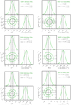 |
Fig. 3 Posterior probability distributions in vsini − λ parameter space of all our targets obtained from the fit to the folded RM observations. Each panel shows different planetary system. The black dashed line displays median values of the posterior distributions, and the 1σ uncertainties taken to be the value enclosed in the 68.3% of the posterior distributions are shown with the black dotted line. |
Best fitted values for λ and v sin i obtained from folded RM observations.
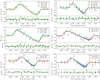 |
Fig. 4 Folded RM observations of our targets during several nights. The green line shows the best fitted RM model and blue region shows the zone where 68% of the model solutions reside. In each panel the residuals are shown in the bottom panel. |
6 Simultaneous photometric transit light curve and RM observations
Photometric transit observations can usually be acquired on much shorter exposure times than RM observations11, and thus could lead to the easier and clearer detection of the occultation of active regions during the transit of an exoplanet. We obtained five simultaneous photometric transit observations with our RM observations, four with the TRAPPSIT telescope and one with SPECULOOS. All the photometric transit light curves clearly indicated the presence of active regions’ crossing. Thus, the main aim of this section is to assess whether we can have a better RM modeling by having the information from the active region’s crossing event during a photometric transit (which provides information about the size, position, and contrast of active regions).
6.1 Fitting photometric transit anomalies with SOAP3.0
In this section we use the publicly available tool SOAP3.0. This tool has the capability of simulating a transiting planet and a rotating star covered with active regions, and delivers photometric and RV variation signals. SOAP3.0 takes into account not only the flux contrast effect in these regions, but also the RV shift due to inhibition of the convective blueshift inside these regions. SOAP3.0 also takes into account the occultation between the transiting planet and active regions in its calculation of transit light curve and RM.
We use SOAP3.0 to obtain the best fitted model to the photometric transit light curves and then compare the corresponding RM of the best fitted model with the observed RM observations. Because of the slowness of SOAP3.0, due to its numerical nature in comparison to the analytical nature of ARoME, performing an MCMC approach using SOAP3.0 is not feasible. Therefore, we decided to perform a  minimization using SOAP3.0 to fit the active region crossing events in the photometric transit light curves. From visual inspection we could identify only three active region crossing events during each observed transit light curve, thus we decided to fix the number of active regions to three. In
  minimization we fixed all the required parameters of stars and planets in SOAP3.0 (the same parameters in Table 1) except for the three active regions’ parameters (filling factor, location, and temperature contrast) and let them vary as free parameters. The range of free parameters which were explored are listed as the spots’ filling factor [0.1%:20%], latitude [− 90°: + 90°], longitude [0°:360°], and temperature contrast [0: − Teff].
6.2 Improved RM prediction
As mentioned before, here we intend to compare the corresponding RM of the best fitted model to the transit light curves with the observed RM12. We overplotted the RM counterpart of the best fitted model over the simultaneous observed RM observations for WASP-19b, CoRoT-2b, and Qatar-2b in Figs. 5–7, respectively. This result demonstrated that the RM counterparts coincide much better with the observed RM. As a consequence, the residual between the SOAP3.0 RM whose considered active region crossing is lower than the residual of SOAP3.0 RM without any spot crossing event. To quantify the improvement, we computed the standard deviation of the residual between SOAP3.0 best fit predicted RM and the observed RM, for models ignoring stellar spots and for models taking them into account. All standard deviations are listed in Table 6, and they all support the improvement in the RM prediction.
It is worth mentioning that a strong degeneracy exists between the parameters of the stellar active regions; for instance, different filling factor, position, and contrast could produce very similar photometric signatures while generating completely different RV signals. Therefore, we have to clarify our best fitted model to the photometric transit light curves, and also the best fitted value for the active regions’ parameters might not correspond to accurate values, although they more closely predict the RM observation than considering no active region occultation.
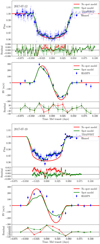 |
Fig. 5 Simultaneous photometric transit and RM observation of CoRoT-2b on the night of 12 July 2017 (top panels) and on night thenight of 19 July 2017 (bottom panels). The dark blue square represents the binned TRAPPIST photometric observations, and the dark blue filled circle the HARPS RM observation. The red line is the SOAP3.0 model without considering any stellar active regions. The green lines are the SOAP3.0 best fitted model to transit light curve taking into accountthree spots. |
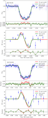 |
Fig. 6 Simultaneous photometric transits and RM observations of WASP-19b on the night of 5 May 2017 (top panels) and on the night of 9 May 2017 (bottom panels). The lines and points are the same as in Fig. 5. |
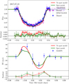 |
Fig. 7 Simultaneous photometric transits and RM observations of Qatar-2b on the night of 10 July 2017. The photometric observationswere obtained from simultaneous observations of TRAPPIST and SPECULOOS. The lines and points are the same as in Fig. 5. |
Standard deviation of the residual between SOAP3.0 predicted RM and observed RM for models that ignore the spot crossing events and for models that take into account spot crossing events.
7 Discussion
Estimation of λ and vsini could be influenced by second-order effects such as the stellar convective blueshift and granulation (Shporer & Brown 2011; Cegla et al. 2016b), the microlensing effect due to the transiting planet’s mass (Oshagh et al. 2013a), the impact of ringed exoplanet on RM signal (Ohta et al. 2009; de Mooij et al. 2017; Akinsanmi et al. 2018), and stellar differential rotation (Albrecht et al. 2012; Cegla et al. 2016a; Serrano et al., in prep.). However, their expected signals in RM observations are different from the active region crossing events. More importantly, all of their signals are constant during several transits; thus, even if they affect the estimation of λ and v sin i, their influence cannot produce variation in the estimated λ. Therefore, of the extensive list of effects above, we can conclude that the variation in the estimated λ could have only originated from the stellar activity noise.
The simulations presented in Oshagh et al. (2016) predicted that the variation in estimated λ could reach up to 15° for hot Jupiters; however, our observational campaign shows a variation that is twice as large. The plausible explanation for this underestimation of variation in the simulation could be that in the simulation the stellar active regions were considered to be similar to the sunspots (e.g., a filling factor of around 1%). However, all the stars in our sample exhibit a much higher level of activity than the Sun, and are covered with much larger stellar spots (filling of stellar spotson the WASP-6, WASP-19, WASP-41, WASP-52, CoRoT-2, and Qatar-2 were 6, 8, 3, 15, 16, and 4%, respectively).
We would like to note that throughout one RM observation the target’s airmass varies, and also from one night to another the mid-transit occurs at different airmass. Moreover, the seeing condition fluctuates from night to night. Therefore, there could be some considerable contribution from airmass and seeing variations which might lead to the variation in observed RM observations. Although this statement is provable, correcting their effect is not a trivial task and beyond the scope of the current study. However, this again points to the fact that having only single-epoch RM observation could be vulnerable to other unaccounted noise sources. Moreover, we would like to suggest obtaining several RM observations of a planet transiting a very inactive star to be able to better explore the seeing and airmass conditions on the estimated λ.
We showed that folding several RM observation could mitigate the impact of stellar active region occultation; however, if RM observation are done on consecutive transits, and are not separated with long time interval from each other, we would like to note that they can be affected by occultation with the same active regions, and thus folding the RM observations will not improve the accuracy of the estimation of λ. Therefore, we suggest obtaining several RM observations with a long time separation compatible with several stellar rotations to ensure that RM observations are affected by the configurations of different active regions.
Our results also highlighted the power of having simultaneous photometric transit observations with RM observations, which provides unique information about the stellar active regions that have been occulted during the transit, and leads to a better elimination of their influence on the observed RM. Thus, in the cases where only one RM observation can be observed (e.g., due to the long periodicity of the planet) and the combination of several RM observations is not feasible, having simultaneous photometrictransit will be needed and crucial. Although, one missing piece in analyzing simultaneous photometric and RM observationsis the lack of an analytical model, similar to ARoME which takes into account the active region occulation in RM modeling, which reduces significantly the computational cost and allows a more robust fitting utilizing the MCMC approach.
Complementary methods such as Doppler tomography have been used to estimate the spin-orbit angle λ of a planet around hot and rapidly rotating host stars which the conventional RM technique is unable to deal with. However, the impact of a stellar active region (either occulted and unocculted ones) on the Doppler tomography signal has not been explored, and by having our observation data set we will be able to explore this matter. However, probing this effect is beyond scope of the current paper and will be pursued in a forthcoming publication.
Oshagh et al. (2016) predicted that the impact of active regions’ occultation on the estimated λ will be more significant for the Neptune- or Earth-sized planets. Since the planets in our sample are all hot Jupiters (gas giant exoplanets orbiting very close to their host stars), we can extrapolate and speculate that accurately estimating the spin-orbit angle for a small-sized planet will be a challenging task. As an example of this difficulty and complication for small-sized planet we can point to the case of 55 Cnc e whose different RM observations lead to different interpretations regarding its spin-orbit angles (Bourrier & Hébrard 2014; López-Morales et al. 2014).
If the variations in λ are mostly ascribed to the stellar activity, they should depend on the wavelength region where RVs are measured. Therefore, performing chromatic RM observations similar to Di Gloria et al. (2015), and measuring λ variation in different wavelengths could provide information about which wavelength range the stellar activity influence is minimum and thus the estimated λ is more accurate. However, exploring this area is beyond the scope of the current paper and will be pursued in forthcoming publication.
8 Conclusion
Rossiter–McLaughlin observations have provided an efficient way to estimate spin-orbit angle λ for more than 200 exoplanetary systems which include planets on highly misaligned, polar, and even retrograde orbits. So far, however, mostly single-epoch RM observations have been used to estimate the spin-orbit angle, and therefore there has been no study evaluating the dependence of estimated spin-orbit angle on induced noise in RM observations. One of the most important and dominant sources of time varying noise in RM observations is stellar activity. In this paper, we obtained several RM observations of known transiting planets which all transit extremely active stars, and by analyzing them individually we were able to quantify, for the first time, the variation in the estimated spin-orbit angle from transit to transit. Our results reveal that the estimated spin-orbit angle can be significantly altered (up to ~ 42°). This finding is almost two times larger than the expected variation predicted from the simulation. We could not identify any meaningful correlation between the variation of estimated spin-orbit angles and stellar magnetic activity indicators. We also investigated two possible approaches for mitigating the influence of stellar activity on RM observations. The first strategy is based on obtaining several RM observations and folding them to reduce the stellar activity noise. Our results demonstrate that this is a feasible and robust way to overcome this issue. The second approach is based on acquiring simultaneous high-precision short-cadence photometric transit light curve that can provide more information about the properties of the stellar active region, which will allow a better RM modeling.
Acknowledgements
M.O. acknowledges research funding from the Deutsche Forschungsgemeinschft (DFG, German Research Foundation)– OS 508/1-1. We acknowledge the use of the software packages pyGTC (Bocquet & Carter 2016) and emcee (Foreman-Mackey et al. 2013). The research leading to these results has received funding from the European Research Council (ERC) under the FP/2007-2013 ERC grant agreement no. 336480 and from an Actions de Recherche Concertée (ARC) grant, financed by the Wallonia-Brussels Federation (PI Gillon). This work was also partially supported by a grant from the Simons Foundation (PI Queloz, grant number 327127), and by the MERAC foundation (PI Triaud). L.D. acknowledges support from the Gruber Foundation Fellowship. M.G. and E.J. are F.R.S.-FNRS Research Associate and Senior Research Associate, respectively. We would like to thank the referee, Teruyuki Hirano, for his constructivecomments and insightful suggestions, which added significantly to the clarity of this paper. M.O., P.F., J.F., and N.S. acknowledge funding from FEDER – Fundo Europeu de Desenvolvimento Regional funds through the COMPETE 2020 – Programa Operacional Competitividade e Internacionaliza (POCI), and by Portuguese funds through FCT – Funda para a Ciia e a Tecnologia in the framework of the project POCI-01-0145-FEDER-028953, POCI-01-0145-FEDER-032113, UID/FIS/04434/2013 & POCI-01-0145-FEDER-007672, PTDC/FIS-AST/1526/2014 & POCI-01-0145-FEDER-016886.
Appendix A RV slope of out-of-transit as free parameter
In this section, we evaluate the consequence of leaving the slope of out-of-transit RM as an extra free parameter in our fitting procedure. We consider the linear trend with two parameters m and b (m × T + b), and include them in our free parameters in the MCMC fitting procedure. In order to test this, we selected the case of CoRoT-2b which has the greatest number of RM observations, and repeated the fitting procedure on each individual RM observation of CoRoT-2b. We considered a uniform (uninformative) prior on both m and b. We present the posterior probability distributions of all four free parameters in Fig. A.1. As our results show, the posterior distributions in v sini − λ parameter space is not affected by leaving the slope as a free parameter (cf. the posterior distribution of v sin i − λ in this figure with the posterior distribution of vsini − λ in Fig. 1). Therefore, our test demonstrates that the impact of leaving the out-of-transit’s slope on the estimated λ is negligible, which supports our choice, and is also in agreement with result of Boldt et al. (in prep.). We also present the best fitted model (having slope as a free parameter) and the individual RM observations of CoRoT-2b in Fig. A.2.
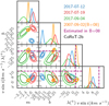 |
Fig. A.1 Posterior probability distributions for four free parameters (including the slope of out-of-transit) space of fit to individual RM observations of CoRoT-2b. |
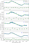 |
Fig. A.2 RM observations of CoRoT-2b during several nights. The green line displays the best fitted RM model (also considering the slope of out-of-transit as free parameter). The blue region shows the zone where 68% of the model solutions reside. In each panel the residuals are shown in the bottom panel. |
Appendix B Macro-turbulence as free parameter
In this section, we evaluate the consequence of leaving the macro-turbulence (Z) as an extra free parameter in our fitting procedure. Similar to Appendix A, we tested it on CoRoT-2b RM observations and repeated the fitting procedure on each individual RM observation. We considered a uniform (uninformative) prior on Z from 1 to 10 km s−1. We present the posterior probability distributions of all three free parameters in Fig. B.1. As our results show, the posterior distributions in vsini − λ parameter space is not affected by leaving macro-turbulence as a free parameter (cf. the posterior distribution of v sin i − λ in this figure with the posterior distribution of vsini − λ in Fig. 1). Therefore, our test shows that the impact of leaving macro-turbulence as a free parameter does not affect the estimated λ, which supports our choice.
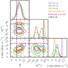 |
Fig. B.1 Posterior probability distributions of three free parameters (including macro-turbulence) space of fit to individual RM observations of CoRoT-2b. |
Appendix C Best fitted model to individual RM observations
In this section we present each individual RM observation (obtained during different nights) for each of our targets with their best fitted model, as obtained in Sect. 3. Moreover, we overplotted the best fitted model to the folded RM (dashed red line) to help the readers to visually identify the variation in the RM curves from transit to transit.
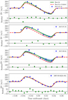 |
Fig. C.1 RMobservation of CoRoT-2b during several nights. The green line displays the best fitted RM model and the blue region shows the zone where 68% of the model solutions reside. In each panel the residuals are shown in the bottom panel. The red dashed lines show the best fitted RM model obtained from the folded RM observations from Fig. 4. |
Appendix D Radial velocities
In this section we present our targets’ RV measurements derived from the HARPS pipeline.
RV measurements of CoRoT-2 derived from the HARPS pipeline.
References
- Addison, B. C., Tinney, C. G., Wright, D. J., et al. 2013, ApJ, 774, L9 [NASA ADS] [CrossRef] [Google Scholar]
- Akinsanmi, B., Oshagh, M., Santos, N. C., & Barros, S. C. C. 2018, A&A, 609, A21 [NASA ADS] [CrossRef] [EDP Sciences] [Google Scholar]
- Albrecht, S., Winn, J. N., Johnson, J. A., et al. 2012, ApJ, 757, 18 [NASA ADS] [CrossRef] [Google Scholar]
- Barros, S. C. C., Boué, G., Gibson, N. P., et al. 2013, MNRAS, 430, 3032 [NASA ADS] [CrossRef] [Google Scholar]
- Baruteau, C., Crida, A., Paardekooper, S.-J., et al. 2014, Protostars and Planets VI (Tucson, AZ: University of Arizona Press), 667 [Google Scholar]
- Batygin, K. 2012, Nature, 491, 418 [NASA ADS] [CrossRef] [PubMed] [Google Scholar]
- Bayliss, D. D. R., Winn, J. N., Mardling, R. A., & Sackett, P. D. 2010, ApJ, 722, L224 [NASA ADS] [CrossRef] [Google Scholar]
- Bocquet, S., & Carter, F. W. 2016, J. Open Source Softw., 1 [Google Scholar]
- Bouchy, F., Queloz, D., Deleuil, M., et al. 2008, A&A, 482, L25 [NASA ADS] [CrossRef] [EDP Sciences] [Google Scholar]
- Boué, G., Oshagh, M., Montalto, M., & Santos, N. C. 2012, MNRAS, 422, L57 [NASA ADS] [Google Scholar]
- Bourrier, V., & Hébrard, G. 2014, A&A, 569, A65 [NASA ADS] [CrossRef] [EDP Sciences] [Google Scholar]
- Brown, D. J. A., Triaud, A. H. M. J., Doyle, A. P., et al. 2017, MNRAS, 464, 810 [NASA ADS] [CrossRef] [Google Scholar]
- Burdanov, A., Delrez, L., Gillon, M., et al. 2017, SPECULOOS Exoplanet Search and Its Prototype on TRAPPIST (Cham, Switzerland: Springer), 130 [Google Scholar]
- Cegla, H. M., Lovis, C., Bourrier, V., et al. 2016a, A&A, 588, A127 [NASA ADS] [CrossRef] [EDP Sciences] [Google Scholar]
- Cegla, H. M., Oshagh, M., Watson, C. A., et al. 2016b, ApJ, 819, 67 [NASA ADS] [CrossRef] [Google Scholar]
- Cosentino, R., Lovis, C., Pepe, F., et al. 2012, in Ground-based and Airborne Instrumentation for Astronomy IV, Proc. SPIE, 8446, 84461V [CrossRef] [Google Scholar]
- Crida, A., & Batygin, K. 2014, A&A, 567, A42 [NASA ADS] [CrossRef] [EDP Sciences] [Google Scholar]
- Czesla, S., Huber, K. F., Wolter, U., Schröter, S., & Schmitt, J. H. M. M. 2009, A&A, 505, 1277 [NASA ADS] [CrossRef] [EDP Sciences] [Google Scholar]
- Dai, F., Winn,J. N., Yu, L., & Albrecht, S. 2017, AJ, 153, 40 [NASA ADS] [CrossRef] [Google Scholar]
- Dawson, R. I., & Johnson, J. A. 2018, ARA&A, 56, 175 [NASA ADS] [CrossRef] [Google Scholar]
- de Mooij, E. J. W., Watson, C. A., & Kenworthy, M. A. 2017, MNRAS, 472, 2713 [NASA ADS] [CrossRef] [Google Scholar]
- Di Gloria, E., Snellen, I. A. G., & Albrecht, S. 2015, A&A, 580, A84 [NASA ADS] [CrossRef] [EDP Sciences] [Google Scholar]
- Esposito, M., Covino, E., Desidera, S., et al. 2017, A&A, 601, A53 [NASA ADS] [CrossRef] [EDP Sciences] [Google Scholar]
- Figueira, P., Faria, J. P., Adibekyan, V. Z., Oshagh, M., & Santos, N. C. 2016, Orig. Life Evol. Biosph., 46, 385 [NASA ADS] [CrossRef] [Google Scholar]
- Foreman-Mackey, D., Hogg, D. W., Lang, D., & Goodman, J. 2013, PASP, 125, 306 [CrossRef] [Google Scholar]
- Gillon, M. 2018, Nat. Astron., 2, 344 [NASA ADS] [CrossRef] [Google Scholar]
- Gillon, M., Anderson, D. R., Triaud, A. H. M. J., et al. 2009, A&A, 501, 785 [NASA ADS] [CrossRef] [EDP Sciences] [Google Scholar]
- Gillon, M., Jehin, E., Magain, P., et al. 2011, in Eur. Phys. J. Web Conf., 11, 06002 [Google Scholar]
- Hébrard, G., Bouchy, F., Pont, F., et al. 2008, A&A, 488, 763 [NASA ADS] [CrossRef] [EDP Sciences] [Google Scholar]
- Hébrard, G., Ehrenreich, D., Bouchy, F., et al. 2011, A&A, 527, L11 [NASA ADS] [CrossRef] [EDP Sciences] [Google Scholar]
- Hébrard, G., Collier Cameron, A., Brown, D. J. A., et al. 2013, A&A, 549, A134 [NASA ADS] [CrossRef] [EDP Sciences] [Google Scholar]
- Hellier, C., Anderson, D. R., Collier-Cameron, A., et al. 2011, ApJ, 730, L31 [NASA ADS] [CrossRef] [Google Scholar]
- Holt, J. R. 1893, Astronomy and Astro-physics (formerly The Sidereal Messenger), 12, 646 [NASA ADS] [Google Scholar]
- Ioannidis, P., Huber, K. F., & Schmitt, J. H. M. M. 2016, A&A, 585, A72 [NASA ADS] [CrossRef] [EDP Sciences] [Google Scholar]
- Jehin, E., Gillon, M., Queloz, D., et al. 2011, The Messenger, 145, 2 [NASA ADS] [Google Scholar]
- López-Morales, M., Triaud, A. H. M. J., Rodler, F., et al. 2014, ApJ, 792, L31 [NASA ADS] [CrossRef] [Google Scholar]
- Lovis, C., & Pepe, F. 2007, A&A, 468, 1115 [NASA ADS] [CrossRef] [EDP Sciences] [Google Scholar]
- Mancini, L., Southworth, J., Raia, G., et al. 2017, MNRAS, 465, 843 [NASA ADS] [CrossRef] [Google Scholar]
- Mayor, M., Pepe, F., Queloz, D., et al. 2003, The Messenger, 114, 20 [NASA ADS] [Google Scholar]
- McLaughlin, D. B. 1924, ApJ, 60, 22 [NASA ADS] [CrossRef] [Google Scholar]
- Močnik, T., Southworth, J., & Hellier, C. 2017, MNRAS, 471, 394 [NASA ADS] [CrossRef] [Google Scholar]
- Neveu-VanMalle, M., Queloz, D., Anderson, D. R., et al. 2016, A&A, 586, A93 [NASA ADS] [CrossRef] [EDP Sciences] [Google Scholar]
- Nutzman, P. A., Fabrycky, D. C., & Fortney, J. J. 2011, ApJ, 740, L10 [NASA ADS] [CrossRef] [Google Scholar]
- Ohta, Y., Taruya, A., & Suto, Y. 2009, ApJ, 690, 1 [NASA ADS] [CrossRef] [Google Scholar]
- Oshagh, M., Boué, G., Figueira, P., Santos, N. C., & Haghighipour, N. 2013a, A&A, 558, A65 [NASA ADS] [CrossRef] [EDP Sciences] [Google Scholar]
- Oshagh, M., Santos, N. C., Boisse, I., et al. 2013b, A&A, 556, A19 [NASA ADS] [CrossRef] [EDP Sciences] [Google Scholar]
- Oshagh, M., Santos, N. C., Boisse, I., et al. 2015a, in Eur. Phys. J. Web Conf., 101, 05003 [NASA ADS] [CrossRef] [EDP Sciences] [Google Scholar]
- Oshagh, M., Santos, N. C., Figueira, P., et al. 2015b, A&A, 583, L1 [NASA ADS] [CrossRef] [EDP Sciences] [Google Scholar]
- Oshagh, M., Dreizler, S., Santos, N. C., Figueira, P., & Reiners, A. 2016, A&A, 593, A25 [NASA ADS] [CrossRef] [EDP Sciences] [Google Scholar]
- Pepe, F., Mayor, M., Galland, F., et al. 2002, A&A, 388, 632 [NASA ADS] [CrossRef] [EDP Sciences] [Google Scholar]
- Pepe, F., Molaro, P., Cristiani, S., et al. 2014, Astron. Nachr., 335, 8 [NASA ADS] [CrossRef] [Google Scholar]
- Pollack, J. B., Hubickyj, O., Bodenheimer, P., et al. 1996, Icarus, 124, 62 [NASA ADS] [CrossRef] [Google Scholar]
- Quirrenbach, A., Amado, P. J., Caballero, J. A., et al. 2014, in Ground-based and Airborne Instrumentation for Astronomy V, Proc. SPIE, 9147, 91471F [Google Scholar]
- Rossiter, R. A. 1924, ApJ, 60, 15 [NASA ADS] [CrossRef] [Google Scholar]
- Sanchis-Ojeda, R., & Winn, J. N. 2011, ApJ, 743, 61 [NASA ADS] [CrossRef] [Google Scholar]
- Sanchis-Ojeda, R., Winn, J. N., Marcy, G. W., et al. 2013, ApJ, 775, 54 [NASA ADS] [CrossRef] [Google Scholar]
- Santerne, A., Hébrard, G., Deleuil, M., et al. 2014, A&A, 571, A37 [NASA ADS] [CrossRef] [EDP Sciences] [Google Scholar]
- Sedaghati, E., Boffin, H. M. J., Csizmadia, S., et al. 2015, A&A, 576, L11 [NASA ADS] [CrossRef] [EDP Sciences] [Google Scholar]
- Shporer, A., & Brown, T. 2011, ApJ, 733, 30 [NASA ADS] [CrossRef] [Google Scholar]
- Southworth, J., Tregloan-Reed, J., Andersen, M. I., et al. 2016, MNRAS, 457, 4205 [NASA ADS] [CrossRef] [Google Scholar]
- Stetson, P. B. 1987, PASP, 99, 191 [NASA ADS] [CrossRef] [Google Scholar]
- Tregloan-Reed, J., Southworth, J., & Tappert, C. 2013, MNRAS, 428, 3671 [NASA ADS] [CrossRef] [Google Scholar]
- Tregloan-Reed, J., Southworth, J., Burgdorf, M., et al. 2015, MNRAS, 450, 1760 [NASA ADS] [CrossRef] [Google Scholar]
- Triaud, A. H. M. J. 2017, The Rossiter-McLaughlin Effect in Exoplanet Research (Berlin: Springer), 2 [Google Scholar]
- Triaud, A. H. M. J., Collier Cameron, A., Queloz, D., et al. 2010, A&A, 524, A25 [NASA ADS] [CrossRef] [EDP Sciences] [Google Scholar]
- Winn, J. N., Noyes, R. W., Holman, M. J., et al. 2005, ApJ, 631, 1215 [NASA ADS] [CrossRef] [Google Scholar]
There could be reasons other than stellar activity that produce these variations, which we will discuss in Sect. 7.

Spectrographs lose photons due to slit losses, stray light, and scattered light. Moreover, spectrographs disperse photons over the detector where each pixel has a different readout noise. Therefore, spectrograph by construction required many more photons to reach the same S/N as photometric observations.
All Tables
Standard deviation of the residual between SOAP3.0 predicted RM and observed RM for models that ignore the spot crossing events and for models that take into account spot crossing events.
All Figures
|
Fig. 1 Posterior probability distributions in vsini − λ parameter space of all our targets obtained from the fit to individual RM observations obtained at different transits and on different nights. Each panel shows different planetary system, and in each panel different colors correspond to the different nights on which the RM observation were performed. The purple dashed line displays the reported value in the literature. B+08: Bouchy et al. (2008), H+11: Hellier et al. (2011), N+16: Neveu-VanMalle et al. (2016), G+09: Gillon et al. (2009), H+13: Hébrard et al. (2013), E+17: Esposito et al. (2017). |
| In the text | |
|
Fig. 2 Top panel: correlations between Δλ and log |
| In the text | |
|
Fig. 3 Posterior probability distributions in vsini − λ parameter space of all our targets obtained from the fit to the folded RM observations. Each panel shows different planetary system. The black dashed line displays median values of the posterior distributions, and the 1σ uncertainties taken to be the value enclosed in the 68.3% of the posterior distributions are shown with the black dotted line. |
| In the text | |
|
Fig. 4 Folded RM observations of our targets during several nights. The green line shows the best fitted RM model and blue region shows the zone where 68% of the model solutions reside. In each panel the residuals are shown in the bottom panel. |
| In the text | |
|
Fig. 5 Simultaneous photometric transit and RM observation of CoRoT-2b on the night of 12 July 2017 (top panels) and on night thenight of 19 July 2017 (bottom panels). The dark blue square represents the binned TRAPPIST photometric observations, and the dark blue filled circle the HARPS RM observation. The red line is the SOAP3.0 model without considering any stellar active regions. The green lines are the SOAP3.0 best fitted model to transit light curve taking into accountthree spots. |
| In the text | |
|
Fig. 6 Simultaneous photometric transits and RM observations of WASP-19b on the night of 5 May 2017 (top panels) and on the night of 9 May 2017 (bottom panels). The lines and points are the same as in Fig. 5. |
| In the text | |
|
Fig. 7 Simultaneous photometric transits and RM observations of Qatar-2b on the night of 10 July 2017. The photometric observationswere obtained from simultaneous observations of TRAPPIST and SPECULOOS. The lines and points are the same as in Fig. 5. |
| In the text | |
|
Fig. A.1 Posterior probability distributions for four free parameters (including the slope of out-of-transit) space of fit to individual RM observations of CoRoT-2b. |
| In the text | |
|
Fig. A.2 RM observations of CoRoT-2b during several nights. The green line displays the best fitted RM model (also considering the slope of out-of-transit as free parameter). The blue region shows the zone where 68% of the model solutions reside. In each panel the residuals are shown in the bottom panel. |
| In the text | |
|
Fig. B.1 Posterior probability distributions of three free parameters (including macro-turbulence) space of fit to individual RM observations of CoRoT-2b. |
| In the text | |
|
Fig. C.1 RMobservation of CoRoT-2b during several nights. The green line displays the best fitted RM model and the blue region shows the zone where 68% of the model solutions reside. In each panel the residuals are shown in the bottom panel. The red dashed lines show the best fitted RM model obtained from the folded RM observations from Fig. 4. |
| In the text | |
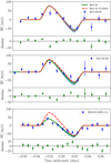 |
Fig. C.2 As for Fig. C.1, but for WASP-19b. |
| In the text | |
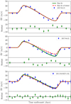 |
Fig. C.3 As for Fig. C.1, but for WASP-41b. |
| In the text | |
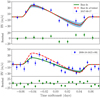 |
Fig. C.4 As for Fig. C.1, but for WASP-6b. |
| In the text | |
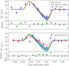 |
Fig. C.5 As for Fig. C.1, but for WASP-52b. |
| In the text | |
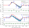 |
Fig. C.6 As for Fig. C.1, but for Qatar-2b. |
| In the text | |
Current usage metrics show cumulative count of Article Views (full-text article views including HTML views, PDF and ePub downloads, according to the available data) and Abstracts Views on Vision4Press platform.
Data correspond to usage on the plateform after 2015. The current usage metrics is available 48-96 hours after online publication and is updated daily on week days.
Initial download of the metrics may take a while.