| Issue |
A&A
Volume 619, November 2018
|
|
|---|---|---|
| Article Number | A9 | |
| Number of page(s) | 37 | |
| Section | Astronomical instrumentation | |
| DOI | https://doi.org/10.1051/0004-6361/201833620 | |
| Published online | 06 November 2018 | |
SPHERE/ZIMPOL high resolution polarimetric imager
I. System overview, PSF parameters, coronagraphy, and polarimetry⋆
1 ETH Zurich, Institute for Particle Physics and Astrophysics, Wolfgang-Pauli-Strasse 27, 8093 Zurich, Switzerland
e-mail: This email address is being protected from spambots. You need JavaScript enabled to view it.
2 NOVA Optical Infrared Instrumentation Group at ASTRON, Oude Hoogeveensedijk 4, 7991 PD Dwingeloo, The Netherlands
3 Université Grenoble Alpes, IPAG, 38000 Grenoble, France
4 CNRS, IPAG, 38000
Grenoble, France
5 European Southern Observatory, Alonso de Cordova 3107, Casilla 19001 Vitacura, Santiago 19, Chile
6 Istituto Ricerche Solari Locarno, Via Patocchi 57, 6605 Locarno Monti, Switzerland
7 Kiepenheuer-Institut für Sonnenphysik, Schneckstr. 6, 79104 Freiburg, Germany
8 Anton Pannekoek Astronomical Institute, University of Amsterdam, PO Box 94249 1090 GE Amsterdam, The Netherlands
9 LESIA, CNRS, Observatoire de Paris, Université Paris Diderot, UPMC, 5 place J. Janssen, 92190 Meudon, France
10 Leiden Observatory, Leiden University, PO Box 9513 2300 RA Leiden, The Netherlands
11 Laboratoire Lagrange, UMR7293, Université de Nice Sophia-Antipolis, CNRS, Observatoire de la Côte d’Azur, Boulevard de l’Observatoire, 06304 Nice, Cedex 4, France
12 INAF – Osservatorio Astronomico di Roma, via Frascati 33, 00087 Monte Porzio Catone, Italy
13 Max-Planck-Institut für Astronomie, Königstuhl 17, 69117 Heidelberg, Germany
14 INAF – Osservatorio Astronomico di Padova, Vicolo dell’Osservatorio 5, 35122 Padova, Italy
15 Aix Marseille Université, CNRS, CNES, LAM (Laboratoire d’Astrophysique de Marseille) UMR 7326, 13388 Marseille, France
16 Unidad Mixta International Franco-Chilena de Astronomia, CNRS/INSU UMI 3386 and Departemento de Astronomia, Universidad de Chile, Casilla 36-D, Santiago, Chile
17
European Southern Observatory, Karl Schwarzschild St, 2, 85748 Garching, Germany
18 ONERA, The French Aerospace Lab BP72, 29 avenue de la Division Leclerc, 92322 Châtillon Cedex, France
19 Centre de Recherche Astrophysique de Lyon, CNRS/ENSL Université Lyon 1, 9 av. Ch. André, 69561 Saint-Genis-Laval, France
20 INAF – Osservatorio Astrofisico di Arcetri, Largo E. Fermi 5, 50125 Firenze, Italy
21 Geneva Observatory, University of Geneva, Chemin des Mailettes 51, 1290 Versoix, Switzerland
Received:
12
July
2018
Accepted:
3
August
2018
Abstract
Context. The SPHERE “planet finder” is an extreme adaptive optics (AO) instrument for high resolution and high contrast observations at the Very Large Telescope (VLT). We describe the Zurich Imaging Polarimeter (ZIMPOL), the visual focal plane subsystem of SPHERE, which pushes the limits of current AO systems to shorter wavelengths, higher spatial resolution, and much improved polarimetric performance.
Aims. We present a detailed characterization of SPHERE/ZIMPOL which should be useful for an optimal planning of observations and for improving the data reduction and calibration. We aim to provide new benchmarks for the performance of high contrast instruments, in particular for polarimetric differential imaging.
Methods. We have analyzed SPHERE/ZIMPOL point spread functions (PSFs) and measure the normalized peak surface brightness, the encircled energy, and the full width half maximum (FWHM) for different wavelengths, atmospheric conditions, star brightness, and instrument modes. Coronagraphic images are described and the peak flux attenuation and the off-axis flux transmission are determined. Simultaneous images of the coronagraphic focal plane and the pupil plane are analyzed and the suppression of the diffraction rings by the pupil stop is investigated. We compared the performance at small separation for different coronagraphs with tests for the binary α Hyi with a separation of 92 mas and a contrast of Δm ≈ 6m. For the polarimetric mode we made the instrument calibrations using zero polarization and high polarization standard stars and here we give a recipe for the absolute calibration of polarimetric data. The data show small (< 1 mas) but disturbing differential polarimetric beam shifts, which can be explained as Goos-Hähnchen shifts from the inclined mirrors, and we discuss how to correct this effect. The polarimetric sensitivity is investigated with non-coronagraphic and deep, coronagraphic observations of the dust scattering around the symbiotic Mira variable R Aqr.
Results. SPHERE/ZIMPOL reaches routinely an angular resolution (FWHM) of 22−28 mas, and a normalized peak surface brightness of SB0 − mstar ≈ −6.5m arcsec−2 for the V-, R- and I-band. The AO performance is worse for mediocre ≳1.0″ seeing conditions, faint stars mR ≳ 9m, or in the presence of the “low wind” effect (telescope seeing). The coronagraphs are effective in attenuating the PSF peak by factors of > 100, and the suppression of the diffracted light improves the contrast performance by a factor of approximately two in the separation range 0.06″−0.20″. The polarimetric sensitivity is Δp < 0.01% and the polarization zero point can be calibrated to better than Δp ≈ 0.1%. The contrast limits for differential polarimetric imaging for the 400 s I-band data of R Aqr at a separation of ρ = 0.86″ are for the surface brightness contrast SBpol( ρ)−mstar ≈ 8m arcsec−2 and for the point source contrast mpol( ρ)−mstar ≈ 15m and much lower limits are achievable with deeper observations.
Conclusions. SPHERE/ZIMPOL achieves imaging performances in the visual range with unprecedented characteristics, in particular very high spatial resolution and very high polarimetric contrast. This instrument opens up many new research opportunities for the detailed investigation of circumstellar dust, in scattered and therefore polarized light, for the investigation of faint companions, and for the mapping of circumstellar Hα emission.
Key words: instrumentation: adaptive optics / instrumentation: high angular resolution / instrumentation: polarimeters / instrumentation: detectors / planetary systems / circumstellar matter
Based on observations collected at La Silla and Paranal Observatory, ESO (Chile), Program ID: 60.A-9249 and 60.A-9255.
© ESO 2018
1. Introduction
The SPHERE “planet finder” instrument has been successfully installed and commissioned in 2014 at the VLT. The main task of this instrument is the search and investigation of extra-solar planets around bright stars mR ≲ 10m. Therefore SPHERE is optimized for high contrast and diffraction limited resolution observation in the near-IR and the visual spectral region using an extreme adaptive optics (AO) system, stellar coronagraphs, and three focal plane instruments for differential imaging. General technical descriptions of the instrument are given in Beuzit et al. (2008), Kasper et al. (2012), and the SPHERE user manual and related technical websites1 of the European Southern Observatory (ESO). SPHERE is a very powerful facility instrument which provides a broad suite of sophisticated instrument modes for the very demanding investigation of extra-solar planetary systems. Essentially all of these modes also provide unique observing opportunities for the study of the immediate circumstellar environment of bright stars. Technical results about the on-sky performance of the SPHERE instrument are given in Dohlen et al. (2016), and on-sky results for the AO-system are described in Fusco et al. (2016) and Milli et al. (2017). A series of first SPHERE science papers demonstrates the performance of various observing modes of this instrument (e.g. Vigan et al. 2016; Maire et al. 2016a; Zurlo et al. 2016; Bonnefoy et al. 2016). However, the SPHERE instrument is complex and therefore it is appropriate to give more specific descriptions on individual subsystems and this is the first of a few technical papers for the visual focal plane instrument ZIMPOL.
ZIMPOL, the Zurich Imaging Polarimeter, works in the spectral range from 500 nm to 900 nm and provides, thanks to the SPHERE AO system and visual coronagraph, high resolution (≈20–30 mas) and high contrast imaging and imaging polarimetry for the immediate surroundings (ρ < 4 arcsec) of bright stars. SPHERE/ZIMPOL includes a very innovative concept for high performance imaging polarimetry using a fast modulation – demodulation technique and it is tuned for very high contrast polarimetry of reflected light from planetary system. Beside this it can also be used as a high contrast imager offering angular differential imaging and simultaneous spectral differential imaging.
Previous publications on ZIMPOL describe the science goal (Schmid et al. 2006a), the expected performance (Thalmann et al. 2008), and give reports about the concept of ZIMPOL (Gisler et al. 2004; Joos 2007; de Juan Ovelar et al. 2012), the instrument design and component tests (Roelfsema et al. 2010, 2011; Pragt et al. 2012; Bazzon et al. 2012; Schmid et al. 2012) and system testing (Roelfsema et al. 2014, 2016). Some early science results based on SPHERE/ZIMPOL observations are given in Thalmann et al. (2015), Garufi et al. (2016), Kervella et al. (2016), Stolker et al. (2016), Khouri et al. (2016), Avenhaus et al. (2017), Ohnaka et al. (2017a) and Engler et al. (2017). Schmid et al. (2017) also gives technical information about Hα imaging and the flux calibration of ZIMPOL data.
Previous publications on ZIMPOL describe the science goal (Schmid et al. 2006a), the expected performance (Thalmann et al. 2008), and give reports about the concept of ZIMPOL (Gisler et al. 2004; Joos 2007; de Juan Ovelar et al. 2012), the instrument design and component tests (Roelfsema et al. 2010, 2011; Pragt et al. 2012; Bazzon et al. 2012; Schmid et al. 2012) and system testing (Roelfsema et al. 2014, 2016). Some early science results based on SPHERE/ZIMPOL observations are given in Thalmann et al. (2015), Garufi et al. (2016), Kervella et al. (2016), Stolker et al. (2016), Khouri et al. (2016), Avenhaus et al. (2017), Ohnaka et al. (2017a) and Engler et al. (2017). Schmid et al. (2017) also gives technical information about Hα imaging and the flux calibration of ZIMPOL data.
Previous publications on ZIMPOL describe the science goal (Schmid et al. 2006a), the expected performance (Thalmann et al. 2008), and give reports about the concept of ZIMPOL (Gisler et al. 2004; Joos 2007; de Juan Ovelar et al. 2012), the instrument design and component tests (Roelfsema et al. 2010, 2011; Pragt et al. 2012; Bazzon et al. 2012; Schmid et al. 2012) and system testing (Roelfsema et al. 2014, 2016). Some early science results based on SPHERE/ZIMPOL observations are given in Thalmann et al. (2015), Garufi et al. (2016), Kervella et al. (2016), Stolker et al. (2016), Khouri et al. (2016), Avenhaus et al. (2017), Ohnaka et al. (2017a) and Engler et al. (2017). Schmid et al. (2017) also gives technical information about Hα imaging and the flux calibration of ZIMPOL data.
Previous publications on ZIMPOL describe the science goal (Schmid et al. 2006a), the expected performance (Thalmann et al. 2008), and give reports about the concept of ZIMPOL (Gisler et al. 2004; Joos 2007; de Juan Ovelar et al. 2012), the instrument design and component tests (Roelfsema et al. 2010, 2011; Pragt et al. 2012; Bazzon et al. 2012; Schmid et al. 2012) and system testing (Roelfsema et al. 2014, 2016). Some early science results based on SPHERE/ZIMPOL observations are given in Thalmann et al. (2015), Garufi et al. (2016), Kervella et al. (2016), Stolker et al. (2016), Khouri et al. (2016), Avenhaus et al. (2017), Ohnaka et al. (2017a) and Engler et al. (2017). Schmid et al. (2017) also gives technical information about Hα imaging and the flux calibration of ZIMPOL data.
Many technical aspects must be considered for carrying out well optimized observations and calibrations with an instrument like ZIMPOL, which combines diffraction-limited imaging using extreme adaptive optics, coronagraphy, and differential techniques like polarimetry, or angular and spectral differential imaging. It is not possible to cover all these topics in detail in one paper and therefore we focus on a basic technical description and on aspects which are special to SPHERE/ZIMPOL when compared to other high contrast instruments. This should serve as a starting point for potential SPHERE/ZIMPOL users to carry out well optimized observations and data analyzes for exploiting the full potential of this instrument. We plan that subsequent papers will address other aspects of SPHERE/ZIMPOL, such as astrometry, precision photometry, a detailed technical assessment of the high performance polarimetry mode and more.
This paper is organized as follows. The next section gives a brief overview on the SPHERE common path and a detailed description of the ZIMPOL subsystem, imaging properties, the ZIMPOL polarimetry, the detectors and detector calibrations, and the filters. Section 3 characterizes the “typical” point spread functions (PSFs) and describes special cases, like faint stars, poor atmospheric conditions, or particular instrumental effects. The topic of Sect. 4 is the SPHERE visual coronagraph and the comparison of coronagraphic test measurements taken with different focal plane masks. SPHERE/ZIMPOL polarimetry is described in detail in Sect. 5 including the concept for the control of the polarimetric signal and the correction of the measurements based on calibrations of the telescope, the instrument, and the detectors. Further we discuss the polarimetric differential beamshift, a disturbing effect which is new for astronomical optics and which was not anticipated in the design of this instrument. Then, we illustrate the very good polarimetric performance of ZIMPOL with test observations of the system R Aqr. We conclude in Sect. 6 with a summary of the most outstanding technical properties of SPHERE/ZIMPOL and an outline of the new research opportunities offered by this instrument.
2. The visual channel of SPHERE
The SPHERE visual channel covers the wavelength range from 500 to 900 nm and provides observational modes for imaging, spectral differential imaging, angular differential imaging and polarimetric differential imaging. The next subsection gives a brief overview of the SPHERE common path while the visual focal plane instrument ZIMPOL is described in detail in the following subsections.
2.1. Common path and infrastructure – CPI
Figure 1 gives a simplified block diagram of those parts of the SPHERE main bench or “common path and infrastructure” (CPI) system which are relevant for visual observations. Table 1 lists the components along the beam indicating the rotating, insertable, and exchangeable components and those which are only in the beam for polarimetry (see also the colors in Fig. 1).
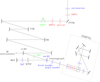 |
Fig. 1. Block diagram of the SPHERE common path (CPI) up to the beam splitter vi.BS and the SPHERE visual channel. The blue color indicates exchangeable components, green are rotating components, and red components are only inserted for polarimetry. The ZIMPOL box is shown in detail in Fig. 2. |
Optical components of the VLT and SPHERE CPI visual path.
The heart of the SPHERE instrument is the extreme adaptive optics (AO) system, which corrects for the variable wave-front distortions introduced by the rapidly changing Earth’s atmosphere. At the same time the AO corrects also for aberrations introduced by the telescope and the SPHERE instrument (Fusco et al. 2014; Sauvage et al. 2016b). The AO system needs a bright natural guide star in the center of the science field as wave front probe, preferentially with a brightness mR ≲ 10m. The AO performance depends strongly on the atmospheric conditions and the guide star brightness (Sauvage et al. 2016b) as described in Sect. 3. Essential components of the AO system are the Shack-Hartmann wave front sensor (WFS), which measures the wave front distortions, the fast high-order deformable mirror (DM), the fast tip-tilt mirror (TTM), and the pupil tip-tilt mirror (PTTM) which correct for the measured distortions.
The CPI includes in addition an image derotator (DROT) which can be used in three different rotation modes: (i) to stabilize the sky image on the detector, (ii) to fix the orientation of the telescope pupil, or (iii) to keep the instrument polarization stabilized. The visual-infrared beam splitter (vi.BS) transmits long wavelengths λ > 950 nm to the IR science channel and reflects the short wavelengths λ < 950 nm to the wave front sensor arm and ZIMPOL. The IR channel includes the IR-coronagraph (Boccaletti et al. 2008) and two focal plane instruments, the infrared double beam imager and spectrograph IRDIS (Dohlen et al. 2008; Vigan et al. 2014) and the integral field spectrograph IFS (Claudi et al. 2008).
The visual beam is further split after the visual atmospheric dispersion corrector (ADC) by one of two exchangeable beam splitters (zw.BS) which reflect part of the light to the wave front sensor arm and transmits the other part to the visual coronagraph and ZIMPOL. There is a gray beam-splitter transmitting about 79% of the light to ZIMPOL and 21% to the WFS, and a dichroic beam-splitter transmitting the wavelengths 600−680 nm to ZIMPOL and reflecting the other wavelengths within the 500−950 nm range, or about 80% of the light depending on the color of the central star, to the WFS.
The wave front sensor arm includes a tip-tilt plate (WTTP) for the fine centering of the central AO guide star on a coronagraphic focal plane mask, or another position in the field of view within about 0.6″ from the optical axis. In front of the WFS one can also select between a large, medium or small field mask as spatial filter to optimize the AO performance (Fusco et al. 2016).
Furthermore, the CPI includes two insertable and rotatable half-wave plates (HWP1 and HWP2) and polarimetric calibration components (pol.cal) for polarimetric imaging with ZIMPOL as will be described later in Sect. 5.2.
Different calibration light sources and components can be inserted inside SPHERE at the VLT-Nasmyth focus (Wildi et al. 2009, 2010). For the visual science channel there is a flat field source with a continuous spectrum for detector flat-fielding. This source can be combined with a mask with a grid of holes for measurements of the SPHERE/ZIMPOL image scale and distortions. In addition, there is a point source with a continuous spectrum for measurements and checks of the instrument alignment. The brightness of the sources can be adjusted with neutral density filters also located in the calibration unit.
2.2. The Zurich imaging polarimeter
A block diagram for the Zurich IMaging POLarimeter (ZIMPOL) is shown in Fig. 2 and a list of all components is given in Table 2. ZIMPOL is a two arm imager with a polarization beam splitter (BS). The ZIMPOL common path consists of a collimated beam section with an intermediate pupil just before ZIMPOL, at the position of the coronagraphic pupil mask wheel. This pupil has a diameter of 6 mm and it defines the interface between CPI and ZIMPOL. Polarimetric components can be inserted and removed in the ZIMPOL common path without changing the image focus. The following subsections describe the imaging properties of this setup, the ZIMPOL polarimetric principle, the polarimetric components, the special detector properties, and the ZIMPOL filters. Previous publications on ZIMPOL give more information about the opto-mechanical design (Roelfsema et al. 2010), optical alignment procedures (Pragt et al. 2012), test results at various phases of the project (Roelfsema et al. 2011, 2014, 2016), the detectors (Schmid et al. 2012), and the polarimetric calibration concept (Bazzon et al. 2012).
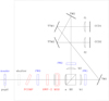 |
Fig. 2. Block diagram for ZIMPOL with exchangeable components plotted in blue, while red components are only inserted for polarimetry. |
List of all components in ZIMPOL.
2.2.1. ZIMPOL imaging properties
The ZIMPOL subsystem is optimized for polarimetric imaging but provides at the same time also very good imaging capabilities. In this section we describe the imaging properties of ZIMPOL, which apply for imaging and polarimetric imaging. For polarimetry, additional components are inserted in CPI and ZIMPOL and different detector modes are used, which reduce the overall instrument throughput by about a factor 0.85 with respect to non-polarimetric imaging.
For imaging the three red polarimetric components in the ZIMPOL block diagram (Fig. 2) are removed from the beam and there remains only the shutter and filter wheel FW0 in the common path. The polarization beam splitter creates then the two camera arms 1 and 2, each equipped with its own filter wheel FW1 or FW2, own detectors CCD1 or CCD2, own imaging optics (lenses b1,f1 or b2,f2), and own movable folding mirrors TM1,TTM1 or TM2,TTM2 for dithering and the selection of the detector field of view.
The beam-splitter includes on the entrance side lens “a”, a first common component of the camera optics. It is glued onto the beam splitter in order to avoid back-reflections (and ghost images) from the surfaces of the beam-splitter. Lens “a” produces together with “b1” or “b2” the converging beams with an f-ratio of 221 producing an image scale of 0.12 arcsec/mm or a pixel scale of about 3.6 mas pix−1 on the CCD detectors. The detectors have an active area of about 3.0 × 3.0 cm2 or about 1000 × 1000 pixels covering a detector field of view of about 3.6″×3.6″. There are optical image distortions and the dominant effect is an anamorphism which originates from the SPHERE common path optics located after the image derotator. This stretches for ZIMPOL the image scale expressed as mas pix−1 by a factor of about 1.006 in the detector row or x-direction, which is perpendicular to the CCD charge shifting direction. In field stabilized observations without field angle offset a square pixel covers an area, which is slightly elongated in east-west direction when projected onto the sky, like for the IRDIS and IFS near-IR instruments (see also Maire et al. 2016b). Detailed measurements of these distortions and the derivation of an accurate astrometric calibration for ZIMPOL will be described in Paper II (Ginski et al., in prep.).
ZIMPOL allows imaging in two channels using either a filter in the common path wheel FW0, or combining filters from the wheels FW1 in arm 1 and FW2 in arm 2 (see Sect. 2.4). Differential spectral imaging can be achieved by using different filters in FW1 and FW2. The filters in FW1 and FW2 can be combined with a neutral density filter located in FW0 in order to avoid detector saturation of bright sources.
Off-axis fields. The SPHERE/ZIMPOL optical field of view has a diameter of 8″ (6.67 cm) and is about four times larger than the detector field of view. This 8″-field is defined by the wide field “WF” focal plane masks in the coronagraph. To access the whole field of view offered by SPHERE/ZIMPOL, it is possible to move the image on the detector with the tip-tilt mirrors TTM1 or TTM2 and tip mirrors TM1 or TM2 in the two arms. Field lenses f1 or f2 and tip-mirrors are required to achieve, also for off-axis fields, a perpendicular illumination of the cylindrical micro-lenses and stripe masks in front of the special ZIMPOL detectors (see Sect. 2.3). To simplify the operation of ZIMPOL the instrument software allows only identical dithering and field offsets in arm 1 and arm 2. Optimized mirror settings have been pre-defined and tested for observations of the field center and eight off-axis fields (OAF1 – OAF8). The selectable off-axis fields are shown in Fig. 3 and approximate values for the offsets are given in Table 3. The off-axis fields avoid the central star and the surrounding ρ ≲ 0.8″ strong light halo. This enables long exposures with broad-band filters in the off-axis fields without saturation by light from the typically much brighter central star.
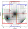 |
Fig. 3. Full ZIMPOL instrument field for the astrometric field 47 Tuc. The central detector field is plotted in black, while colors are used for the 8 pre-defined off-axis fields OAF1-OAF8. The off-axis fields have been shifted slightly (red to the left, blue to the right, and green up) for better visibility. No data are available for OAF4 because of an observational error. |
Approximate offsets for the centers of the off-axis fields (OAF).
The sky region shown in Fig. 3 is the SPHERE astrometric reference field 47 Tuc = NGC 104 (Maire et al. 2016b). This field is centered on the bright asymptotic giant branch (AGB) star 2MASS J00235767 − 7205296, which is also star “MMS12” in the mid-IR study of Momany et al. (2012). Also “MMS36”, the southern star of the pair in the SE and the star “MMS11” (also 2MASS J00235692 − 7205325) just outside the field in the SW are bright AGB stars. The northern star of the SE pair is the well studied post-AGB star Cl* NGC 104 BS (BS for bright star) with spectral type B8 III, the brightest star in 47 Tuc in the V-band V = 10.7m and even more prominent in the near and far UV (e.g. Dixon et al. 1995; Schiavon et al. 2012). The catalog of McLaughlin et al. (2006) and a study of Bellini (priv. commun., see also Bellini et al. 2014) provide accurate HST astrometry of most stars visible in Fig. 3 and they can be used for the astrometric calibrations for the central field, but also the off-axis fields of ZIMPOL.
The ZIMPOL image rotation modes. The SPHERE bench is fixed to the VLT Nasmyth platform A of UT3 and the sky image rotates in the telescope focus (“tf”) or the entrance focus of the instrument like
 (1)
(1)
where θpara is the parallactic angle and a the telescope altitude. The field orientation on the detector is defined by the image rotation introduced by DROT.
For the ZIMPOL imaging mode one can choose between field stabilized and pupil stabilized observations. In the first case the sky image is fixed and NCCD, the north direction on the CCD-detector after applying image flips in the data preprocessing, is given by
 (2)
(2)
where the angle NCCD is measured from the vertical or y-direction in counter-clockwise direction. There is a small rotational offset θ0 ≈ 2°, which is not exactly identical for CCD1 and CCD2, and which can be accurately determined with astrometric calibrations (Ginsky et al., in prep.). The term δθ stands for the user defined field orientation angle offset (see Fig. 22).
In pupil stabilized mode the telescope pupil is stabilized on the detector and the field rotates in step with the parallactic angle. This may introduce image smearing for long integrations, if the rotation during tDIT is too large.
For polarimetric imaging one can choose between static derotator mode, called P1, and field stabilized mode P2. In P1 mode the derotator is fixed and the field rotates on the CCD as
 (3)
(3)
but also the telescope pupil moves with a(t). The advantage of this mode is an accurate calibration of the telescope polarization, because derotator and all following components (except for the atmospheric dispersion corrector) are in a fixed orientation. The rotation law for P2 is identical to the field stabilized mode in imaging.
2.2.2. The ZIMPOL principle
Strong, variable speckles from the bright star are the main problem for high contrast imaging from the ground. ZIMPOL is optimized for high precision imaging polarimetry under such conditions because the speckle noise can be strongly reduced with an imaging polarimeter based on a fast modulation-demodulation technique. A polarization modulator and a polarizer (or a polarization beam splitter) convert the fractional polarization signal into a fractional modulation of the intensity signal, which is then measured by a masked, demodulating imaging detector as shown schematically in Fig. 4.
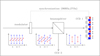 |
Fig. 4. ZIMPOL principle: The modulator switches in one cycle n the polarization direction between I⊥ and I∥. The polarization beam splitter selects for each channel only one polarization mode so that a polarization signal is converted into an intensity modulation. The masked CCDs demodulate the signal with charge-shifting, which is synchronized with the modulator. |
A polarimetric modulation with a frequency of about 1 kHz is sufficient to “freeze” the speckle variations introduced by the atmospheric turbulence in the differential polarimetric measurement. This requirement is realized in SPHERE/ZIMPOL with a modulation using a ferro-electric liquid crystal (FLC) retarder and CCD array detectors for the demodulation. On the CCD “every second row” is masked so that photo-charges created in the open rows during one half of the modulation cycle are shifted for the second half of the cycle to the next masked row, which is used as temporary buffer. The charge shifting is synchronized with the modulator switching, so that two images, the “even-row” and the “odd-row” subframes, with opposite linear polarization modes I⊥ and I∥ are built up. Photo-electrons can be collected during hundreds or thousands of modulation cycles before the detector is read out. The difference of the two images is proportional to the polarization flux and the sum proportional to the intensity
 (4)
(4)
Important advantages of the ZIMPOL technique are:
-
the images for opposite polarization states are created essentially simultaneously because the modulation is faster than the speckle variations and instrument drifts,
-
allows a fast modulation without high frame rates so that the read-out noise is low,
-
both images are recorded with the same pixels, reducing significantly flatfielding requirements and alignment issues for the difference image,
-
differential aberrations between the two images with opposite polarization are very small.
ZIMPOL is a single beam technique which could also be used with a polarizer, but then 50% of the light is lost. With a polarization beam splitter all light is used and the same polarimetric information is encoded in both channels. The two channels can be combined but they can also be used as separate but simultaneous measurements, for example by using different filters in the two arms.
2.2.3. ZIMPOL polarimetric setup
This section describes the properties of the polarimetric components in ZIMPOL while Sect. 5.2 explains how they are used to obtain well calibrated polarization data. ZIMPOL has three polarimetric components, the ferro-electric liquid crystal (FLC) modulator assembly, the polarization compensator (PCOMP) and a half-wave plate (HWPZ) which are only inserted for polarimetric observations (indicated in red in Fig. 2). Further polarimetric components are the polarization beam splitter and the polarimetric calibration components in FW0. The other key elements for polarimetry are the demodulating CCD detectors described in the next section.
PCOMP and HWPZ. The polarization compensator plate (PCOMP) is required to reduce the instrument polarization of about 2−3% introduced by the DROT (derotator) mirrors in CPI. A low instrument polarization is important for a good charge trap compensation and for reducing the impact of non-linearity of the detectors on the achievable polarization sensitivity. PCOMP is an uncoated, inclined glass plate (fused silica n = 1.45–1.46), where the two surfaces deflect more I⊥ than I∥ so that a linear polarization of the incoming beam  can be reduced for the transmitted beam pt = pi − Δp, if the inclined plate has a perpendicular orientation θPCOMP = θpol + 90°. The polarimetric compensation depends on the inclination angle of the plate, according to the Fresnel formulae (e.g. Born & Wolf 1999; Collett 1992). The PCOMP orientation rotates in step with DROT and the inclination can be adjusted. In the commissioning a good compensation for the entire wavelength range and all DROT orientations was found for iPCOMP = 25°. For this angle the two surfaces deflect together about
  and
and  . For small polarization pi < 5% the total transmission is It ≈ 0.93Ii and the polarization in the transmitted beam is reduced according to pt ≈ pi − 2.0%
ZIMPOL has two DROT-modes for polarimetry, P1-mode with fixed DROT and a rotating sky field on the detector, and P2-mode with rotating DROT and fixed field on the detector. In P1-mode, DROT and PCOMP are both fixed and in P2 they rotate synchronously. In P2-mode an additional achromatic half-wave plate (HWPZ) must be introduced, to rotate the polarization to be measured, which passes the DROT as I⊥ and I∥, into the I⊥ and I∥ orientation of the polarimeter. For this, also HWPZ must be on a rotational stage and its orientation is θHWPZ = θDROT/2.
ZIMPOL measures the linear polarization PZ = I⊥ − I∥ perpendicular and parallel to the SPHERE bench only. HWP2 and DROT in the common path and HWPZ within ZIMPOL are responsible for the correct rotation of the sky polarization into the ZIMPOL system. The achromatic half-wave plates are made of quartz and MgF2 retarders in optical contact2.
The FLC modulator. The ferro-electric liquid crystal (FLC) polarization modulator is a key component in ZIMPOL. An FLC retarder is a zero order half wave plate where the orientation of the optical axis can be switched by about 45° by changing the sign of the applied voltage through the FLC layer. A fast switch time in the range of 50 μs is required to achieve a good efficiency for a modulation cycle frequency on the order 1 kHz. The selected FLC retarder achieves this fast switching only when the operation temperature is in the range 20°−30° Celsius. Also the switching angle depends slightly on temperature (Gandorfer 1999; Gisler et al. 2003). Because the FLC retarder has to be warmer than the rest of the SPHERE instrument (0 ° −15°C) it is thermally insulated in a vacuum housing to avoid air turbulence in the instrument.
The FLC retarder is a half wave plate only at the nominal wavelength λ0 because the retardance varies roughly like 1/λ and therefore the modulation efficiency depends strongly on wavelength. In order to cover the broad wavelength range of ZIMPOL, a combined design with a static zero order half wave plate (0-HWP) is used which reduces significantly the chromatic dependencies of the modulator (Gisler et al. 2004; Bazzon et al. 2012). The zero-order half wave plate is placed on the exit window of the FLC modulator housing. The entrance window includes an out-of-band blocking filter as described in Sect. 2.4.
Polarization beam splitter. The polarization beam splitter is a cube made of two 90°-prisms of Flint-glass in optical contact. The transmitted beam consists of more than 99.9% of I∥, while the reflected beam consists of about 97% of I⊥ and 3% of I∥ light. The polarimetric efficiency of the ZIMPOL arm 2 is therefore about ϵarm2 = (I⊥ − I∥)/(I⊥ + I∥) ≈ 94% or about 6% lower than for arm 1 while the total intensity throughput is 6% higher than for arm 1.
The polarization beam splitter has a lens “a” glued to the first surface. Together with lenses “b1” and “b2” in the two arms they form the camera lenses. Component “a” is added to the beam-splitter to reduce the impact of back-reflections from the flat beam-splitter surfaces into the collimated beam where subsequent reflections could produce disturbing ghost images.
Polarimetric calibration components. The filter wheel FW0 includes three polarization calibration components: a linear polarizer, a quarter wave plate, and a circular polarizer which are described in Bazzon et al. (2012). The linear polarizer produces essentially a 100% polarized illumination of ZIMPOL which is used to determine and calibrate the modulation efficiency ϵmod as described in Sect. 2.3.3.
The quarter wave plate and the circular polarizer are used for polarization cross-talk measurements and other instrument tests. Identical polarization calibration components like for ZIMPOL are also available in the SPHERE common path (cal.pol in Fig. 1) and together they allow a detailed characterization of the instrument polarization of the entire SPHERE/ZIMPOL visual channel as outlined in Bazzon et al. (2012).
2.3. ZIMPOL detectors
The ZIMPOL CCD detector properties are quite special because of the demodulation functionality required for the polarimetric mode. This section gives a brief description of detector properties and the resulting observational data, while more details are given in Schmid et al. (2012).
The detectors are two back-illuminated, frame transfer CCDs with an imaging area of 2k × 2k and 15 μm × 15 μm pixels. The CCDs are operated like 1k × 1k pixel frame transfer CCDs with 2 × 2 pixel binning providing an effective pixel size of 30 μm × 30 μm. In the following a “pixel” always means this 30 μm binned pixel. The quantum efficiencies of the (bare) CCDs are about 0.95, 0.90 and 0.65 at λ = 600 nm, 700 nm and 800 nm respectively, while the photo-response non-uniformity is ≤2% up to 800 nm as measured with 5 nm band widths. For longer wavelengths fringing is visible, which becomes dominant for λ > 750 nm, but remains for Δλ = 5 nm at a level < 4% up to 900 nm.
In front of the CCD imaging area is a stripe mask and a cylindrical micro-lens array as illustrated in Fig. 5. There is a substrate with a photo-lithographic mask on the backside with 512 stripes and a width of 40 μm which are separated by gaps of 20 μm. On the front side are an equal number of cylindrical micro-lenses with a width of 60 μm which focus the light through the gaps onto the CCD. The stripes and micro-lenses assembly are fixed about 10 μm above the CCD and they are aligned with the pixel rows of the detector.
 |
Fig. 5. Schematic setup of a small section of the ZIMPOL detector assembly with the stripe mask (red), the cylindrical micro lens array with the dashed focus line (blue) and the detector pixels (black). |
On one detector there are 512 open rows with 1024 pixel each separated by one masked row. In polarimetric mode the photo-charges created in the illuminated rows are shifted up and down in synchronization with the polarimetric modulation and the final frame consists of an “even rows” subframe Ie for one polarization state I⊥, and an “odd rows” subframe Io for the opposite polarization state I∥ with 1024 × 512 pixels each.
In imaging mode there is no charge shifting and the final frame consists of an “illuminated rows” subframe with 1024 × 512 pixels with the scientifically relevant data and a “covered rows” subframe with some residual signal from light or photo-charges which diffused from the open rows into the covered rows.
Figure 6 shows small sections of two raw Hα frames of the central R Aqr binary taken in polarimetric and imaging mode (from Schmid et al. 2017). In imaging mode, there is a large illumination difference between the open rows and covered rows. The entire image is illuminated in polarimetry despite the stripe mask because of the charge shifting
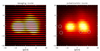 |
Fig. 6. Raw counts for the central 40 × 40 pixel regions of the Hα images for the central R Aqr binary, separation 45 mas, taken in imaging mode (left) and in polarimetric mode (right). The dotted circles in the polarimetric data indicate spurious charge shifting effects. |
The extracted subframes (even/odd or illuminated/covered rows) have an unequal dimension with twice the number of pixels in the row direction. The raw frames can be converted into a 512 × 512 pixel square format by a two pixel binning in row direction or into a 1024 × 1024 pixel square format by inserting everywhere between two adjacent rows one additional row with a flux conserving linear interpolation in column direction.
The pixel scale for even/odd or the illuminated/covered subframes are about 3.6 mas in row direction and 7.2 mas in column direction. The two pixel or Nyquist sampling in column direction is therefore 14.4 mas and this corresponds to the diffraction limit of the VLT telescope λ/D at a wavelength of 570 nm. However, the spatial resolution achieved with ZIMPOL is typically above 20 mas because of telescope and instrument vibrations, optical aberrations and other effects, so that the pixel sampling in column direction is also adequate for the shortest wavelength filter V_S (532 nm). Nonetheless, it can be beneficial for the data analysis to arrange interesting structures of the target along the better sampled row direction, like the close binary in Fig. 6.
2.3.1. Detector modes
Three detector modes are fully characterized and tested for ZIMPOL, one for imaging and two for imaging polarimetry. Important parameters for these modes are given in Table 4. The imaging and the fast polarimetry modes are conceived for high contrast observations of bright stars and the slow polarimetry mode for longer integrations of images with lower illumination levels.
Parameters for the ZIMPOL imaging and polarimetric detector modes.
The two ZIMPOL detectors are controlled for all detector modes strictly in parallel. The CCDs are operated as frame transfer devices where read-out of a frame in the shielded read-out area occurs during the integration (and demodulation in polarimetric mode) of the next frame in the imaging area (Schmid et al. 2012). Therefore, the shortest possible integration  is essentially the read-out time for one frame. After the integration a frame is shifted with a fast frame transfer from the image area to the read-out area and a new cycle of integration and read-out starts. The fast frame transfer introduces a small detector overhead of tft per frame and a smearing of the image which can be easily recognized as trails in column direction in short integrations of bright or saturated point sources (see Fig. 8). ZIMPOL includes a fast shutter to suppress the frame transfer smearing but it has been disabled because of technical problems. The ZIMPOL design does not require a shutter for the basic instrument-break modes.
Table 4 lists the electronic parameters for the different CCD modes, like read-out noise (RON), dark current (DC), and pixel gain. RON and DC need to be measured regularly for the calibration of the science data. The two CCDs are read out each by two read-out registers, one for the left half and the other for the right half of one detector. Each read-out register has a slightly different bias level which can vary by a few counts from frame to frame if the device is run with high frame rates. For this reason, the read-out registers provide for each half row also 25 pre-scan and 41 overscan pixel readings for each frame to correct properly the bias level in the data reduction. The raw frame format resulting from this read-out scheme is described in Schmid et al. (2012).
The standard imaging detector mode provides fast read-out and a high pixel gain of 10.5 e− ADU−1. The read-out noise is about 2 ADU pix−1, but because of the high gain this corresponds to a rather large RON ≈ 20 e−. Therefore, the standard imaging mode is not ideal for low flux observations and a low RON imaging mode for faint targets should be considered as a possible future detector upgrade. At the moment one can use the slow polarimetry mode as low-RON imaging mode.
A key feature of the polarimetric detector modes is the charge up and down shifting with a cycle period of Pmod = 1/νmod = 1.03 ms for fast or Pmod = 37 ms for slow modulation.
Fast modulation is designed to search for polarized sources, for example planets or disks, near (< 0.3″) bright stars with short integration times (≈1 − 5 s), high gain, and a deep full well capacity for collecting many photo-electrons per pixel (> 105) for high precision polarimetry. The modulation between I⊥ and I∥ is faster than the typical atmospheric coherence time τ0 ≈ 2 − 5 ms for medium and good seeing conditions ( ≲ 1″) at the VLT and therefore it is possible to suppress the speckle noise and reach a polarimetric sensitivity level at the photon noise limit of up to 10−5. Such a performance can only be reached if ≈1010 photo-electrons can be collected per spatial resolution element with a diameter of about 28 mas, or a synthetic aperture with ≈50 pix2 per detector what requires n > 1000 well exposed frames. Therefore, the fast modulation mode is tuned for short detector integration times tDIT < 10 s and high exposure levels > 1000 e− pix−1 for which the high read-out noise RON ≈ 20 e− pix−1 is not limiting the performance. The fast modulation mode produces a fixed bias pattern consisting of two pixel columns with special bias level values because the read-out of a pixel row must be interrupted to avoid interference with the simultaneous charge shifting in the image area. The pattern can be removed with a standard bias subtraction procedure (see Schmid et al. 2012).
The slow modulation mode is conceived and useful for polarimetry of sources around fainter stars or with narrow filters. This mode provides a slow modulation, but allows long integration times ≥10 s and delivers data with low RON ≈ 2 − 3 e− pix−1 appropriate for low flux levels.
2.3.2. Charge traps in polarimetric imaging
The up and down shifting of charges during the on-chip demodulation causes single pixel effects due to charge traps. This anticipated problem was minimized with the selection of CCDs with a charge transfer efficency of better than 99.9995%. A charge trap can hold for example one electron during a down shift and then release it in the following up-shift. In this way a trap can dig after 1000 shifts a hole of 1000 e− in the subframe of one modulation state, e.g. I⊥, and produce a corresponding spike in the I∥ subframe. A few examples are marked in the polarimetric frame of Fig. 6. This problem is solved with a phase switching in which the charge shifting is reversed in every second frame with respect to the polarization modulation. With such a double phase measurements one can construct a double difference
 (5)
(5)
for which the charge trap effects are cancelled or at least strongly reduced in the polarization signal (Gisler et al. 2004; Schmid et al. 2012). Io and Ie are the counts registered in the odd and even detector rows for either the zero (z) or π phase shifts between modulation and demodulation. In ZIMPOL, the alternating phase shifts are implemented automatically for polarimetric detector integrations and therefore only even number of frames can be taken per exposure. The charge trap effects increase with the number of modulation cycle and they are therefore small for short integrations tDIT and slow modulation mode. Unfortunately, the charge trap effects are not corrected for the intensity signal I = I⊥ + I∥ obtained with polarimetric imaging, and the affected pixels must be treated and cleaned like “bad” detector pixels.
2.3.3. The polarimetric modulation-demodulation efficiency
The ZIMPOL modulation-demodulation efficiency ϵmod is regularly measured with a standard calibration procedure (p_cal_modeff). This calibration takes fully polarized P = I⊥ = I 100 (I∥ = 0) flat field illumination using the calibration lamp in front of SPHERE and the polarizer in the ZIMPOL filter wheel FW0. The calibration measures either the mean fractional polarization ϵ = ⟨P Z/I⟩ or a 2-dimensional efficiency frame

The efficiency ϵmod is less than one because of several static and temporal effects which depend on many factors, mainly on the modulation frequency and the detector arm, but also on wavelengths (or filter) and on the location on the detector.
On the masked CCD, there is a leakage of photons and newly created photo-charges from the e.g. I⊥-subframe in the illuminated pixel rows to the adjacent covered pixel rows of the I∥ subframe, of about δstatic ≈ 5%. This reduces the efficiency by the factor ϵstatic = 1 − 2δstatic ≈ 0.9. The effect is slightly field dependent because the alignment of the stripe mask with the pixel rows, and therefore the leakage to the covered rows, is not exactly equal everywhere on the detector.
The polarization beam splitter is essentially perfect for the transmitted light in arm1, while about δarm2 ≈ 3% of the “wrong” I∥ intensity is deflected together with I⊥ into arm2. This reduces the relative efficiency of arm2 by ϵarm2 = (1 − δarm2)/(1 + δarm2)≈0.94.
For fast modulation a temporal efficiency loss occurs because a finite time of about 75 μs is required for the FLC modulation switch and the CCD line shift. This reduces the modulation-demodulation efficiency of ZIMPOL by about 10% or ϵtemp ≈ 0.9 for the fast modulation mode. For slow modulation the temporal effect can be neglected.
It results a ZIMPOL overall polarimetric efficiency of about ϵmod ≈ ϵtempϵstatic ≈ 0.8 for fast modulation polarimetry and ϵmod ≈ ϵstatic ≈ 0.9 for slow modulation polarimetry with arm1. For arm2 an additional factor of ϵarm2 ≈ 0.95 needs to be included (see Bazzon et al. 2012; Schmid et al. 2012, for further details).
The fast frame transfer (with open shutter) causes also a reduction of the measured efficiency for the measured fractional polarization PZ/I. During the frame transfer the detector is still illuminated and the intensity I⊥/2 + I∥/2 is added during the frame transfer time tft to both, the I⊥- and I∥-subframes. This reduces for a polarized flat-field illumination, or a full frame aperture measurement like for a standard star, the fractional polarization PZ/I by
 (6)
(6)
The frame transfer effect is stronger for short integration times in fast modulation. The factor is ϵft = 0.973, 0.986, and 0.995 for integration times of tDIT = 2 s, 4 s, and 8 s (and tft = 56 ms). For slow polarimetry with tft = 74 ms there is ϵft = 0.993 for  s and higher for longer integrations.
Table 5 gives the mean values from many calibrations taken throughout the year 2015 for ϵftϵmod = PZ/I, while ϵmod are the efficiencies corrected for the transfer smearing according to Eq. (6). The calibrations show clearly the ϵmod-differences between cam1 and cam2 and between fast and slow modulation in particular with the ratios given in the last column and the bottom row. The N_R data taken with tDIT = 4 s, 2 s, and 1.1 s illustrate well the ϵft dependence. The efficiency ϵmod shows also a small dependence on wavelength. The efficiencies ϵmod given in italics are recommended values for a particular camera, modulation mode, and filter. The statistical uncertainties in the ϵmod calibrations are less than σ < 0.005 as derived from sets of four or more measurements taken during 2015 with the same instrument configuration. Thus, the ϵmod calibrations are very stable for a given configuration and the obtained values or calibration frames are valid for a month typically and possibly even longer.
Calibration measurements taken during the year 2015 for the modulation – demodulation efficiencies ϵftϵmod and ϵmod in various filters.
The degradation of the polarization flux because of the non-perfect (< 1) modulation-demodulation efficiency of ZIMPOL is corrected with a calibration frame ϵmod(x, y) according to
 (7)
(7)
which we call polarmetric correction “c1”. This type of correction considers also the field dependent detector effects but might also introduce pixel noise from the calibration frame if not corrected. For not very high signal to noise data P/ΔP < 50, it is good enough to correct the PZ(x, y) just with a mean value ⟨ϵmod⟩ as given in Table 5. For the derivation of the fractional polarization PZ/I in a large aperture one needs also to account for the frame transfer illumination by using ϵmodϵft.
2.4. ZIMPOL filters
The pass bands of the available ZIMPOL color filters are shown in Fig. 7 and listed in Table 6 with central wavelengths λc, filter widths Δλ (FWHM), their location in the filter wheels, and whether they can be combined with the dichroic beam splitter or with one of the two coronagraphic four-quadrant phase masks 4QPM1 or 4QPM2 (see Sect. 4). Table 6 includes also the calibration and test components in the filter wheels.
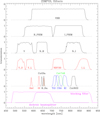 |
Fig. 7. Transmission curves for the ZIMPOL color filters, the blocking filter and the dichroic beamsplitter. Black curves are used for filters located in FW1 and FW2, red for filters in FW0, blue are filters in FW1 only, and green filters in FW2 only. |
Pass-band filters, neutral density filters, and calibration components available in the filter wheels FW0, FW1 and FW2 of ZIMPOL.
The ZIMPOL filters were selected based on several technical and scientific requirements:
For imaging, all pass band filters can be used. The filters in FW1 and FW2 can be combined with one of the three neutral density filters located in FW0 to avoid image saturation. One can use the same filter type in FW1 and FW2 to optimize the sensitivity in that pass band or one can also use simultaneously two different filters in FW1 and FW2. The latter mode provides spectral differential imaging, e.g. combining an Hα filter with the continuum filter CntHa. Alternatively, using different filters provides an efficient way to get angular differential imaging with large field rotation in two pass bands simultaneously, e.g. R_PRIM and I_PRIM, during one single meridian passage of a target.
When combining different filters in FW1 and FW2 it needs to be considered that the detector integration times are equal in both channels. Broad-band filters combined with narrow band filters can therefore cause strongly different illumination levels on the two detectors.
The filters in FW1 and FW2 are recommended for polarimetry, because they are located after the polarization beam-splitter and the polarization is encoded as intensity modulation. Therefore, polarization dependent pass bands and other polarization effects of the filters do not affect the polarization measurements. Only for these filters a modulation-demodulation efficiency ϵmod can be determined, because this calibration requires the polarizer located in FW0. Polarimetry using the neutral density filters or the color filters in FW0 is also possible but with an increased polarimetric calibration uncertainty. More work is required to characterize accurately such non-optimal polarimetric modes.
Different filters can be used in FW1 and FW2 simultaneously for ZIMPOL polarimetry, because each arm provides a full polarization measurement. Thus one can perform a combination of simultaneous spectral and polarimetric differential imaging with ZIMPOL.
There are some instrument configurations which can only be combined with certain filters. Observations with the dichroic beam-splitter between ZIMPOL and WFS provide more photons for the WFS and is therefore particularly beneficial for faint stars. This mode must use the filters N_R, B_Ha, N_Ha, NB_Ha, CntHa, and OI_630, which have their pass bands in the transmission window of the dichroic BS plate (Table 6, Col. 7). The R-band four quadrant phase mask coronagraph 4QPM1 has its central working wavelength at 650 nm and is also designed for these filters. The I-band 4QPM2 with central wavelength 820 nm requires the filters Cnt820 or N_I for good results (Table 6, Col. 8).
The following list gives important scientific criteria which were considered for the selection of the different filters:
-
V, N_R and N_I broad band filters for imaging and polarimetry of stars and circumstellar dust,
-
RI (or VBB for very broad band), R_PRIM, and I_PRIM broad band filters for demanding high contrast observation where a high photon rate is beneficial for the detection,
-
TiO_717, CH4_727, KI, Cnt748 and Cnt820 for narrow band imaging, spectral differential imaging and polarimetry of cool stars, substellar objects and solar system objects,
-
B_Ha, N_Ha and CntHa for imaging, spectral differential imaging, and polarimetry of circumstellar Hα emission,
-
V_S, V_L, 730_NB, I_L for better coverage of the ZIMPOL spectral range with intermediate band filters,
-
OI_630 and HeI as additional line filters for the imaging of circumstellar emission,
-
N_R, the Hα filters B_Ha, N_Ha (NB_Ha), CntHa, and OI_630 in combination with the dichroic beam splitter for imaging, differential imaging and polarimetry of fainter targets R ≳ 9 mag, where the AO performance profits from the higher photon throughput to the wave front sensor.
Blocking filter. A problem of the pass band filters is their insufficient blocking of the transmission (often not less than 0.001) for wavelengths outside the ZIMPOL range λ < 500 nm and λ > 900 nm. This can be particularly harmful for coronagraphic observations, where radiation from the central, bright source is displaced for wavelengths outside the ZIMPOL spectral range, because the atmospheric dispersion corrector is not designed to correct for these wavelengths. For coronagraphic images some of the central star radiation, e.g. the blue light (420 − 480 nm), might not fall onto the focal plane mask. This would create a point like signal slightly outside the mask despite an out-of-band attenuation of ND ≈ 3 of the color filter. For this reason a blocking filter is added on the “free” position of the modulator slider for imaging, and one is added to the entrance window of the modulator vacuum housing for polarimetry.
3. The AO corrected point spread function
The PSF obtained with SPHERE/ZIMPOL are complex and depend on wavelengths, atmospheric conditions, star brightness and observing modes. This section describes characteristic PSF parameters for many different cases.
3.1. Two-dimensional PSF structure
Figure 8 shows the averaged PSFs of HD 183143 in the V-band and the N_I band for 48s of integration each taken on 2015-09-18, the N_I-frames about 2 min after the V-frames. These are “typical” PSFs for a bright star and for stable and good atmospheric conditions.
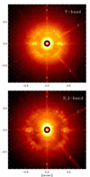 |
Fig. 8. Normalized PSFs of HD 183143 for the V-band (top) and the N_I-band (bottom) with the color scale reduced by a factor of 100 for the central peak within r < 20 pixels. Marked PSF features are the speckle ring near the AO control radius (r), strong fixed speckles from the AO system (s), two telescope M2 spider features (t), and the CCD frame transfer trail of the PSF peak (c). The dashed rings illustrate the location of the azimuthal cuts shown in Fig. 9. |
The polarimetric mode P1 with derotator fixed was used, and the PSF is displayed in the orientation of the detectors with x and y in row and column directions, respectively. The corresponding polarization images for the V-band PSF are discussed in Sect. 5.5.
Prominent PSF features in Fig. 8 are the strong speckle ring at a spatial separation corresponding roughly to the AO control radius of rAO = 20 λ/D up to which the AO corrects the “seeing” speckles. This corresponds to ρAO ≈ 0.3″ for the V-band and ρAO ≈ 0.45″ for the N_I-band. Dashed rings indicate azimuthal cuts through the PSF, which are shown in Fig. 9. Strong quasi-static speckles from the AO system, marked with “s”, are always present left and right from the PSF peak on the speckle ring near r = 80 pix for V and r = 120 pix for N_I. Another feature of the PSF are the diffraction pattern of the four spiders holding the M2 telescope mirror and two of the four appear particularly bright in Fig. 9. The vertical line through the PSF peak is the frame transfer trail, which is caused by the illumination of the detector during the fast frame transfer. The trail is particularly strong for non-coronagraphic observations of bright stars with short integrations (see Eq. (6)).
 |
Fig. 9. Azimuthally averaged radial profiles ctn6( ρ) (left) and azimuthal profiles ctn6(r, ϕ) for r = 50, 80, 120 and 180 pix (right) corresponding to ρ = 0.18″, 0.29″, 0.43″, and 0.65″, respectively for the PSFs of HD 183143 shown in Fig. 8. Also indicated as gray shading are the standard deviations of the azimuthal points σ(ctn6(r, ϕ). The location of the azimuthal cuts are indicated in the ct6n(r)-panels and in Fig. 8. |
Figure 9 gives averaged radial profiles and azimuthal cuts of the PSF for a more quantitative description. The PSFs in Figs. 8 and 9 are given in units of ctn6 where the counts are normalized to 106 counts within a round aperture with a diameter of 3″. The normalization of the surface brightness SB [mag arcsec−2] of a PSF to the total stellar flux mstar [mag] defines a normalized surface brightness or a surface brightness contrast CSB [mag arcsec−2] according to:
 (8)
(8)
This translates, for the applied PSF normalization of 106 ct in the 3″-aperture, to the following normalized surface brightness conversion between ctn6 [pix−1] and mag arcsec−2
 (9)
(9)
using −2.5m log(77160/106)= + 2.78m because one arcsec2 contains 77160 pixels on one ZIMPOL detector. Thus, a PSF peak surface brightness of ctn6(r = 0)=5000 ct pix−1 corresponds to a normalized surface brightness of CSB(0)= − 6.47 mag arcsec−2. A signal of 1 ctn6 for example from a faint companion with a point source contrast of about Δm ≈ 9.25m, is at the level to be visible for r ≳ 80 pix in the normalized images and cuts shown in Figs. 8 and 9 except for the regions of the speckle ring.
The radial PSF profiles in Fig. 9 show the azimuthal mean with the standard deviation ±σ indicated in gray. Four radii were selected to show the azimuthal profiles ctn6(r, ϕ) of the PSF as function of position angle ϕ measured counterclockwise from top. The innermost ring profiles r = 50 pix show a sine-like pattern, especially for the N_I band, with two maxima and minima within 360°. They originate from the slightly elongated base of the very strong ctn6(0) ≈ 5000 ct pix−1 PSF peak (see also Fig. 11). Such PSF extensions are often present and they can be caused by a dominant wind direction.
The speckle rings at r ≈ 80 pix in the V-band and at r ≈ 120 pix for the N_R band produce very strong noise features on small angular scales. The strongest speckles are at 90° and 270° degrees from the AO system as already discussed above (Fig. 8). Speckles are weaker inside the speckle ring and outside they are hardly recognizable besides the faint traces from the spiders at ϕ = 220° and 300° and the frame-transfer trail at 0° and 180°. Because of the location of the speckle rings the N_I-band observations would be much more sensitive in the radial range 0.2″–0.4″ than V-band observations. On the other side a faint target at a separation between ρ = 0.4″−0.5″ might be easier to detect (assuming gray color distributions) just outside the speckle ring in the V-band than on the speckle ring in I-band.
The dominant noise sources are the distortions close to the center, the strong speckles further outside, and the read-out noise outside of the control ring. The read-out noise regime can be pushed outwards easily with a stronger frame illumination, where the PSF peak is saturated or close to saturation, or with coronagraphic observations.
3.2. Parameters for the radial PSF
To simplify our discussion we focus on the radial profiles of the PSF keeping in mind the significant deviations from rotational symmetry discussed above (Figs. 8 and 9). We use as basis for this brief overview the polarimetric standard star data from the ESO archive taken in polarimetric mode in the V, N_R, N_I band filter, which are regularly obtained by ESO staff as part of the SPHERE instrument calibration plan. In addition we include a few special PSF cases. As a starting point, we have selected the data of HD 183143 from Sept. 18, 2015 (Figs. 8 and 9) as typical examples of SPHERE/ZIMPOL PSFs for the V, N_R and N_I-band taken under good atmospheric conditions.
PSF wavelength dependence. Figure 10 compares the flux normalized radial profiles ctn6(r), with equally normalized diffraction limited profiles f(r)/f3dia calculated for the VLT with an 8.2 m primary mirror and a 1.1 m central obscuration by the secondary mirror and where f3dia is the total flux within an aperture with a diameter of 3″. Also shown is the H-band (1.62 μm) diffraction profile. For each filter f(r) is the mean PSF for several wavelengths equally distributed over the filter range to account for the filter widths.
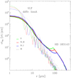 |
Fig. 10. Flux normalized PSFs ctn6(r) for HD 183143 (thick profiles) and the calculated diffraction limited PSF of the VLT (thin profile) for the filters V (λ = 545 nm), N_R (645 nm), N_I (817 nm), and including the H-band (1.62 μm) for the VLT. One pixel is 3.6 mas. |
The normalized peak flux ctn6(0) for HD 183143 (Fig. 10) are roughly at the same level for all filters. The most prominent difference between the PSFs is the wavelength dependence for the radius of the local maximum associated with the speckle ring. Contrary to the observed profiles the peak flux of the normalized VLT diffraction PSFs depend strongly on wavelength. For the pixel size of 3.6 × 3.6 mas2 there is f(0)/f3dia = 5.13%, 3.80%, and 2.36% for the V, N_R, and N_I filters, respectively (see bottom lines in Table 7).
PSF characteristics for three typical standard stars and several special cases.
We use the normalized peak flux ctn6(0) as key parameter to compare the PSF quality of different SPHERE/ZIMPOL observations. This value can be determined easily and under good atmospheric conditions similar values in the range 0.4−1.0% are obtained for different wavelengths.
For a comparison with the performance of other instruments one should translate the peak flux into a Strehl ratio. An approximate Strehl ratio S0 can be calculated with the relation
One should note, that a lower Strehl ratio at shorter wavelengths is not equivalent with a lower normalized peak flux because the diffraction peak depends strongly on wavelength, like f(0)/f3dia ∝ 1/λ 2.
The approximate Strehl ratio S0 provides a useful parameter for a simple assessment of the SPHERE/ZIMPOL system PSF. However, the S0 value does not describe well the SPHERE AO performance, because there exist instrumental effects which degrade the PSF peak which are not related to the adaptive optics (as discussed in Schmid et al. 2017). A more sophisticated AO characterization should be based on the analysis of the Fourier transform of the aberrated image as described in Sauvage et al. (2007). Such an analysis yields for the N_I-filter PSF of HD 183143 an AO Strehl ratio of 33% instead of the 23% resulting from the values given in Table 7. The difference can be explained by a residual background at low spatial frequencies caused for example by instrumental stray light, not corrected frame transfer smearing, and other effects.
Figure 11 shows the peak normalized PSF of HD 183143 for the three filter on a linear scale. The PSF full width at half maximum (FWHM) are significantly larger, by about 2 − 3 pixels or 7–11 mas, when compared to the diffraction limited profile (Table 7). Different effects contribute to this degradation like small pointing drifts, residual PSF jitter because of telescope and instrument vibrations, residuals from the atmospheric dispersion correction and other uncorrected optical abberations, cross-talks between detector pixels, and possibly more. Also shown in this plot are the maxima of the speckle rings. The mean profiles can be misleading when considering the strong azimuthal dependence discussed in Fig. 9.
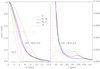 |
Fig. 11. Same PSFs for HD 183143 and the VLT diffraction limit as in Fig. 10 but normalized to the peak flux. The dashed line in the left panel marks the half width at half maximum of the profiles. The dotted curves are the calculated diffraction limited profiles. The flux scale in the right panel is 100 times lower. |
The profiles of the normalized encircled flux Ef(r) shown in Fig. 12 is another way to characterize the PSFs. This plot illustrates that only about 20% of the total PSF flux is encircled in an aperture with r = 5 pix (18 mas), or about 30% for r = 10 pix. The encircled flux is an important parameter for flux determinations using synthetic apertures. We select as characteristic parameter the halo and background corrected encircled flux Ef10 for an aperture radius of r = 10 pix, using the mean flux value ⟨ctn6(r = 11)⟩ of the pixel ring with r = 11 pix as background and halo level, which is subtracted from all 317 pixels i within the aperture ri ≤ 10 pix
![Mathematical equation: $$ \begin{aligned} E_{f10} = {1\over 10^6} \sum _{r_i\le 10}\bigl [{\mathrm{ct}_{\rm n6}(x_i,y_i) -\langle \mathrm{ct}_{\rm n6}(r=11) \rangle }\bigr ]. \end{aligned} $$](/articles/aa/full_html/2018/11/aa33620-18/aa33620-18-eq19.gif) (10)
(10)
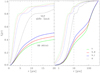 |
Fig. 12. Profiles for the normalized encircled flux Ef(r) for the same PSFs of HD 183143 and the VLT diffraction as in Fig. 10. The dashed lines illustrate the parameter Ef10. |
This type of encircled energy measurement is also applicable to the PSF peak of faint companions, for which it is not possible to measure the outer part of the PSF. For high contrast measurements we need Ef10, or encircled energies for other apertures with small radii, to derive the flux contrast between central star and faint companion. The measured Ef10-values for HD 183143 and other test cases are given in Table 7.
3.3. PSF variations
The PSFs obtained with SPHERE/ZIMPOL show a large diversity depending on atmospheric conditions, central star brightness, AO performance, and instrumental mode, and a few typical cases are discussed in this subsection. Table 7 lists for the analyzed profiles the measured PSF values for the normalized peak flux ctn6(0), the encircled energy Ef10, and full width at half maximum FWHM. Also given are atmospheric and instrument parameters taken from the ESO data file headers. Seeing and coherence time τ0 are measured for the vertical direction with the DIM-MASS systems.
Atmospheric conditions. The PSF of SPHERE/ZIMPOL changes often strongly within one night and under instable conditions even from frame to frame. Figure 13 compares for bright standard stars the typical or “good” PSFs of HD 183143 for the V-band and the N_I band with the “excellent” PSFs of observations of HD 161096 and the “bad” PSFs of HD 129502. These three examples represent quite well the much larger data set of bright standard stars available in the ESO archive. These archive data show an overall correlation between good PSFs parameters and long atmospheric coherence times scales τ0 ≳ 3 ms or good seeing ≲0.9″ and bad PSFs for short time scales τ0 ≲ 2 ms or mediocre seeing ≳1.0″. This is roughly in agreement with the study of Milli et al. (2017) on SPHERE PSF properties in the near IR. Bad atmospheric conditions as for the observations of HD 129501, affect much more the short-wavelength V-band profile. Other effects, for example the high airmass for the observations of HD 183143, play also a role.
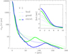 |
Fig. 13. Normalized radial profiles ct6n for V- and N_I-band observations of HD 161096 with “excellent”, for HD 183143 with “good”, and HD 129502 with “bad” quality PSFs. |
Let us consider in more detail the contrast characteristics of the three N_I profiles bad, good, and excellent in Fig. 13 and Table 7. Normalized peak fluxes and encircled fluxes scale roughly like 0.7 : 1.0 : 1.4 between bad : good : excellent conditions. The normalized mean flux level at r = 80 pix is much lower ≈1.5 ct for the “excellent” PSF, and ≈5 ct for the “good” and “bad” PSF. The speckle noise is measured as standard deviation of fluxes in apertures at r = 80 pix (0.29″) as illustrated for the case of α Hyi B in Fig. 21a. This yields the 5-σ raw contrasts for the faint point source detection at ρ = 0.29″ of about 8 × 10⁻⁴ : 4 × 10⁻⁴ : 2.3 × 10⁻⁴ for the bad : good : excellent PSFs discussed here.
This rough estimate does not consider differential imaging techniques for speckle noise suppression, which may change the picture. In any case, there exist dramatic differences of factors 2 − 4 in the SPHERE/ZIMPOL contrast performance for bad, good or excellent atmospheric conditions which are of great importance when defining the seeing requirements for observations of a particular object.
Low wind effect. The PSF of HD 142527 in Fig. 14a is an extreme example for the so called low wind effect, which leads to multiple PSF peaks in the center. This is explained in Sauvage et al. (2016a) by a discontinuity in the wave front phase in the pupil plane at the location of the mirror M2 telescope spiders. These spiders are cold and cause a temperature difference between the air in upwind and downwind direction. Such phase offsets are not easily recognized by the Shack-Hartmann WFS and therefore different PSF peaks result. This effect is only observed when the wind is particularly slow, ≲2 m s−1, so that the heat exchange between spider and air induces a substantial temperature difference. The atmospheric conditions for the observation of HD 142527 were in principle excellent with a very good seeing of 0.65″ and a long coherence time of 11.5 ms, but a wind speed of only 1.5 m s−1 (Table 7). The FWHM is 53 mas for the multiple peaked PSF and the relative peak flux ctn6(0) is a factor 2.5 − 4.0 lower than for other PSFs taken under sub-arcsecond seeing conditions.
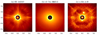 |
Fig. 14. Normalized PSFs for special cases: Panel a: VBB-filter image of HD 142527 as example for the low wind effect, panel b: faint star 47 Tuc MMS12 in I_PRIM, and panel c: a 10 ms snap-shot image of α Eri A and B in the line filter CntHa. The color scale is reduced by a factor of 100 for the PSF center within ρ < 0.072″. Axes are in arcsec. |
Still relatively high is the encircled energy Ef10 = 35%, which is comparable to “good” atmospheric conditions. Thus the low wind effect splits the central PSF peak and degrades the resolution, but at larger separation the Ef(r)-profile is not much affected. This means that the sensitivity for high contrast imaging of extended circumstellar scattering regions is not strongly degraded by the low wind effect, apart from the reduced spatial resolution. For example, the ZIMPOL observations of the proto-planetary disk around TW Hya described by van Boekel et al. (2017) suffered from the low wind effect, but despite this the quality of the resulting disk images is good and certainly competitive with near-IR observations from other AO instruments (Akiyama et al. 2015; Rapson et al. 2015).
Central star brightness and color. The AO performance degrades for faint stars, because of the lack of photons for accurate measurements and corrections of the wave front distortions. In addition the WFS shares the photons in the “visual” range 500 − 900 nm with the ZIMPOL science channel. The gray beamsplitter (zw.BS) reflects only 21% of the light to the WFS and therefore the AO performance degrades significantly for stars fainter than about R ≈ 8m (see Sauvage et al. 2016b). This limit is relaxed to about R = 9.2m, if the dichroic beam-splitter is used instead of the gray beam splitter, but then the useful spectral range for ZIMPOL is reduced to the N_R-filter and the line filters B_Ha, N_Ha, CntHa and OI (see Fig. 7). For faint central stars there are means to optimize the AO system with longer integrations with the WFS camera, running with reduced AO-loop frequencies of 600 Hz or 300 Hz instead of 1200 Hz, and the use of a large spatial filter in the WFS arm (see Sauvage et al. 2016b). A mirror instead of a beam splitter is used for infrared science observations and therefore more light reaches the WFS and the corresponding limit is about R ≈ 10.0m.
Figure 14b shows as example for a faint star the central regions of 47 Tuc MMS12, the central star of the astrometric field from Fig. 3. This star has only R = 10.5m and was observed with the gray beam splitter under mediocre atmospheric conditions at high airmass and therefore the resulting PSF is strongly downgraded. When compared to the N_I band PSF of the bright HD 129502, which was observed under similar seeing conditions, then the faint star in 47 Tuc MMS12 has a 10× lower normalized peak flux (or Strehl ratio), 3× lower encircled flux Ef10, and a 2× enhanced FWHM (Table 7). Figure 3 demonstrates that the resulting image can still be useful, but the broad and extended PSF is strongly reducing the spatial resolution and the contrast performance, and produces a much higher read-out noise limit for faint stars.
The AO-correction may also depend on the color of the central star. A strong wavelength dependence of the PSF parameters is reported by Schmid et al. (2017) for the Mira variable R Aqr with very red colors V − I = 7m. The normalized peak counts ctnb(0) show a strong wavelength dependence with 0.54% for the I-band but only 0.09% for the V-band (Table 7). The explanation is most likely, that the WFS “sees” essentially only I-band light, because of the very red color of the star, and therefore the AO-system performs less good in the V-band.
PSF structure and instrument mode. A few special instrumental effects are noticeable in the PSFs shown in Fig. 14a and c.
Figure 14a shows the PSF of the star HD 142527 taken with the VBB filter with a filter widths of Δλ = 290 nm for a central wavelength of λc = 735 nm or λc/Δλ = 2.53. In this case the speckles are strongly extended radially. This has the disadvantage that the ring of bright speckles is very broad, but on the other side the flux of an individual speckle is distributed over many pixels and therefore the elongated speckles are less prominent, and they can be distinguished more easily from a faint point source companion.
The star α Eri A with its fainter companion α Eri B were taken during the SPHERE commissioning with the narrow line filter CntHa with a very short integration of 10 ms using the “snap shot” engineering mode of the ZIMPOL detector, and a single 10 ms exposure is shown in Fig. 14c. For our data we measure for the companion a relative separation of 175 ± 4 mas, a sky position angle of −19.5 ° ±2.0°, and a flux ratio of about fB/FA = 0.014. This position measured by us for 2014-10-13 (2014.78) coincides with the location for epoch 2007.75 in the partial orbit measured by Kervella et al. (2008), indicating an orbital period of about 7.0 ± 0.1 yr for the α Eri binary. Because of the narrow filter and the very short integration the speckles are strong and point like because there is no or only little radial and temporal smearing, respectively. For averaged PSFs or PSFs taken with long integration times like in Fig. 8, the pattern of the strongly variable speckles will average out and only strong quasi-static speckles remain clearly visible. We note, that the PSF parameters given in Table 7 are derived from averaged PSFs of nDIT-images where the PSF of each image was re-centered individually before adding it to the others.
The PSF peak for α Eri is very narrow, because slow instrumental drifts and vibrations with frequencies < 100 Hz do not broaden the PSF peak in very short integration. Further, there is no spectral dispersion because the line filter CntHa produces essentially monochromatic images. For these reasons, the PSF of α Eri has a FWHM of ≈19 mas, which is about 1 pixel better than for the observations taken under “excellent” conditions or 2 pixels better than for “good” conditions (Table 7).
Not corrected instrumental vibrations can also be recognized in the frame transfer trails of a bright source. These trails wiggle left and right with a scatter of σ ≈ 1 − 2 pix from the mean position and one such excursion extends over about 200 pixels in vertical direction corresponding to a time scale of 10 ms during the frame transfer. This residual PSF jitter explains partly the discrepancy of 2−3 pix between observed widths of the PSF peak and the nominal width of a diffraction limited PSF profile.
Lucky imaging and speckle suppression techniques can be optimized with a careful selection of instrument and observing parameters, which enhance or reduce the speckle variations between frames or which modify the geometric appearance of speckles (e.g. Law et al. 2009; Brandner et al. 2016). It is beyond the scope of this paper to investigate further such techniques apart from pointing out that ZIMPOL offers a broad range of instrument modes which can be exploited.
4. Coronagraphy
Coronagraphy is a powerful tool to suppress the light of a bright object for the search of faint sources at small separation (Malbet 1996; Sivaramakrishnan et al. 2001). The basic concept of the SPHERE visual coronagraph is a classical Lyot coronagraph where the focal plane mask stops the light of the bright star and the pupil mask stops the diffracted light from the telescope and the coronagraph in a pupil plane further downstream. SPHERE has a focal plane exchange wheel with 16 positions equipped with 7 round focal plane masks, 2 monochromatic four quadrant phase masks (4QPM), two open field stops (see Table 8), and 4 empty positions. There is also an exchange wheel with 8 positions for pupil stops (Table 9).
Focal plane masks in the SPHERE visual coronagraph.
Geometric parameters for the telescope pupil, the intermediate pupil, and the pupil stop masks in the SPHERE visual coronagraph.
The F-ratio of the coronagraph is F#=30 and the pupil size in the collimated beam is 6 mm in diameter. The focal plane masks serve also as field stop for ZIMPOL defining either a circular “wide field” (WF) with a radius of ρ = 4″ or a “narrow field” (NF) of 1″×1″ for a very fast, windowed detector read-out mode for polarimetry, which was not commissioned yet.
We use the stellar system α Hyi (HR 591, HIP 9236) as a test target for the on-sky characterization of the SPHERE visual coronagraphs. α Hyi is a bright mV = 2.9m, nearby (22 pc), F0 star and was used as test target in the commissioning. It turned out to have a nearby companion which is ideal for the characterization of the SPHERE visual coronagraph. α Hyi B is not in the SIMBAD data base but the Hipparcos catalog gives for α Hyi a binary orbit for the astrometric photo-center motion with an orbital period of P = 606 days and a semi-major axis of 21.7 mas. On 2014-10-10 we measure a separation of 91 ± 3 mas and a position angle of −19 ° ±2°. The companion is about 5.8m ± 0.2m and 6.5m ± 0.2m fainter than the primary in the I_PRIM and R_PRIM bands, respectively (see Table 10).
Measurements of the flux ratio fB/fA and the (S/N)B of α Hyi A and B, using different coronagraphic configurations of SPHERE/ZIMPOL.
The atmospheric conditions for our coronagraph tests were photometric, with an atmospheric coherence time of about τ0 ≈ 2.8 ms and a seeing of roughly 0.83″ (see Table 7).
4.1. Coronagraphic focal plane masks
Figure 15 shows images of the central region (1.8″ × 1.8″) of nine focal plane masks obtained with flat-field lamp illuminations. For non-coronagraphic observations, the clear field stop NC_WF (or NC_NF for window mode) are used. Non-coronagraphic observations can also obtained by offsetting the star from the mask, but then a shadow from the coronagraph will be present in the image and the pupil stop is still in place. Such “offset PSFs” taken before or after coronagraphic observations are very useful for the flux calibration and the PSF characterization.
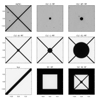 |
Fig. 15. Images of the central part (1.8″×1.8″) of focal plane masks available in the visual coronagraph of SPHERE. The masks in the top row are deposited on a plate and the gray scale is enhanced to show the frequency of dust features on the masks. |
Several Lyot coronagraphs with different spot sizes are available. Small spots, suitable for small inner working angles, are made of a metallic coating deposited on transparent plates with the disadvantage that dust particles on the plate are visible in the recorded images. In Fig. 15 the gray scale for CLC_S_WF, CLC_MT_WF (and 4QPM1) is enhanced to illustrate the frequency of such dust features as seen for our tests in Oct. 2014.
Larger coronagraphic spots are suspended with thin wires. Dust are no problem for these masks but the suspension spiders, which have a full width of 40 μm = 34 mas, can be an important issue for the observing strategy and the data reduction.
The coronagraphic attenuation of the PSF of α Hyi for the small CLC-S-WF, medium CLC-M-WF, large CLC-L-WF, and extra large CLC-XL-WF Lyot spots are shown for the I_PRIM filter data in Fig. 16 as coronagraphic images and in Fig. 17 as azimuthally averaged radial profiles. These coronagraphic data were taken simultaneously in the I_PRIM filter for cam1 and the R_PRIM filter for cam2 using the pupil stopB1_2. Figure 17 includes a stellar PSF taken with the star offset by 550 mas from the mask spot and using the neutral density filter ND2 to avoid heavy saturation. The non-coronagraphic PSF was normalized to 106 ct for an aperture with a diameter of 3″ and all the coronagraphic profiles were scaled to this ctn6-normalization considering the exposure times and the attenuation of the neutral density filter ND2 (about a factor 130 for R_PRIM and 105 for I_PRIM) used for the non-coronagraphic observations. The two last columns in Table 8 give the maximum counts of the ctn6-normalized images.
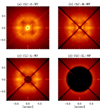 |
Fig. 16. Coronagraphic images of α Hyi (1.8″×1.8″) for the I_PRIM-filter taken with the panel a: small S, panel b: medium M, panel c; large L, and panel d: extra-large XL focal plane masks of SPHERE All images are normalized ctn6 relative to the non-coronagraphic PSF and displayed with the same color scale. |
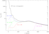 |
Fig. 17. Normalized radial profiles ct6n(r) for the I_PRIM coronagraphic images in Fig. 16 of α Hyi taken with the small S (blue), medium M (green), large L (red), and extra-large XL (magenta) focal plane stops. Also plotted is the non-coronagraphic PSF profile. The dotted lines indicate the nominal mask radii. |
Depending on the spot size different features of the PSF are attenuated. The smallest mask CLC-S-WF reduces the flux peak by about a factor Rcoro ≈ 110 − 150, which corresponds to the ratio of the max(ct6n)-counts between off-mask PSF and coronagraphic image given in Table 8. This mask leaves a ring of strong residuals at a separation of about 60 mas just outside the coronagraphic spot. The next larger mask CLC-MT-WF ( ρ = 81 mas) attenuates the central peak completely Rcoro ≈ 300 − 600, and the flux just outside the mask rim is comparable to the strong features in the speckle ring at ρ ≈ 0.3″−0.4″. For CLC-L-WF the speckles in the speckle ring are the strongest emission features, while for CLC-XL-WF also all bright speckles in the ring are hidden and the coronagraphic attenuation reaches Rcoro ≈ 1000−3000.
Very useful for the determination of the stellar position in the coronagraphic images, in particular for the large focal plane masks, are the interference features from the DM at ρ ≈ 0.6″−0.9″ above, below, left and right from the hidden star. They are essentially grating spectra of the central star created by the chessboard pattern from the DM actuators which can be recognized in the pupil image (see Fig. 19).
Another focal plane mask in the visual coronagraph is the astrometric mask CLC-MT-WF, which has a Lyot spot with a transmission of about 0.1%, so that the central star can be seen in the science image as a faint emission peak inside the spot shadow. This is very useful for astrometric measurements of circumstellar sources. This mask has no suspension wires which is an advantage when compared to CLC-M-WF. In addition, the mask has a Cartesian grid of smaller spots spaced by 1″ for the astrometric location of sources observed in off-axis settings where the central star is outside the detector field of view. A central spot is often also visible for the small opaque mask CLC_S_WF, but this spot is produced by diffraction and should not be trusted for astrometric purposes.
The four quadrant phase masks (4QPM) have a geometry as shown in Fig. 15 (top left). The plates produce a phase shift of π through a small optical path difference in the left and right quadrants with respect to the upper and lower quadrants introducing a destructive interference at the interfaces and a particularly efficient nulling for the central crossing (Rouan et al. 2000). The simple, monochromatic 4QPM used in ZIMPOL are designed for one wavelength λ0 and the attenuation is less efficient for wavelengths away from λ0 (Riaud et al. 2003). 4QPM1 with λ0 = 666 nm is designed for the N_R-band filter the Hα line filters B_Ha, N_Ha and CntHa. The 4QPM2 with λ0 = 820 nm is foreseen for the N_I filter and the narrow band filter Cnt820.
The bar mask could be useful for the search of faint objects near a small separation ( ρ < 2.5″) binary star. The orientation of the binary can be aligned with the bar in field stabilized mode with an offset of the field position angle. We have not tested the performance of this mask.
4.2. Pupil plane stops
An important part of classical Lyot coronagraphs and 4QPMs are pupil plane stops which suppress the light diffracted by the sharp edges of the telescope pupil and the coronagraphic mask in the focal plane (e.g. Sivaramakrishnan et al. 2001). In the coronagraph pupil the diffracted light is located in two bright rings, one just outside the central M2-mirror obstruction and one along the outer pupil edge. In the coronagraphic image the pupil masks reduce efficiently the strong inner diffraction rings and this effect is quantified in the following for a test with the SPHERE visual coronagraph. In addition, a pupil stop can also suppress the cross-shaped pattern from the VLT M2-mirror spider and the “unfocused” light from bad actuators of the deformable mirror (DM).
With ZIMPOL, the pupil plane can be imaged with cam2 using a pupil lens located in FW2, while cam1 takes simultaneously a focal plane (PSF) image. Images of the stops of the SPHERE visual channel are shown in Fig. 18, while Table 9 lists geometric parameters of the components. The indicated geometric transmission Tgeom is derived from the pupil images and corresponds to the open area of the pupil stop with respect to the geometry of the telescope aperture as imaged in the coronagraphic pupil plane (=100%).
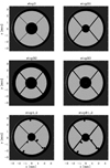 |
Fig. 18. Pupil stop images for the SPHERE visual coronagraph taken with the internal point source and the pupil imaging lens. |
There are two basic types of pupil stops, simple masks which cover only the diffraction rings along the pupil rims for observing modes without pupil stabilization (stop3 and stop1_2) and pupil masks which hide in addition the telescope spiders for pupil stabilized observations (stopB1, stopB2, stopB3 and stopB1_2). Because of the bad actuators of the deformable mirror, special stops with blockers for the scattered light from these actuators located close to the pupil rim or spiders were manufactured (stop1_2 and stopB1_2). Different inner and outer stop diameters allow an optimization for high throughput (stopB1, stop1_2, stopB1_2), for a good rejection of the diffracted light (stopB2), or for an intermediate case (stop3, stopB3). The masks stop1_2 and stopB1_2 were used in 2015 as default masks.
The effect of the stopB1_2 for a coronagraphic image taken with CLC_S_WF is demonstrated in Figs. 19 and 20 for the close binary α Hyi using filter NB_730 in FW0 and the pupil stabilized imaging mode. The panels in Fig. 19 show in (a) the pupil image Φno_stop without stop and in (c) Φ with pupil stop, while panels (b) and (d) show the corresponding coronagraphic images fno_stop and f, respectively, where the faint companion B is located below and slightly left of the center in these pupil-stabilized, non-derotated images. The bottom panels of Fig. 19 show the differences of the two pupil images Φno_stop − Φ and the difference for the corresponding PSFs images c ⋅ fno_stop − f, where the scaling factor c = 0.68 accounts for the reduced off-axis flux transmission because of the geometric attenuation by the pupil stop.
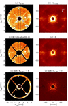 |
Fig. 19. Images of the pupil plane (left) and the center of the focal plane (right) for a coronagraphic observation of α Hyi with the focal plane mask CLC-S-WF without pupil stop (top row) and with pupil stop (middle row). The bottom panels are the differences of the two upper panels. |
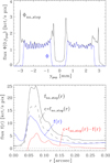 |
Fig. 20. Vertical pupil intensity profiles Φ (top) and mean radial profiles f(r) (bottom) for the coronagraphic observation (CLC_S_WF) of α Hyi without pupil stop (black) and with stopB1_2 (blue). The red curve in the bottom panel shows the diffracted light in the focal plane which are suppressed by the pupil stop. |
The vertical cross section through the pupil and the radial PSF profiles plotted in Fig. 20 allow a more quantitative assessment of the different features in the pupil plane and the focal plane. The profiles Φ(0, y) show clearly the contribution of the extra light in the diffraction rings at y ≈ ±0.4 mm and ±3 mm above the average level of about 1300 ct pix−1. The relative contribution of the diffracted light is about Φdiff/Φno_stop = 5.0%, while the contribution of the 8 brightest maxima caused by bad actuators is Φdead/Φno_stop = 1.5%. In addition there is also scattered light outside the pupil r > 3 mm and inside the central hole r < 0.4 mm which accounts for about Φscatt/Φno_stop = 2.5% of the total light in the pupil.
The pupil stop covers the diffracted light at the inner and outer pupil edges, most of the dead actuator peaks, and the scattered light inside and outside the telescope aperture. Beside this, the stop has a geometric transmission of Tgeom = 72.6% of the telescope aperture. An approximate relation for the ratio of transmitted light with and without pupil stop is therefore

The alignment of the pupil stop in Fig. 19 is offset by about 0.13 mm toward the left and slightly downwards. For this reason the telescope spiders on the upper left and lower right are not hidden by the pupil mask spiders. Fortunately, the misalignment is sufficiently small, so that the special light blockers still attenuate the unfocused light from the dead actuators. The noticed small misalignment is certainly not ideal, but also not devastating because the telescope spiders are not an important flux feature (< 1%) in the pupil.
Important is the attenuation of the diffracted light in the pupil for the reduction of the diffraction rings in the final coronagraphic science image. Because of the diffraction suppression the faint component B of α Hyi is much better visible in the coronagraphic image taken with pupil stop. Figure 20 compares the radial profiles for the coronagraphic images with f(r) and without pupil stop fno_stop(r). This comparison has to consider the reduced effective telescope aperture and therefore throughput c = Tgeom = 0.726 because of the geometric attenuation of the stopB1_2. The difference c ⋅ fno_stop(r)−f(r) (red curve in Fig. 20) illustrates the suppression of the diffracted light from the central star by the pupil stop. The effect is particularly large in the radial range ρ ≈ 0.06″−0.20″. The level of light in the coronagraphic image is reduced by factors ≈0.63 and 0.55 at the diffraction ring peak separation of 76 mas and 115 mas, respectively, and ≈0.71 for the minimum at 94 mas. Thus the effect is very significant near the coronagraphic mask.
The gain in the contrast performance is not only a function of the residual coronagraphic flux f(r), but also on the speckle noise near the coronagraphic mask. It is difficult to give a general “gain value” for a coronagraphic system, because the speckles depend so much on the observing conditions. For the one case investigated here for α Hyi, the gain in S/N for the measurement of the companion at ρ = 0.091″ is thanks to the suppression of the diffracted light by stopB1_2 a factor of ≈1.9 higher than without stop as listed in Table 10 under test A.
4.3. Coronagraphic performance at small inner working angle.
Of great interest is a comparison of the different coronagraphs for the detection and flux measurements of the faint companion to α Hyi separated by 91 mas. Figure 21 shows the innermost region of the images obtained with (a) the small CLC-S-WF mask ( ρ = 46.5 mas), (b) the medium CLC-MT-WF mask ( ρ = 77.5 mas), (c) the four quadrant phase mask 4QPM2, and (d) with non-coronagraphic observations. Apart from the mask, the instrument configuration for (a) and (b) is identical. For the non-coronagraphic image the primary star is offset from the focal plane mask (CLC-S-WF) by 550 mas and a ND2-filter is inserted in FW0 to avoid heavy saturation. These three data sets were taken with the I_PRIM filter for cam1 (shown in Fig. 21) and the R_PRIM filter for cam2. For the 4QPM2 images the N_I filter for cam1 and the cnt820 filter for cam2 are used which match the wavelength of the phase mask.
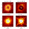 |
Fig. 21. α Hyi A and B observed in the I_PRIM filter with panel a: small and panel b; medium MT classical Lyot coronagraph, panel d: without coronagraph, while (panel c) was taken in the N_I band filter. and the four quadrant phase mask 4QPM2. The circles are flux apertures for component A (center), component B at ρ = 91 mas (black), while (panel a) shows also the concentric comparison apertures. North is up and east to the left. |
In all these images the faint B component can be recognized, at least if its position is known. As illustrated in Fig. 21(a), the flux fB is measured in the black aperture with a radius of r = 7 pixels, subtracting the background level derived from the mean counts in the surrounding pixel ring with 7 < r < 8 pix. This result is then corrected by the mean flux in the eleven white (“empty”) apertures at the same separation to account for a possible systematic effect introduced for example by diffraction rings. The standard deviation for the empty apertures is used as uncertainty σB, and for the signal-to-noise ratio S/N = fB/σB given in Table 10. The flux of B is given as ratio fB/fA, where fA is the flux of the primary measured in the non-coronagraphic PSF, scaled with the transmission of the ND2-filter TND2 = 0.95%, for I_PRIM and 0.73% for R_PRIM.
The measured contrasts fB/fA in Table 10 show a clear trend with wavelength, because the faint companion is redder than the primary star. For a given filter, similar ratios fB/fA are obtained for the different coronagraphs or instrument configurations and the (S/N)B-values give a rough measure of the contrast performance. However, because atmospheric seeing conditions and therefore AO performance are variable one should not give too much value on individual measurements.
Table 10 compares under test B the coronagraphic detection performance of CLC-S-WF, CLC-MT-WF, and 4QPM2. For all three coronagraphs the (S/N)B is about 2.0−2.5 times higher than for non-coronagraphic images taken at the same wavelength. This confirms the results of the coronagraphic test A, which shows that a significant fraction of the diffracted light is suppressed at small separations by the coronagraph.
Overall, the coronagraphic tests B show, that a faint companion at 0.091″ separation with a contrast fB/fA ≈ 0.002 − 0.005, which is hardly or not visible in non-coronagraphic observations, is clearly detected if a small or medium Lyot coronagraph, or a 4QPM is used.
4.4. High contrast observations and image rotation
Field rotation is a very powerful strategy in high contrast imaging to correct for quasi-static instrumental features in the PSF of the central star. With so-called “roll subtraction” of two or several images taken with different sky orientations the stellar light can be significantly reduced and the companion becomes more apparent (Schneider et al. 2003). Even higher contrast levels can be achieved with angular differential imaging which is based on a large number of frames taken with continuous field rotation, where for each image or image section a reference PSF is subtracted, which is derived from appropriately selected frames (Marois et al. 2006; Lafrenière et al. 2007), or a PSF fitting procedure (Amara & Quanz 2012; Soummer et al. 2012).
Figure 22 shows a very simple test for roll subtraction with SPHERE/ZIMPOL, based on three coronagraphic frames of α Hyi taken in field stabilized mode with the different field orientation angles δθ = 0°, 60°, and 120° (see Fig. 22). The individual frames show quite strong variations in the relative companion flux fB/fA and signal-to-noise (S/N)B (Table 10, Test C), which are caused by atmospheric changes and the fact that fA was taken from a non-simultaneous measurement for the fB/fA ratio. Derotating and averaging the frames taken with δθ = 0°, 60°, and 120° does not enhance much the (S/N)B, most likely because the static noise features from the instrument are added to the mean in three different orientations. Nonetheless, the mean flux ratio fB/fA are good flux ratios for the α Hya system in the I_PRIM and R_PRIM band, because these are means based on a total of three minutes of observations.
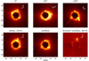 |
Fig. 22. Coronagraphic images of α Hya taken in the R_PRIM filter, the CLC-S-WF coronagraph and with image rotation 0°, 60°, and 120° (upper row). The lower row shows the mean of the derotated images (left), the median of non-derotated image (middle), and the mean of the rotated difference between non-derotated image and non-derotated median (right) as result of a simple roll-angle angular differential imaging procedure. |
Roll-subtraction is more efficient in enhancing the contrast performance than simple averaging. For field-stabilized observations, the telescope pupil rotates and therefore the effects fixed to the telescope, like the spider pattern, are not corrected. However, the orientation of the AO system and the coronagraph as seen by the detector remains unchanged in SPHERE/ZIMPOL because the derotator is located further upstream. Figure 22 shows the median image of the three frames taken with δθ = 0°, 60°, and 120°, which is then subtracted from all three individual frames and the resulting residual frames are derotated and averaged. Of course, the subtraction of a median image from only 3 frames is only a very basic procedure and the derived flux ratios suffer from self-subtraction effects (Table 10, Test C). However, this example shows that the final S/N-ratio is roughly doubled with respect to an individual image and it reveals in coronagraphic images of SPHERE/ZIMPOL quite a lot of fixed instrumental structures from the AO-system and the coronagraph, which can be removed with image rotation.
This kind of simple roll-subtraction can be achieved with only several, for example five exposures taken at different field position angles within a few minutes. Much more telescope time is required for higher contrast observations using the field rotation in pupil stabilized mode or fixed derotator mode, because one needs to stay on target for a time of the order of an hour to achieve a sufficient sky rotation for an efficient ADI data reduction.
5. SPHERE/ZIMPOL imaging polarimetry
ZIMPOL-polarimetry is a powerful differential imaging technique for high contrast observations, because the opposite polarization directions are measured simultaneously and with the same detector pixel, that is through almost the same optical path yielding images that are close to identical for an unpolarized source. Therefore, the PSF of a bright, unpolarized central star, including the variable residual AO speckles, is strongly suppressed in the differential signal, and a weak circumstellar polarization signal may become visible in the polarimetric images.
5.1. Intrinsic polarimetric signal from the sky target
The SPHERE/ZIMPOL polarimetric imaging mode determines the linear polarization of a target at each point in the field of view (α, δ) described by the Stokes parameters,
 (11)
(11)
 (12)
(12)
where the indices of I give the sky orientation for the electric field vector of the photons wave measured from North over East. The polarimetric images Q or U are vector components, unlike the intensity image I, and their signal can contain regions with positive and negative values. Therefore, the measured net signal depends on the spatial resolution of the data, and strong cancelation can occur, if the intrinsic +Q and −Q quadrant pattern from circumstellar scattering is not well resolved (see e.g. Schmid et al. 2006b). A quantitative polarimetric measurement should always consider these cancelation effects because of the limited spatial resolution.
Every polarimetric frame provides also a Stokes I-image or intensity frame which can be reduced and analyzed like “normal” imaging. The intensity is simply the sum of the intensity components, either
 (13)
(13)
 (14)
(14)
For a perfect instrument IQ = IU = I and any deviations from this equality is a spurious measuring effect.
The ZIMPOL IQ- and IU-frames obtained in polarimetric mode contain in principle the same information like the frames taken in imaging mode. The polarimetric IQ and IU have some properties which can be beneficial for certain science applications, like:
-
a lower read-out noise for the slow polarimetry mode which is particularly suitable for faint sources,
-
more accurate absolute and differential (2-channel) photometry, because the photometric throughput depends on instrument polarization effects which are controlled in polarimetric observations. This is an obvious problem for an Nasmyth instrument, where the Al-coated VLT M3 mirror introduces in the ZIMPOL spectral range about 4% of polarization and where channel splitting is done with a polarization beam splitter.
-
the presence of more detector pixel faults, caused by the charge shifting over pixels with non-optimal charge transfer efficiency, requires a more sophisticated observing strategy and data reduction for bad pixel cleaning,
-
no pupil-stabilized polarimetry for angular differential imaging (ADI) – instead there exists a static DROT-mode optimized for polarimetry. This provides a rotating field for ADI, but also the pupil is rotating with a rotation rate different to the field and therefore instrument features fixed to the pupil are less well suppressed,
-
a reduced throughput (≈ − 15%) because of the additional polarimetric components in the beam,
-
the presence of a few additional ghost features caused by the polarimetric components.
The normalized Stokes parameters Q/I and U/I are important parameters for the characterization of astronomical sources, but also for the determination of instrumental polarization effects from the telescope and the instrument. In SPHERE/ZIMPOL the instrumental polarization is to first order field-independent and lower than  as measured with zero polarization calibration stars (see next sections). In many science cases the central star can be a useful zero polarization calibration source for a correction of the instrumental polarization assuming Qstar/I = Ustar/I = 0. This is achieved by applying a re-normalization, ensuring that I0 = I90 and I45 = I135 to the data. If the polarization of the central star is indeed zero then the residual polarization might be produced by a circumstellar polarization component Qcs and Ucs. Such self-calibration procedures were often successfully applied to high contrast imaging polarimetry to disentangle the signal of a circumstellar polarization source from the instrumental polarization (e.g. Quanz et al. 2011; Avenhaus et al. 2014). This procedure corrects also for the interstellar polarization produced by the dust along the line of sight. However, an accurate polarimetric measurement remains an issue for self-calibrated data without a detailed assessment of the instrumental polarization effects.
For a weak circumstellar emission of scattered light it is often much easier to measure the differential polarization signal Qcs and Ucs than the intrinsic intensity Ics. The measured intensity near a bright star is composed of an intrinsic circumstellar component Ics(α, δ) and a dominating and strongly variable component Istar(α, δ, t) from the halo of the central star
 (15)
(15)
Often, there is Ics(α, δ)≪Istar(α, δ) and therefore Ics cannot be determined while the differential polarization Qcs and Ucs can still be measured. Without Ics(α, δ), it is not possible to derive the fractional polarization Qcs(α, δ)/Ics(α, δ) and Ucs(α, δ)/Ics(α, δ). For these cases, one can use the polarized surface brightness contrasts Qcs(α, δ)/Istar and Ucs(α, δ)/Istar which relate the measured circumstellar Stokes signals to the total flux of the central star as measured in a large aperture, for example with a diameter of 3″.
The Stokes fluxes Q and U, and the corresponding fractional Stokes parameters Q/I and U/I or contrast values Q/Istar and U/Istar, are the two components of a vector quantity, where the linearly polarized flux P(α, δ), or the corresponding fractional polarization p(α, δ), is the length of the vector and the polarization position angle θ(α, δ) its orientation (measured from N over E):
 (16)
(16)
 (17)
(17)
The polarized flux P and the polarization angle θ are well defined quantities, if the polarization signal P is significantly larger than the noise. For weak Q or U signals the individual pixel values will have positive or negative signs because of the noise in the data. According to the definition of the polarized flux P in Eq. (16) the Q 2 and U 2 terms count “negative noise values” like positive values and a net polarization results even if the mean Q- or U-signals are zero (e.g. Clarke et al. 1983). Therefore, one should use the individual Stokes Q- and U-values and images for the measurement of a weak polarization signal. The determination of the polarized flux P, the fractional polarization p = P/I, or the polarization contrast Cp = Pcs/Istar needs to take the bias effect of noisy data into account. For centro-symmetric linear polarization patterns, as expected for example for nearly centro-symmetric and optically thin circumstellar scattering, it can be very useful to define radial or azimuthal Stokes parameters with respect to the central object as proxy for the polarized flux, e.g. Qϕ ≈ P, as described in Schmid et al. (2006b).
5.2. Control of the polarimetric signal
ZIMPOL measures according to Sect. 2.2.2 the differential polarimetric signal PZ(x, y)=I⊥(x, y)−I∥(x, y) (Eq. (4)) at the position of the polarization modulator. This signal includes the polarization from the sky target, but also the polarization effects introduced by the telescope and the SPHERE/ZIMPOL instrument. The system concept needs to control the polarization, so that the initial sky target signal can be reconstructed from the measurements taken with different HWP2 orientations i
 (18)
(18)
using appropriate calibrations.
The polarimetric concept of SPHERE/ZIMPOL is complex, because the instrument is fixed to the VLT Nasmyth platform. The strongly inclined M3 mirror of the telescope introduces already at the telescope focus a strong telescope polarization I → Q and polarization cross talks U ↔ V (see Tinbergen 2007). In addition there is an image derotator in SPHERE, which introduces similarly strong polarization effects.
For this reason, SPHERE/ZIMPOL uses an innovative concept which compensates and controls the instrumental polarization of the telescope and instrument with four steps.
-
The M3 mirror of the VLT UT3 telescope has an incidence angle of 45° and an Al-coating which produces in the 500−900 nm range a polarization of about 3−5% and a strong U → V polarization cross talk. This polarization is compensated with the rotatable, achromatic half-wave plate HWP1 and the following first mirror (PTTM) which has also an incidence angle of 45° and a similar Al-coating. HWP1 has an altitude a dependent orientation θHWP1 = a/2 + 45°, which switches the M3 polarization effects into a direction, like for a M3 mirror pointing in zenith direction. The following PTTM mirror acts then like a crossed mirror and compensates the M3 polarization effects to significantly smaller values, for the three components M3-HWP1-PTTM (Joos 2007). Figure 23 shows for the unpolarized star ϵ Eri the residual fractional telescope polarization qtel = Qtel/I and utel = Utel/I after M3-HWP1-PTTM. Hereafter, we call this also the telescope polarization because it is fixed to the telescope and therefore changes with the parallactic angle θpara. The telescope polarization can be corrected with calibrations of zero polarization standard stars (see Sect. 5.3.1). A polarization compensation with a crossed-mirror was already described by Cox (1976) for an instrument fixed to the telescope tube, while Martinez Pillet & Sanchez Almeida (1991) included also a rotating half-wave plate for narrow-band applications with a Coudé-focus instrument for solar physics. SPHERE/ZIMPOL introduces now this approach for broad-band, high contrast imaging polarimetry for an Nasmyth instrument at a stellar telescope (see also Tinbergen 2007).

Fig. 23. Residual telescope polarization qtel = Qtel/I and utel = Utel/I as function of parallactic angle for the unpolarized star ϵ Eri in the VBB filter. Also shown are the measurements q +, q −, u +, and u − of a polarimetric cycle, which include instrument polarization component ±pSZ for the P2-mode and a field position angle offset of 60°.
-
The fractional Stokes parameters for the instrument polarization of SPHERE/ZIMPOL qSZ and uSZ includes all components after the PTTM in CPI (Fig. 1) up to the ZIMPOL polarization modulator. This polarization is compensated with a measuring procedure, where HWP2 is used as Q +, Q −, or U +, U − polarization switch by applying to the HWP2 position angle an offset cycle of 0° and 45°, or 22.5° and 67.5°, respectively. The 45° offset, or Q − switch, reverses the sign of the target and telescope polarization Q + qtelI, with respect to the Q + offset position, while the polarization effects introduced by the following components qSZI and uSZI are unchanged. Subtracting the Q − from the Q + measurement cancels qSZ after HWP2 and only Q + qtelI remains
![Mathematical equation: $$ \begin{aligned} Q^+ - Q^-&= [(Q+ q_{\rm tel} I) + q_{\rm SZ}I] - [-(Q + q_{\rm tel}I) + q_{\rm SZ}I]\nonumber \\&= 2\, (Q + q_{\rm tel}I). \nonumber \\ \end{aligned} $$](/articles/aa/full_html/2018/11/aa33620-18/aa33620-18-eq30.gif) (19)
(19)and similar for the U polarization component. The polarization switch is a well known technique to compensate instrumental polarization to first order (e.g. Appenzeller 1968; Kemp & Barbour 1981; Scarrott et al. 1983) and Fig. 23 gives an example for SPHERE/ZIMPOL for the unpolarized star ϵ Eri with an intrinsic polarization Q/I and U/I < 0.001 (Tinbergen 1979). It is important to locate the HWP-switch as early as possible in the beam for keeping the non-compensated instrumental polarization qtel and utel introduced in front of the switch simple and easy to determine.
-
The derotator DROT in SPHERE, a three mirror system with inclinations angles of 55°, 10°, and 55°, is a very critical component for polarimetric measurements because it introduces an instrument polarization (diattenuation) I → Q of m21 ≈ 0.03, and strongly wavelength dependent polarization cross talks U ↔ V, which can be larger than |m34|> 0.5. To minimize the cross talk effects the linear polarization direction to be measured by ZIMPOL is rotated by HWP2 into the I⊥ and I∥ orientation θDROT. This requires, that the HWP2 tracking law considers the rotation of e.g. the I0 sky orientation, compensates at the same time for the rotation effect of HWP1, and rotates the I0 direction into the I⊥ orientation of DROT depending on the derotator law. DROT can either be in a fixed orientation for P1-mode, θDROT = 90° or it moves like θDROT = 0.5(alt − θpara) to stabilize the image on the detector in P2-mode. In these relation one must consider the 180° angle periodicity of θDROT for the image orientation.
-
The derotator polarization of about pDROT ≈ 3% is corrected with the polarization compensator PCOMP, an uncoated, co-rotating, inclined glass plate in ZIMPOL. This plate deflects more of the I⊥-component than the I∥-component, so that I⊥ − I∥ is reduced in the transmitted beam (Sect. 2.2.3). For an inclination of 25°, the current value used for PCOMP, the derotator polarization and other minor contributions from other components are reduced to about 0.3%.
5.3. Calibrations for the polarimetric measurements
The polarimetric measuring strategy includes four calibration steps:
-
c1 is the correction for the ZIMPOL modulation-demodulation efficiency ϵmod as described in Sect. 2.3.3 (Table 5). For the determination of the fractional polarization in a large aperture also the frame transfer effect or ϵft (Eq. (6)) needs to be considered. The calibration factors ϵmod are obtained with a fully polarized illumination using the internal flat field source and the polarizer in FW0.
-
c2 is the subtraction of the telescope polarization which depends on pointing direction and filter. The telescope polarization ptel and θtel is determined with zero-polarization standard star calibrations.
-
c3 is a small correction for the polarization efficiency loss of the telescope mirrors M1 and M2 and that part (residual polarization cross talk) of the M3-HWP1-PTTM configuration, which is not included in the modulation-demodulation efficiency calibration ϵmod. The effect is small with a correction factor close to one, which can be checked with high-polarization standard star calibrations.
-
c4 is a position angle offset correction for the effective HWP2 plate orientation to adjust the measured Q, U parameters to the North direction on sky. This polarization angle offset δSZ depends slightly on wavelengths and is also calibrated with the high-polarization standard stars.
The calibrations c1 and c2 are very important for all quantitative polarimetric measurements. The corrections or adjustments c3 for ϵopt and c4 for δSZ are only relevant for high signal-to-noise polarimetry S/N = p/Δp ≳ 20. However, all calibrations are essential for checking the proper working of the instrument and one should be alarmed if unexpected calibration results are obtained.
5.3.1. Calibration of the telescope polarization
The “residual” telescope polarization is regularly measured with zero-polarization standard stars (p0pol ≪ 0.1%), as part of the ESO SPHERE instrument calibration plan. We use bright, nearby, single solar type stars, preferentially from the lists of Serkowski et al. (1974) or Tinbergen (1979). These measurements consist typically of one full polarimetric cycle for each of the three filters V, N_R, and N_I in FW1 and FW2. Often ND-filters are used in FW0 in order to avoid saturation. All these calibration data are available in the ESO archive.
For the analysis the measurements are bias subtracted and corrected for the modulation-demodulation efficiencies ϵmod and the frame transfer effect ϵft. Integrated fluxes Q, U and IQ, IU are determined for synthetic apertures and fractional telescope polarization parameters qtel = Q/IQ, utel = U/IU, ptel and the position angle θtel is calculated.
We have analyzed all useful zero-polarization standard star calibrations from 2015, which include 17 measurements for each of the three filters V, N_R, and N_I. The derived telescope polarization values are in the range ptel = 0.4 − 0.6% with a scatter of only σp ≈ 0.04% for a given filter. As shown in Fig. 24 the polarization position angle θtel is proportional to the parallactic angle θpara with a wavelength dependent offset δtel(λc)
 (20)
(20)
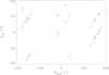 |
Fig. 24. Telescope polarization angle θtel as function of the parallactic angle for zero-polarization standard stars measured in the filters V (green), N_R (red), and N_I (black) with dotted lines for the best fits according to Eq. (20). Blue diamonds are the VBB-filter data from Fig. 23. |
where one must consider the 180° polarization angle periodicity. Table 11 lists for the zero-polarization standard stars the mean polarization ptel and standard deviation σp, and the mean position angle offset δ and σθ from the best fit (Eq. (20)) also plotted in Fig. 24. The correlation between θtel and θpara is expected because the compensation of the M3 mirror polarization with the HWP1 – PTTM combination yields residuals which are to first order fixed to the telescope pupil. This effect is also nicely seen in Fig. 23 for the long data series of the unpolarized star ϵ Eri taken in Nov. 2016.
Table 11 gives additional measurements for the wavelength dependence of ptel(λc), δtel(λc) based on multifilter data of ζ Tuc (HR 77) taken during SPHERE commissioning in Oct. 2014. The color dependence of ptel and δtel can be explained by differences in the M3 and PTTM mirror coatings and some deviations of HWP1 from a perfect, broad-band half wave plate. The strong rotation of δtel in the I-band is probably related to the well known reflectivity minimum of Al-coatings in this wavelength range. One might expect a slow temporal evolution of the telescope polarization because of the aging of the mirror coatings and perhaps a sudden change associated with the M1 and M3 telescope mirror re-coating, which took place in April 2017.
Measurements of the fractional polarization Qc1/I and Uc1/I of standard stars, can now be corrected for the telescope polarization according to
 (21)
(21)
 (22)
(22)
The parameters ptel and δtel from Table 11 can be used for all observations from 2015 and possibly also for later observations. One should notice that the corrected values Qc1/I and Uc1/I for the standard star polarization parameters derived in large apertures must use the factors ϵmodϵft including the frame transfer smearing effect (Table 5).
5.3.2. Calibration of the polarization angle and efficiency
Also high-polarization standard star measurements are taken regularly in the V, N_R, and N_I filter as part of the ZIMPOL calibration plan. These data provide an independent test for the corrections c1 and c2. For our analysis all well illuminated high polarization standard star calibrations from 2015 are included. The measurements and data reduction of high-polarization stars are identical to the zero-polarization standards described above.
Table 12 lists the obtained polarization values for the standard stars, after applying corrections c1 and c2, and compares them to literature values. Figure 25 shows the data for the N_R-filter in the Q/I − U/I-plane with black symbols for c1 corrected values, and red symbols with the additional telescope correction c2 applied. The literature values are given in blue. Also shown are the 17 N_R zero-polarization standard star data from the previous section located on a ring with radius r ≈ 0.5%, and the telescope corrected red points are clustered near the zero point with a small scatter of σp = 0.12%. A similar pattern of black points surrounding the telescope corrected red values is also present for the high-polarization standard HD 183143.
Measured and corrected polarization pc [%] and θc [°] of high-polarization standard stars and comparisons with literature values pℓ, θℓ.
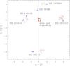 |
Fig. 25. Polarization of high polarization standard stars for the N_R filter: black symbols give efficiency or c1 corrected values while red symbols are also corrected for the telescope polarization (c2-correction). For individual targets, either plus-signs or diamonds are used in order to avoid confusion. Corresponding literature values are plotted as blue squares with error bars. Also included are the zero-polarization standard stars from the previous subsection. |
The derived polarizations (red symbols in Fig. 25) for the high-polarization stars are slightly offset or rotated in counter-clockwise direction when compared to the literature values of high polarization stars. This is summarized in Table 12, which compares for all three filter V, N_R and N_I the ratio pc/pl between the measured polarization pc and the literature value pℓ, and the difference Δθc − ℓ = θc − θℓ between the derived polarization angle θc and the corresponding literature value θℓ. The measurements were first corrected for the modulation efficiency and frame transfer smearing ϵmodϵft (Eq. (7)) and the telescope polarization (Eqs. (21) and (22)). The bottom rows give as final result for each filter the average ratio ⟨pc/pℓ⟩ and the average angle difference ⟨Δθc − ℓ⟩ for the ZIMPOL V, N_R, and N_I filters. The average ratios ⟨pc/pℓ⟩ are compatible with 1, while ⟨Δθc − ℓ⟩ indicates at least for the N_R and N_I filters significant polarization angle offsets δSZ for SPHERE/ZIMPOL.
The results of the high polarization standard star measurements should be considered as preliminary values. For HD 183143 it is clearly visible, that the scatter of σp = 0.52% for the red corrected points in Fig. 25 is significantly larger than the σp = 0.12% for the zero-polarization standard stars.
Several effects contribute to this enhanced scatter in the high polarization standard star data. First, there could be instrumental cross talk effects Q → U, V or U → Q, V, which may depend on instrument configuration, and become apparent for objects like HD 183143 with a high linear polarization pstar ≈ 5%. Because these cross talks scale with p, they are much smaller for the zero-polarization standard stars. Second, the standard star measurements could be improved. They are not taken in a homogeneous way and would require a study on its own to minimize systematic measuring effects, e.g. differences between strongly and weakly illuminated data. Third, the polarization of the high polarization standard stars could be variable, and HD 183143 is apparently such a case (Hsu & Breger 1982). Achieving a smaller uncertainty Δp < 0.5% in absolute polarimetric measurements of high polarization target with ZIMPOL is certainly possible but requires but requires an extensive analysis of data from well suited calibration targets which is beyond the scope of this paper.
We summarize here briefly the status of bright high polarization standard stars suitable for the calibration of ZIMPOL observations. Only the more northern δ > −30° objects HD 147084 and HD 154445 were established as good calibration stars by Hsu & Breger (1982), and their values are in good agreement Δp ≈ ±0.1%, Δθ ≈ ±1° with Bailey & Hough (1982), and Serkowski et al. (1975). As mentioned above HD 183143 is known to show some polarimetric variability (Hsu & Breger 1982) and the same is true for several other high polarization standard stars (Bastien et al. 1988, 2007). The situation is even worse for the southern Milky Way δ < −30°, because there exist essentially no well established bright high polarization standard stars suitable for SPHERE/ZIMPOL. The used objects HD 79186, HD 98143, and HD 111613 have been measured polarimetrically (Serkowski et al. 1975; Whittet et al. 1992), but the accuracy of the published values is unclear and the absence or the level of polarimetric variability has not been investigated.
5.3.3. Recommended polarimetric correction formulae
The full correction of the measured Q and U signals of a science target requires two steps: first the corrections c1 for the modulation efficiency ϵmod, c2 for the telescope polarization, and c3 for a small efficiency loss because of the optical components:
 (23)
(23)
 (24)
(24)
Note, that the polarization flux parameters Q and U are not affected by the intensity dilution during the frame transfer, and therefore ϵft is not considered.
In a second step the obtained values Qc3 and Uc3 are then rotated “polarimetrically” to correct for the polarization angle offset of a few degrees,
 (25)
(25)
 (26)
(26)
Most important are the corrections c1 and c2 for the modulation efficiency ϵmod = 0.75 − 0.91, which depends on instrument parameters, and the additive telescope polarization Δ(Q/I),Δ(U/I)≈ − 0.6 to +0.6%. The corresponding parameters ϵmod are given in Table 5 and ptel(λc) and δ(λc) for the telescope polarization are listed in Table 11. The corrections c3 and c4 for the optical efficiency ϵopt and the position angle offset δSZ are only important for strongly polarized objects Q/I, U/I ≳ 2% which can be measured with a high polarimetric signal-to-noise S/N = Δp/p ≳ 20. The value ϵopt and δSZ(λ) have not been determined yet with high precision and we recommend a value of  and δSZ(λ)=⟨Δθc − ℓ⟩ according to Table 12.
We think that SPHERE/ZIMPOL provides a substantial progress in quantitative polarimetry for AO assisted, high resolution observations because the instrument polarization effects are well controlled and calibrated with accurate standard star measurements. Therefore, quantitative measurements can also be obtained for weak, non-axisymmetric and other demanding targets. Infrard instruments, like SPHERE/IRDIS (Langlois et al. 2014; van Holstein et al. 2010) and GPI (Perrin et al. 2015) provide also calibrated polarization measurements so that the diagnostic potential of multi-wavelength polarimetry can be exploited.
5.4. Differential polarimetric beam shifts
An important requirement for the performance of a high-contrast, differential polarimetric imager are small aberrations between the measured I⊥ and I∥ images. In ZIMPOL, these two polarization modes are registered with the same detector pixels to minimize optical aberrations. Small differential beam shifts between I⊥ and I∥ can be produced by non-perfect half-wave plates and this was considered in the ZIMPOL design. During instrument tests small beam shifts from the modulator assembly were measured, but they were less than 0.1 pixels (< 0.4 mas) and considered to be acceptable (see Roelfsema et al. 2010).
Unfortunately, we detected after the integration of ZIMPOL into SPHERE a substantially larger and unexpected beam shifts of up to 0.3 pixels (or ≈1 mas) between I⊥ and I∥ caused by the inclined mirrors in CPI. These differential polarimetric beam shifts are apparent in Q or U images as systematic positive and negative features on opposite sides of a stellar PSF (see Fig. 26) and this affects the speckle suppression capabilities of the polarimetric mode. This subsection outlines the origin of this effect, illustrates the impact, and gives a recipe for correcting the effect.
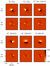 |
Fig. 26. Observed polarimetric beamshift for a stellar PSF of α Cen B taken in June 2016 with the VBB and ND4 filters: The first row shows two consecutive polarization frames (Io − Ie)0 and (Io − Ie)Π taken with opposite, zero and pi demodulation phase shifts and the resulting, charge-trap corrected, Q+-frame. The third row illustrates the beamshift for the derotated Q+-, Q−-, and the final “science” Q-image. The second and bottom rows show the same but with the beamshifts corrected between the odd-row Io and even-row Ie sub-frames. |
5.4.1. Polarization aberrations from inclined mirrors
Extensive SPHERE/ZIMPOL testing showed that the main contributions to the differential polarimetric beam shifts are caused by the strongly inclined mirrors M3 of the telescope, the 45° pupil tip-tilt mirror (PTTM), and the image derotator mirrors, while the half wave plates are at most minor contributers.
PSF shifts between I⊥ and I∥ are introduced by inclined metallic mirrors because the Fresnel coefficients for the phase shift are different for I⊥ and I∥ as described by Breckinridge et al. (2015) in a comprehensive analysis of polarimetric aberrations of telescopes. The same type of beam shifts causing deviations from the law of geometric optics on sub-wavelength scales are also known in optics as Goos-Hähnchen (GH) and Imbert-Federov shifts (e.g. Aiello et al. 2009; Bliokh & Aiello 2013). These shifts are not well known for astronomical instruments, because the spatial resolution or/and polarimetric sensitivity of previous instruments did not achieve the SPHERE/ZIMPOL performance. Therefore, we describe here the dominant effect and provide a simple calculation for the expected PSF shift.
A beamshift between the two polarization components I⊥ and I∥ reflected from an inclined surface was first described by Goos & Hänchen (1947). The reflected I⊥ and I∥ components are shifted as expected for slightly offset “effective” mirror surfaces for the I⊥ and I∥ components. This is illustrated in Fig. 27 with a simplified ray model for the principal beam (solid black, blue and red line with arrows) for two hugely exaggerated offsets for the “effective” mirror surfaces. The induced beam displacements are attributed to the phase shifts ϕ introduced in the reflection, which depend on inclination angle θ. As shown by Artmann (1948) with an angular spectrum decomposition and interference for a spatially limited beam, the incidence angles of the incoming wave sections vary around the incidence angle θ0 and therefore the waves receive an angle dependent phase shift in the reflection. This explains a spatial Goos-Hähnchen shift Δ, which is proportional to the phase shift gradient dϕ/dθ
 (27)
(27)
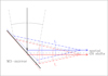 |
Fig. 27. Schematic and simplified illustration of the polarimetric beam shift effects for the M3 Nasmyth mirror. The incoming beam and the expected reflection according to geometric optics are plotted in black. The beam and wavefront displacements for I⊥ and I∥ caused by the phase shifts, with the corresponding “effective” mirror surface location and tilts, are hugely exaggerated and drawn in red and blue respectively. |
For metallic mirrors, positive and negative shifts are introduced for I⊥ and I∥, respectively, because dϕ⊥/dθ and dϕ∥/dθ have opposite signs. There exists also a transverse beam-shift, called spatial Imbert-Fedorov shift (e.g. Bliokh & Aiello 2013), which is also of some importance. The so-called angular shifts, another type of the beam-shifts caused by the angle dependent reflectivity of metallic mirrors, are not relevant for the image position in a focussed beam. It is beyond the scope of this paper to describe here in detail all these effects.
The beam shift can also be explained for a “macroscopic” view of the converging beam of a Nasmyth telescope with an inclined mirror M3 as sketched for the propagation of the wavefronts in Fig. 27, and described in more detail in Breckinridge et al. (2015). In this case, the angles of incidence θ on M3 are different, 45 ° +ϵ and 45 ° −ϵ, for the “left” and “right” sections of the incoming spherical wave fronts in Fig. 27. Consequently, also the phase shift introduced by the reflection is different ϕ(45 ° +ϵ) and ϕ(45 ° −ϵ), so that the interfering spherical wave sections converge along a slightly different angle, when compared to the angle predicted by geometric optics. When neglecting higher order terms, then the estimated focal point shift is about
 (28)
(28)
where F#=f/D is the F-ratio for the converging or diverging beam, and 1/F# the corresponding angular spread for the focused beam. Because the phase shifts gradients dϕ/dθ are different and have even different signs for I⊥ and I∥ for metallic surfaces also positive and negative focal point shifts Θ⊥ and Θ∥ result (Fig. 27). The focal point shifts are proportional to the inverse of the focal length f and therefore the focus displacement expressed in nm in the focal plane does not depend on the telescope size and is just given (to first order) by the phase shift gradient of the mirror coating for the incidence angle θ0
This is the same result as in Eq. (27), because both, a narrow beam and a macroscopic telescope beam are made of an angular spectrum of plane-parallel wavefronts impinging onto an inclined mirror.
The PSF-shifts Δ⊥, ∥ do not depend on the F-ratio, the focal lengths, or the aperture diameter of the focussed beam, but only on θ0 and the mirror surface. For an Al-mirror and λ = 800 nm the phase shift gradients is in units of wavelength per radian
Multiplication with λ/2π yields then the PSF-shifts 19.2 nm and −38.1 nm in the focal plane, respectively, and the differential PSF shift of
For a telescope with the focal length of the VLT (f = 120 m) this differential PSF shift in the focal plane corresponding to an angle shift of Θ⊥ − Θ∥ = 0.101 mas on sky. The derived shift of 57.3 nm agrees with the result of Breckinridge et al. (2015, Table 2), who obtained for the same λ, θ0 and mirror surface a focal point shift of Θ⊥ − Θ∥ = 0.625 mas (=3.15 × 10⁻⁹ rad) for a telescope with f = 19.2 m. This is essentially the same shift Δ⊥ − Δ∥ = 60.5 nm as calculated for the VLT, considering that the used dϕ⊥, ∥/dθ-values used by us could be slightly different.
The same principles for polarimetric beam shifts apply for all inclined mirror in a converging or diverging beam. This are the Al-coated M3 mirror of the telescope, the Al-coated 45° pupil tip-tilt mirror (PTTM), and the image derotator mirrors. The beam-shift introduced by the PTTM is essentially the same as for M3, except for the different mirror orientation. Our measurements show that the derotator is the dominant component for the beam shift in the I- and R-band range, while the shift in the V-band is comparable to the M3 mirror. The strong effect from the derotator is not surprising, because it consists of three mirrors, two 55°-mirrors and one 20°-mirror and the shifts of the two 55°-mirrors add up. They have overcoated silver surfaces and the strong wavelength dependence for the beam shift is probably caused by this type of reflecting surface, for which we do not know the dϕ/dθ phase shift properties.
5.4.2. Correction of the polarimetric beam shift
The SPHERE/ZIMPOL beam shifts are the results of a complex combination of several contributing components, mainly the inclined M3 mirror of the VLT, the 45° PTTM mirror, and the three mirrors in the image derotator. Moreover, the half wave plates HWP1, HWP2 and HWPZ rotate the polarization angle of the shifted components at different locations along the light paths. Several of these components rotate during the observations and therefore each exposure requires an “individual” correction which is only valid for a given sky position and instrument configuration. In particular, the beam shifts for the four exposures of a polarimetric cycle Q +, Q −, U + and U − are all different (see Q + and Q − in Fig. 26). Another significant complication is that the beamshift from the derotator is strongly wavelength dependent with a large, ≈1 mas shift, in the I-band, about 0.5 mas in the R-band and less in the V-band. Because of this complexity, there exists up to now no instrument model for the correction of the differential beam shifts.
However, a beamshift correction can be applied to the science data, if the offset between the science images in the odd-row and even-row subframes Io and Ie can be determined, so that the two frames can be accurately aligned before the polarimetric combination of the frames is carried out (see Fig. 26).
It is more difficult to recenter frames without well defined intensity peaks, e.g. frames with low Strehl ratio, with saturated PSF, or coronagraphic images. For these cases, one can use beamshift corrections derived from short polarimetric cycles of well defined stellar PSFs, taken with the same (or similar) filter, the same polarimetric configuration and telescope orientation. Because the beamshift changes only slowly with parallactic angle and altitude, one can take such beam shift calibrations just before or/and after the science observation, using the PSFs of the same star, or another star with similar pointing directions (parallactic angle and altitude) |Δp| and |Δa|≲5°.
An example for a beamshift correction for a coronagraphic image is shown in Fig. 28, where residuals in the uncorrected differential polarization image is at the level of up to ≈1% in Q/I or U/I near the coronagraphic mask. These data are corrected with the non-coronagraphic PSF measurements of the same star (Fig. 26) taken 10 min later. For this, the star was just offset from the coronagraphic mask and observed with a short integration and a ND-filter. This calibration reduces the residuals in the polarimetric image significantly, for example the standard deviation in the box at the bottom of the frames in Fig. 28 is 9.3 ct in the uncorrected frame and 4.4 ct in the corrected frame.
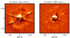 |
Fig. 28. Beam shift effect for α Cen B in the VBB filter for a coronagraphic (CLC-MT-WF) Stokes Q frame (left) and the beam shift corrected frame (right) for essentially the same instrument configuration as the stellar PSF in Fig. 26. The arrow in the left panel points to the PSF peak transmitted through the mask. PSF residual features are marked in the left panel with “t” and “s” according to Fig. 8. In the right panel the arrow points to one of several spots from the camera, which show up because of the applied beam-shift correction. The squares at the bottom mark the area for the reported σ(Q). |
The residual noise is not completely removed by the beam shift correction as can be seen for the strong “s” speckles. The positive/negative ring feature at the edge of the coronagraphic focal plane stop is even enhanced and new spurious positive/negative spots are introduced, as indicated by the arrow in the right panel of Fig. 28. These are intensity features originating from components located after the inclined mirrors. For example, the coronagraph, the deformable mirror, poorly corrected bad pixels, or dust on the micro-lens array of the ZIMPOL detector introduce spurious positive/negative polarimetric signals if a beam-shift correction is applied. Some of these new problems can be solved with detector dithering, but it is still unclear how some of these spurious features can be removed again.
The beamshift can also be measured in high quality coronagraphic images, if the focal plane mask CLC-MT-WF is used. This mask is by design slightly transparent and therefore the same polarization pattern is visible in Fig. 28 (left) for the attenuated star marked with an arrow, as for the stellar PSF shown in Fig. 26 (Q, derot, no.corr). Beamshift corrections based on the transmitted PSF using the CLC-MT-WF masks give good results, if the Strehl ratio for the observations is high and if the star is well centered on the mask. Of course, frame selection is important because a few good frames are sufficient to define the beamshift correction for many exposures of the same target taken before and afterwards.
5.5. Polarized PSF
The quality of the ZIMPOL polarimetric imaging can be assessed with an unpolarized or polarized stellar PSF without circumstellar emission. Such an object should show over the whole image plane a constant fractional polarization. Figure 29 shows the Stokes fluxes Q and U for the V-band of HD 183143 from the same observations used for the characterization of the intensity PSF in Fig. 8. The PSF in Q is just a faint replica of the intensity PSF, with central PSF peak, and speckle ring because the star has a high interstellar Q/I-polarization of about 5%. In U, only a weak negative peak is visible because of the small U/I ≈ −0.5% telescope polarization. These polarimetric PSFs are corrected for the beam-shift effect and therefore they show no positive/negative central features for r < 20 pix. Outside r > 20 pix, no difference is visible between beam-shift corrected and not corrected profiles. The displayed PSFs were also not polarimetrically calibrated, because this has no impact on the polarization structure of the PSF.
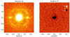 |
Fig. 29. Stokes Q and U images for the V-band filter of the PSF standard HD 183143. These are the polarization images corresponding to the intensity PSF shown in Fig. 8. |
Figure 30 shows the corresponding mean radial Q(r) and the azimuthal profile Q(ϕ, 80) for r = 80 pix through the speckle ring and the same for Stokes U. The lower panels show the corresponding fractional polarization signal, which are essentially constant in the radial and azimuthal profiles without instrumental structures in Q(x, y)/I(x, y) and Q(x, y)/I(x, y) despite the large dynamic range with > 3000 ct pix−1 for the PSF peak and only a few counts per pix and frame further out.
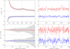 |
Fig. 30. HD 183143 mean radial V-band profiles (left) for the Stokes flux Q(r) and U(r) (top) and the fractional polarization Q(r)/I(r) and U(r)/I(r) (bottom) and the corresponding azimuthal profiles Q(80, ϕ), U(80, ϕ), and Q(80, ϕ)/I(80, ϕ), U(80, ϕ)/I(80, ϕ) (left). The U-data are shifted downwards in for better visibility and the dashed lines indicate the offset. |
This polarimetric fidelity is a particular advantage of the ZIMPOL technique which registers the opposite polarization modes I⊥ and I∥ with the same pixels. The differential polarimetric signal is therefore essentially independent of the exact flatfielding factors a ff
or bias level subtraction values c bias
because the flat-fielding factors  or the bias levels are
  are very close to identical for the two modes. This beneficial property of ZIMPOL is very useful for the analysis of polarization signals from circumstellar sources.
5.6. R Aqr: an example for circumstellar polarization measurements
We used R Aqr as test source for polarimetric imaging during the SPHERE/ZIMPOL commissioning. This object is bright, mI = 4.4m at the time of our observations, and it showed in previous studies with aperture polarimetry strong, and highly variable, linear polarization (e.g. Serkowski & Shawl 2001; Joshi et al. 2012; Aspin et al. 1985). R Aqr is a nearby d = 220 pc symbiotic binary with a Mira variable undergoing heavy mass loss and binary interactions (Schmid et al. 2017, and references therein).
Polarimetric data for R Aqr were taken in many different filters (Schmid et al. 2017), but we focus here on the I-band data taken obtained three different instrument modes:
-
(i)
in fast modulation using the 20 nm narrow-band Cnt820 filter for the PSF peak (hereafter called “nb”-image),
-
(ii)
fast polarimetry in the 150 nm wide broad-band I_PRIM filter where the PSF peak saturated (“sat”-image), and
-
(iii)
deep I_PRIM, slow-modulation polarimetry in coronagraphic mode (“coro”-image) for the “outer” regions.
Polarimetric test data for R Aqr from 2014-10-11 used in this work.
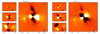 |
Fig. 31. R Aqr I-band Stokes Q (left) and U (right) signal measured for the unsaturated PSF in the narrow-band (nb) Cnt820 filter (upper left), for the saturated broad band I_PRIM filter (middle left), and deep coronagraphic observations for the I_PRIM filter and slow polarimetry mode (lower left and large frame). The cut for the count profiles of Fig. 33 is shown in the large Q-frame. Units are in pixels of 3.6 mas. |
5.6.1. Data reduction
The data were first reduced in a standard way, with an overscan bias subtraction, flatfielding, polarimetric signal extraction and combination. Already these basic steps allow a qualitative analysis of all extended polarization features described below.
In a second step, the reduction was rerun, but with applying a polarimetric beam shift correction before the combination of the polarization frames. The beam shift correction was derived from the unsaturated “nb”-data and also applied to the saturated and coronagraphic I_PRIM filter data. Applying the beam shift correction reveals also a Q- and U-quadrant pattern for the PSF-peak described below, and it reduces spurious polarization residuals at the position of strong speckles.
For an accurate quantitative analysis we correct our data with an image rotation of θ0 = 2° in clockwise direction to account for the astrometric offset from the North direction according to Eq. (2). Then we apply the polarimetric calibrations, deriving first Qc1, Uc1 (Eq. (7)) using the modulation-demodulation efficiencies ϵmod (Table 5), the corrections for the telescope polarization ptel = 0.4%, δtel = 68° from Table 12, which yield for the parallactic angle of the observations (θpara ≈ −114° to −122°) roughly Qc3/I ≈ Qc1/I and Uc3/I ≈ Uc1/I + 0.004 (Eqs. (23) and (24) with ϵopt = 1). As last step we apply a polarization angle offset correction of 6° according to Eqs. (25) and (26). Both, the astrometric correction of 2° and the polarimetric correction of 6° rotate the polarimetric Q- and U-quadrant pattern in clockwise directions so that the slightly tilted patterns from the basic reduction get an orientation which is essentially undistinguishible from the expected up-down/left-right Q-pattern and the corresponding diagonal ±45° U-pattern shown in Fig. 31.
Despite all these corrections, there remain ambiguities in the measured circumstellar polarization of R Aqr because of two effects. The limited resolution produces polarimetric cancellation between the +Q and −Q or the +U and −U regions (see e.g. Schmid et al. 2006b), and the unresolved emission of the star is also intrinsically polarized and contributes to the measured polarization signal as can be inferred from the available multi-wavelength polarimetry taken during the same night. A more detailed analysis would be required to disentangle the intrinsic polarization of the central star from the circumstellar polarization signal. This is of much scientific interest, but must be deferred to a future paper focussing on the mass loss of R Aqr. The scope of this section are the measuring capabilities of SPHERE/ZIMPOL for high performance polarimetry and therefore we just analyze the calibrated measurements.
All data are count normalized ctn6 as in previous sections by setting the total counts of the star within an aperture diameter of 3″ to 106 counts. For the saturated and coronagraphic images, where the PSF peak counts are not available, the halo-flux was adjusted to the normalized, unsaturated “nb”-image for r in the range 100 pix < r < 250 pix. This procedure assumes, that the PSF halo flux remained unchanged and provides a good relative calibration for the three images.
5.6.2. Description of the Stokes Q and U images
The polarimetric data show the typical Stokes Q and Stokes U quadrant pattern of a circumstellar scattering region. The distribution of the scattering dust is a spherical and clumpy causing geometric features in Q and U which deviate clearly from a symmetric, smooth quadrant structure.
Polarization of the PSF peak. The “nb”-images for Q and U in Fig. 31 show the polarization in the PSF peak of the mira variable. Clear Q and U quadrant patterns are visible within r ≲ 15 pix with maxima and minima located at a separation of about r ≈ 5 pixels (18 mas or ≈3.6 AU) from the intensity peak center.
This polarization originates from scatterings in immediate surroundings of the central star. For an unresolved, strictly centro-symmetric scattering case the +Q, − Q or +U, −U components would just cancel, and such a zero is indeed seen in the center. The radius of R Aqr measured by interferometry is about 7–8 mas (e.g. Ragland et al. 2008) or about 2 pixels, thus the peak intensities in the Q and U parameters originates from within 1 − 3 stellar radii. The measurements at small separations depend strongly on the self-cancellation because the intrinsic positive and negative regions of +Q, − Q or +U, −U overlap substantially when convolved with the instrument PSF. Therefore, the fractional polarization inside 5 pix reaches extreme values of only Q/I, U/I ≈ ±0.25%, lower than ≈ ± 1.0% in the surrounding anulii r = 5 − 10 pix, or ≈ ± 1.5% for r = 10 − 30 pix. The intrinsic value for this circumstellar polarization is certainly much larger, but hard to quantify without a detailed simulations of the signal convolution with the instrument PSF.
Polarimetry for 0.03″< ρ ≲ 0.20″. The “sat”-images taken with the 150 nm broad-band filter I_PRIM yielded about four times higher photon counts (for the same exposure time) than the “nb”-image, roughly as expected considering the larger filter width but also the much lower stellar flux in the 750−800 nm region. Several pixels in the PSF peak are saturated and it is difficult to measure the beamshift. Therefore we applied the same beamshift correction as for the unsaturated “nb”-image.
The “sat”-images are ideal for polarimetric measurements of the separation range 30 mas < ρ< 200 mas filling the gap between the saturated peak and the inner working angle of the coronagraphic data. In the “sat”-data of R Aqr (Fig. 31), the polarized intensity Q from the circumstellar dust scattering is stronger on the East-side of the Mira variable than on the West side, most likely because of the hot companion located 45 mas to the West of the mira (Schmid et al. 2017).
Sensitive polarimetric observations in the radial range 30 mas < ρ< 200 mas are demanding because of the huge intensity gradient near the PSF peak with a flux ratio f(0)/f( ρ) ≈ 1000 for ρ = 0.20″ (55 pix). Photon noise limited observations are achievable for the separation range ρ ≈ 0.07″−0.20″ with exposures where the PSF-peak is just at the saturation limit or in saturation by a factor of a few. For lower illumination the read-out noise can dominate already around 0.1″. For strong saturation of more than a factor of > 5 the charges start to “bleed” into neighboring pixels mainly along the detector column direction and this affects the inner working angle of the observation.
Coronagraphic polarimetry for r ≳ 0.1″. The small bottom panels give the center of the I_PRIM-band “coro”-image. Clearly visible is the attenuation of the mask CLC-MT-WF, which has a spot radius of ρ = 77 mas. The immediate surroundings of the coronagraph show a continuation of the structure seen in the non-coronagraphic images. The two large panels in Fig. 31 are based on the same “coro”-images as the small bottom panels, but the images are displayed with plotting and color scales emphasizing the weak polarization intensities at larger separation.
The integration time for the “coro”-images is 16.7 times longer than for the “sat”-images. In addition, the “coro”-images are much more sensitive because they were taken with the low gain 1.5 e− ct−1 slow modulation mode with a low read-out noise. In slow modulation the spurious features from pixels with reduced charge transfer efficiency are weaker. Therefore, this mode is well suited for high precision polarimetry with long integrations outside the speckle ring ρ > 0.6″ where the temporal variations in the PSF structure are small. Some quasi-static speckle features are visible in Fig. 31 and they are marked according to Sect. 3.1 (Fig. 8).
For R Aqr, the high sensitivity of the Qcoro-, Ucoro-frames reveal well defined polarization features from individual dust clouds at separations of about 120 pix (≈430 mas) in the North and at about 80 pix (290 mas) in the southwest, as well as other fainter clouds. In addition, there are many extended structures and clear asymmetries in the distribution of the Q and U signal apparent out to separations of about 150 pix (600 mas).
Polarization signal at separations ≳1 arcsec. The detection limits for extended polarimetric emission can be pushed further by averaging the signal in larger measuring areas. Figure 32 shows the coronagraphic R Aqr data, but binned by 10 × 10 pixels and the color scale sharpened to ctn6 ± 0.001, by a factor of 50 when compared to the large frames in Fig. 31. Both, the Q- and U-quadrant patterns extend now to the edge of the detector at a separation of ρ = 1.8″. At this level of sensitivity the correction for field dependent instrumental polarization effects and the intrinsic polarization of the central star and its light halo become important issues for the accurate measurement of the “large” scale polarization signal.
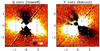 |
Fig. 32. Binned R Aqr I-band Stokes Q (left) and U (right) map extending over the whole detector of 3.6″×3.6″ detector area. The dashed boxes are the 1.8″×1.8″ areas shown in the large panels of Fig. 31. |
SPHERE/ZIMPOL allows for polarimetric observations with field angle offsets or polarization angle offset, which are both powerful methods to disentangle instrumental effects from weak but real sky signals.
5.6.3. Quantitative analysis for a radial cut
This section gives a quantitative analysis for the R Aqr polarization signal along the dashed line plotted in the large Qcoro-image (Fig. 31) through the strong dust feature in the North. In the corresponding Ucoro-frame, we inserted along the same direction artificial point signals, marked with horizontal dashes, for the evaluation of the detection limits of faint, polarized point sources.
Measured surface brightness and sensitivity limit. Figure 33 shows the radial cuts I(r, 7 ° ) and Q(r, 7 ° ) for the “nb”-, “sat”- and “coro”-images. For this 1-dim. profile extraction the reduced images were rotated by 7°, so that the cuts are simple mean profiles of 5 vertical columns from the central source at r = 0 to the upper edge at r = 500 pix. This cut through the northern dust cloud at r ≈ 120 pix avoids the strong vertical frame transfer trail in the non-coronagraphic images. The cloud, is not visible in the intensity profile, but appears as very strong, high signal-to-noise polarization source in polarimetric differential imaging. The profiles in Fig. 33 are given in flux normalized counts ctn6 like in Figs. 8 and 13 and the dotted curve is the 1-σ photon noise limit σ(Qcoro) for the “coro”-profile.
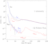 |
Fig. 33. Radial profiles for R Aqr for the ϕ = 7°-direction through the bright scattering clouds in the north as indicated in Fig. 31. |
Table 14 lists for selected areas along the profile the measured ctn6-values for I(r) and Q(r), the fractional polarization Q(r)/I(r), and the corresponding surface brightness contrast CPSF(r) for the intensity and CSB for the polarization in magnitudes. Note, that the sign of the Q-Stokes flux signal is negative in the North of the central source.
Normalized mean counts ctn6 for the PSF surface brightness of R Aqr and the polarized surface brightness of the circumstellar region along the position angle ϕ = 9° for the frames for the intensity Inb, Isat, and Icoro and the polarized flux Qnb, Qsat, and Qcoro.
The three intensity profiles Inb, Isat, and Icoro (Fig. 33 and Table 14) show quite some differences at small separations which reflect most likely the atmospheric and AO variations between the Inb and Isat frames, and the suppression of the PSF diffraction rings for Icoro. Despite this, the three Q-profiles agree very well at r = 30 pix and for Qsat and Qcoro also at 80 pix (Qnb(80 pix) is dominated by read-out noise). This confirms the finding from Fig. 31, that the “nb”-, “sat”-, and “coro”-frames are matching very well and provide a continuous mapping of the differential polarization signal from the center r = 0 to large separations r > 250 pix ( ρ > 0.9″).
Table 14 lists in italic letters the I(r)- and Q(r)-values with the highest signal-to-noise, which are not affected by saturation or attenuation by the coronagraph. The polarized surface brightness of the circumstellar dust is about 50–500 times lower than the intensity of the stellar PSF as follows from the fractional polarization Q(r)/I(r). This ratio depends on the PSF and therefore the variable AO performance and is not very useful for the characterization of the circumstellar scattering.
The polarized surface brightness contrast CSBpol is a better quantity to describe the polarized radiation from the dust (Sect. 5.1). For a region north of the central light source we can approximate CSBpol(r)≈ − Q(r)/Istar where Istar is the total stellar intensity as measured in an aperture of 3″-diameter. The obtained values range from SBpol − mstar = 4.0 to 12.4 mag arcsec−2 for the separation range from ρ = 0.11″ to 1.73″ (Table 14). This surface brightness in polarized flux is up to 19m fainter than the surface brightness of the PSF intensity peak CSB(0)= − 6.6m.
The R Aqr “coro”-images presented here are not really deep data, because they consist only of nDIT = 40 frames or ttotal = 400 s of integration for Q and the same for U. A comparison of R Aqr with other SPHERE/ZIMPOL polarimetric data in the literature shows that CSBpol is about 1 − 2 mag higher (relative emission Qcs/Istar, Ucs/Istar fainter) than the bright rims of bright proto-planetary disks, like HD 135344B with CSBpol ≈ 5 mag arcsec−2 at ρ = 0.2″ (Stolker et al. 2016), or HD 142527 with ≈7 mag arcsec−2 at ρ = 0.9″ (Avenhaus et al. 2017). Compared to these disk systems, the R Aqr central star is a bright source and therefore a comparable or better contrast is achieved with a short integration time. An about 2 mag higher contrast (fainter signals) of CSBpol ≈ 7.6 mag arcsec−2 at ρ = 0.3″ or 9.5 mag arcsec−2 at ρ = 1.2″ is measured for the debris disk HIP 79977 (Engler et al. 2017).
Detection limits for point sources. For the determination of the point source contrast limit, we use the U-image, which serves as low background observation for the ϕ = 7° profile direction. We insert in the U-frames artifical point sources at r = 30, 80, 120, 240, and 480 pixels and the U-polarization signals shown in Fig. 31 are ctn6 = 0.058 ct pix−1 corresponding to a polarization contrast of Cpol = fpol/fstar = 10−5 (Δm = 12.5m) for r = 80, 120 and 240 pix and ctn6 = 0.29 ct pix−1 at r = 30 (see Table 14).
The 5σ contrast limits Cpol(r)=U5σ(r)/Istar for polarized point sources are then derived by measuring the extracted signal similar to the measurements of α Hya B in Sect. 4.3 for artifical point sources with a range of U-fluxes. This yields the 5σ limits of Δm ≈ 12.6m, 13.0m or 14.9m at separations of 0.29″, 0.43″, or 0.86″, respectively (Table 14).
These are contrast limits comparable to the limits reported by van Holstein et al. (2010) for polarimetric observations of the HR 8799 planets in the near-IR with SPHERE/IRDIS. For separations ρ ≳ 0.6″ the ZIMPOL and IRDIS polarimetric modes are for bright targets essentially photon noise limited. Thus, deeper polarimetric contrast limits can be achieved, if more photons are collected with longer integrations or with observations of brighter targets. At small separations ρ ≲ 0.6″, there is in the R Aqr polarimetry data presented here, some residual speckle noise besides the photon noise, because our simple test data are not optimized for deep contrast limits. ZIMPOL was designed for the photon noise limited search of polarized light from extra-solar planets around very bright stars ≲3m based on a large number of well illuminated frames nDIT > 5000 and long total integration times ttotal > 3 h (Schmid et al. 2006a; Thalmann et al. 2008). Thus, the real polarized point source contrast limit of SPHERE/ZIMPOL can only be demonstrated with such long integration of very bright stars using coronagraphy and fast modulation polarimetry and more elaborate observing strategies than the simple “one HWP2-cycle” test used for our R Aqr.
A non-polarimetric ZIMPOL point source observation using angular differential imaging (ADI) of PZ Tel A and B is described in Maire et al. (2016). This system with a separation of ρ = 0.48″ has in the R_PRIM band a contrast of Δmag = 9.7m. The companion is detected with 30 min of integration in one ZIMPOL arm, with only 14° of field rotation and under mediocre > 1.1″ seeing conditions. Companions with much higher contrast of at least Δmag ≈ 12.5m should be observable with ZIMPOL ADI if data are taken under better conditions and a better observing strategy.
6. Discussion
This paper presents a detailed description of the SPHERE/ ZIMPOL instrument to support and promote scientific investigations based on new or archival observations. The provided information should also be helpful to optimize observing and data reduction strategies, for an evaluation of the performance of this instrument for possible upgrades (e.g. Lovis et al. 2017), or the design of more advanced systems for future telescopes like the ELT (Kasper et al. 2013; Keller et al. 2010).
High contrast and high resolution observations from the ground require the combination of an adaptive optics system with coronagraphy, and a differential imager for speckle noise suppression. All these methods are tricky, because the resulting performance depends on the target brightness, the atmosphere, the selection of the coronagraph, the mode of the differential imager, and on the appropriate observing strategy. It is not possible to describe such a complex system and its performance in a single paper, or a compact user manual. This paper provides a comprehensive hardware description, and highlight three important aspects, which are particularly special for the SPHERE/ZIMPOL instrument when compared to other AO-imaging systems: (i) the characterization of the PSF-properties in the visual provided by the SPHERE AO system and the VLT telescope, (ii) the performance of the visual coronagraph, and (iii) the polarimetric measuring strategy and data characteristics of the ZIMPOL system.
More technical information about ZIMPOL will become available in the future: a paper on the astrometric calibration is in preparation, and a description of photometric parameters is planned. Schmid et al. (2017) describe many technical aspects on the Hα imaging and absolute photometric measurements in several filters. Further, we expect that useful performance characteristics of SPHERE/ZIMPOL can be extracted from science papers, which aim for accurate measurements or push the performance of this instrument to the limits.
6.1. Key performance properties of ZIMPOL
SPHERE/VLT is one of the new generation extreme AO-systems available at large telescopes. The quality of the obtained PSFs depend strongly on the AO-system, the atmospheric conditions and the guide star magnitude mR and Table 7 characterizes the visible performance of the AO system for several typical cases using simple measuring parameters, e.g. the normalized PSF peak flux ctn6(0). Good corrections with ctn6(0)/106 > 0.3% (Strehl ratio ≳15% in the R-band) are achieved for stars down to mR ≈ 8m with an atmospheric seeing of ≈1″. For bright stars mR < 7m and good seeing conditions < 0.8″ the relative peak flux is twice as good ctn6(0)/106 > 0.6% and this corresponds to Strehl ratios of ≈30 − 50% in the R-band (see also Fusco et al. 2016). This provides for SPHERE/ZIMPOL a point source contrast performance of Δm ≈ 12.5m outside 0.15″ for the polarized flux (Table 14). The existing ADI-data of the PZ Tel binary Maire et al. (2016a) indicate, that similar contrasts performance are also possible for the intensity signal of a point source. For extended polarized emission, the system reaches outside of 0.15″ surface brightness contrast limits better than CSBpol > 7.5m arcsec−2.
The most outstanding property of SPHERE/ZIMPOL is the spatial resolution of up to 20 mas surpassing all other imaging instruments available at the VLT (de Zeeuw 2016). This limit can even be improved with sparse aperture masking, which is one of the most recent upgrades of the SPHERE/ ZIMPOL system (Cheetham et al. 2016). Observations with even higher resolution requires currently interferometric observations.
Visual extreme AO-systems are also available at other observatories, e.g. the pioneering MagAO-system at the Magellan telescope (Close et al. 2013), or SCExAO at the Subaru telescope (Jovanovic et al. 2015). Scientifically important features shared by all these visible AO systems is the access to the strong Hα emission line, and the extension of high resolution observations from the traditional near/mid-IR to the visible wavelength range (see Close 2016). There will be some healthy competition between these systems, but much more important is the mutual benefit in establishing common calibration targets, improving and checking measuring strategies and data reduction, and enhancing the science return thanks to complementary performance characteristics.
Many properties of the ZIMPOL system are quite typical for high resolution imagers using AO and they are not repeated here. We list here the special features of ZIMPOL:
-
a small detector pixel scale of 3.6 mas × 3.6 mas, giving 77160 pix arcsec−2 for each detector and a high full well photo-electron capacity of 7 × 10⁵ e− pix−1, allowing for efficient high contrast observations of the circumstellar regions of bright stars mR < 8m in broad band filters,
-
dual beam imaging and polarimetry for simultaneous observation with two cameras with many different options for the combination of filter bands, for example the combination of 1 nm or 5 nm Hα filters with a Hα continuum filter for spectral differential imaging. Alternatively, also narrow band filters can be combined with broad band filters for simultaneous, and therefore accurate flux measurements of the bright component in a high contrast system. For example, a bright star can be observed with the narrow Cnt820 or Cnt_Ha filters in one arm, and the faint companion or circumstellar features in the second arm with the corresponding broad band filter I_PRIM or R_PRIM, respectively,
-
a high resolution imaging polarimeter based on a fast modulation-demodulation technique for speckle noise suppression allowing high precision, Δp ≲ 10−4, broad-band polarimetry,
-
an innovative concept for the compensation and control of the instrument polarization effects providing absolutely calibrated linear polarization measurements with an accuracy of about ±0.1% for the relative Stokes parameters Q/I and U/I, despite the fact that SPHERE/ZIMPOL is a polarimetrically complex instrument at the Nasmyth focus.
-
the status of SPHERE/ZIMPOL as an ESO/VLT facility instrument, which ensures a well monitored and characterized system, steady improvements of the instrument operation, high standards for the execution of the observations and data calibration, a well established and user-friendly data archiving, and hopefully a long life-time. Another huge benefit is the large ESO user community using this system for a wide range of science targets with innovative observing strategies.
6.2. Possible instrument upgrades
Some evolution of the ZIMPOL system capabilities can be expected in the near future, because they can be realized without much effort. Very desirable would be the availability of the ZIMPOL off-axis fields shown in Fig. 3, which are currently not offered as user mode. This would provide the possibility to extend the field of view for more extended objects to a diameter of 8″, matching better the 11″×12.5″ field offered by the infrared channel SPHERE/IRDIS.
A very useful upgrade would be the availability of a low read-out noise mode for imaging, equivalent to the slow modulation polarimetric mode with low detector gain. Especially, low flux measurements taken in narrow band and line filters, as well as observations in the off-axis fields outside the light halo of the bright central star would profit because they are often read-out noise limited. Just taking long integrations > 5 min with a running AO system is critical because a few seconds of strongly reduced AO-performance or even an AO open loop, caused for example by a particularly bad atmospheric turbulence event, can degrade an entire long integration with an enhanced background of light from the central star. Another problem of long integrations are small pointing drifts of ≳10 mas which cause image smearing and this would be avoidable with shorter integrations and a realignment of individual frames in the data reduction.
Another type of quite easy instrument upgrades are new filters or coronagraphic masks in the exchange wheels of ZIMPOL or the visual coronagraph, respectively. New science cases may emerge, which call for filter changes, or better coronagraphic concepts could be implemented (e.g. Patapis et al. 2018).
Of course, most relevant would be any upgrades to the AO system or any other effort to improve the AO performance, like the suppression of the low wind effect with changes to the telescope (Sauvage et al. 2016a). Better wavefront corrections for SPHERE based on new software or hardware would be particularly beneficial for the short-wavelength ZIMPOL subsystem where typical Strehl ratios are ≲50% with quite some room for improvements.
6.3. New research opportunities offered by SPHERE/ZIMPOL
The special technical properties of SPHERE/ZIMPOL offer many new research opportunities, some are unique to this instrument and some are shared with the other visible light AO systems mentioned above. At least, the visual ZIMPOL observations are complementary to the data from the SPHERE near-IR focal plane instruments IRDIS and IFS, or other near-IR AO systems like for example Gemini/GPI (Macintosh et al. 2014) or Subaru SCExAO (Jovanovic et al. 2015), by extending the wavelength domain of high resolution and high contrast imaging towards shorter wavelengths. In the following, we provide an incomplete list of science topics where SPHERE/ZIMPOL is already providing or will provide interesting or even very important contributions in high contrast imaging. In this discussion on science opportunities one should not forget the technical requirement that SPHERE/ZIMPOL observations need a bright central star mR ≲ 9m for the AO wavefront sensing and that the system provides only a quite limited field of view ρ < 4″.
6.3.1. Search for extra-solar planets in reflected light
ZIMPOL was selected by the European Southern Observatory for the SPHERE VLT “planet finder” instrument with the mandate to explore the detection limits of high contrast polarimetric imaging for the search of reflected light from extrasolar planets (Schmid et al. 2006a). The aim of this unique instrument is to reach a contrast limit between the polarized flux of the planet ppl × Ipl and the total flux of a star Istar of
within an angular separation smaller than ρ < 1″. This limit would allow a detection of a Jupiter-sized giant planet or even terrestrial planets with a physical separation of 0.5 − 1 AU around one of the nearest bright stars (Thalmann et al. 2008; Milli et al. 2013). This aim defined many of the ZIMPOL design decisions and therefore this imager is tuned for the detection of very faint polarization sources near very bright stars.
The SPHERE-team carries out as part of their guaranteed time observations obtained for building the instrument, an investigation of the achievable detection limits of for the search of extra-solar planets. Very high contrast observations of a small number of targets are currently taken. The data confirm that ZIMPOL can reach at least for separations ρ > 0.5″ the above mentioned detection limit. The short test observations of R Aqr described in the previous section give already an impression of the high contrast performance in polarimetric imaging. SPHERE/ZIMPOL is pioneering this technique and the achievable contrast limits are certainly of interest for other high contrast search programs targeting the reflected light from extra-solar planets and for the planning of future instruments. Whether a successful detection will be possible with SPHERE/ZIMPOL depends on the presence of favorable planets within about 5 pc and further progress in the observations and data analysis.
6.3.2. Differential polarimetric imaging of circumstellar disk.
Disks around young stars are a primary science case for the SPHERE instrument and differential polarimetric imaging is a powerful technique for high contrast disk observations (e.g. Kuhn et al. 2001; Perrin et al. 2009; Quanz et al. 2011; Muto et al. 2012). The high spatial resolution and the high polarimetric sensitivity of ZIMPOL are ideal for the mapping of faint circumstellar disks in polarized light. The visual ZIMPOL data can be combined with near-IR observations, for example from SPHERE/IRDIS, to study the color dependence of the reflected light from protoplanetary disks around young stars like for example HD 135344B or TW Hya (Stolker et al. 2016; van Boekel et al. 2017).
Let us compare for this important science case the pro and cons for the ZIMPOL and IRDIS polarimetry modes for the differential polarimetric imaging of circumstellar disk, focussing on detecting a disk and mapping structural features. For fainter central stars mR > 8m IRDIS polarimetry provides as important advantage a significantly better AO performance, because all light in the 500–900 nm range can be used for the wave front sensing. The ZIMPOL science channel shares this light with the WFS and therefore only 21% of the flux is available for the WFS, if the gray beam splitter is used, or about 80% for the dichroic beam splitter. Another advantage of IRDIS is the larger field of view of 11″×11″, about ten times larger than the 3.6″×3.6″ detector field of view of ZIMPOL, or much more efficient than using multiple field observations inside the 8″ diameter instrument field of view. On the other side, the main advantages of ZIMPOL polarimetry when compared to IRDIS or other IR-polarimeters are the higher spatial resolution and the very good speckle noise suppression by the fast-modulation polarimetry techniques as described in this paper for R Aqr. Therefore, a higher contrast can be obtained for circumstellar disk around bright stars in the separation range ρ ≈ 0.02″−0.2″ and a good example is the detection of the inner disk of HD 142527 by Avenhaus et al. (2017). For disks around bright stars, ZIMPOL is at least competitive for the separation range ρ ≈ 0.2 − 2.0 as demonstrated for the faint debris disks HIP 79977 (Engler et al. 2017), but also for the innermost regions of bright protoplanetary disks, like HD 100457 (Benisty et al. 2017). In addition, ZIMPOL provides a more advanced polarimetric concept than IRDIS or other AO-assisted polarimetric imagers, allowing an easier calibration of polarimetric data and a quantitative analysis of the polarized reflectivity of the scattering dust.
6.3.3. Mass loss from red giants
The combination of high spatial resolution and sensitive polarimetry is ideal for the mapping of the light scattering from the circumstellar dust with SPHERE/ZIMPOL (e.g. Kervella et al. 2015; Khouri et al. 2016; Ohnaka et al. 2017a). As shown in Sect. 5.6 for R Aqr, the polarized light from dust scattering can be measured over a very wide separation range, and asymmetries, clumps and their evolution can be investigated in much detail. This important information from high resolution polarimetry, which was pioneered with interferometric observations by Ireland et al. (2005), or sparse aperture masking by Norris et al. (2012), is now also available with “simple” imaging. Such observations could be particularly useful for investigations and the modeling of the complex dust formation process in pulsating AGB stars (e.g. Aronson et al. 2017; Höfner et al. 2016; Höfner 2008).
Light scattering observations are highly complementary to observations of the thermal emission of the circumstellar dust in the mid-IR with e.g. the VLTI/MIDI interferometer (Paladini et al. 2017). AO observations in the visual achieves a comparable or even better resolution than mid-IR interferometry and is therefore well suited for the mapping of the complex distribution of circumstellar dust near the mass losing star. The visible range is ideal for the small dust particles formed around mass-losing red giants because they scatter much more efficiently short wavelength light. A technical challenge for very bright red giants are detector saturation issues. Red giants are much fainter in the visual and the ZIMPOL system is designed especially for high contrast observations of very bright targets and therefore also for the investigation of the brightest, most extended, nearby red giants.
6.3.4. Emission lines in stellar jets and outflows
Stellar jets and outflows produce often Hα and other emission lines from shocks or photoionized regions. ZIMPOL line filters are available for the Hα 656 nm, [O I] 630 nm, and HeI/NaI 588/589 nm lines which may serve as tracer of different types of ionized or partially ionized gas.
Achieving high contrast and high resolution observations in line filters is important for stellar jets from young stars (Frank et al. 2014) to access the innermost 10 AU where the outflow is not yet significantly perturbed by the interaction with the ambient medium. This requires line observations at separations below 70 mas for sources in nearby star-forming regions. Observing the innermost flow morphology is important to pinpoint the initial ejection site of the matter, e.g. a stellar wind, an “X-wind” from the inner edge of the disk, or a disk wind, which is then further accelerated and collimated by the combined action of magnetic fields and rotation (Ferreira et al. 2006). A first demonstration of the ZIMPOL potential on this topic is provided in Antoniucci et al. (2016) with Hα and [O I] observations of the young binary Z CMa. The authors could trace the collimated jet from one of the components down to ∼70 mas from the driving source, revealing a jet wiggling on time-scales of a few years, which may be induced by a non-detected close-in companion.
For many astronomical objects countless imaging data allready exists of the circumstellar line emission in the visual wavelength region taken with ground-based or space telescopes. The line observations of R Aqr provide a good example for the complementarity of emission line imaging with the SPHERE/ZIMPOL AO system (Schmid et al. 2017), with HST imaging (Melnikov et al. 2018), and with seeing limited imaging (Liimets et al. 2018).
6.3.5. Resolving the atmosphere of red giants.
The most extended red giant stars can be resolved with “simple ZIMPOL imaging” with a resolution of up to 20 mas as demonstrated for example for R Dor (Khouri et al. 2016) or α Ori (Kervella et al. 2016). “Simple imaging” because one can take many images in several filters within a few minutes, select the best data and measure wavelength dependencies. Geometric features, such as large spots or polar and equatorial zones, can be investigated and flux ratio maps can be obtained with simultaneous differential imaging, in e.g. the TiO_717 and Cnt748 band filters which sample cold and hot surfaces regions, or the N_Ha and CntHa filter pair for possible signs of shock heating. The “simple imaging” is also ideal for a monitoring program of the temporal evolution of surface features in these stars. Even better spatial resolution ρ < 20 mas should be achievable with sparse aperture masking or with advanced data analysis techniques. For these reasons the “simple”, ≈20 mas resolution, SPHERE/ZIMPOL imaging of extended red giant atmospheres provides useful complementary information with respect to the higher resolution, but much harder to obtain interferometric data (e.g. Haniff et al. 1995; van Belle et al. 1996; Ohnaka et al. 2017b).
6.3.6. Close binary stars.
For very close binary stars, the ≈20 mas spatial resolution of SPHERE/ZIMPOL is of course very useful for orbit determinations and the photometry of the individual components (e.g. Janson et al. 2018). A particular niche for the visual ZIMPOL instrument, when compared to near-IR AO instruments, are faint, hot companions to red stars, like white dwarfs companions to Ba-star, or Hα emitting active components to M-giants like the symbiotic system R Aqr shown in Fig. 6 (see also Schmid et al. 2017). The relative position between roughly equal flux (|log(f1/f2)| ≲ 1) hot and cold binary components can certainly be determined for separations of ≈10 mas or even smaller with simultaneous measurements of the combined binary PSF in a visual and a red filter. Photocenter differences between two bands might even be measurable at the milli-arcsec level, if other stars in the field or the features of a coronagraphic mask can be used as relative astrometric reference.
6.3.7. Solar system objects.
The SPHERE AO system is capable to lock on moving solar system objects if they are bright enough mR ≲ 10m and not too extended ≲2″. This was demonstrated during the SPHERE commissioning for Titan3 which has a diameter of ρ = 0.8″ and even Neptune with ρ = 2.4″ (Fusco et al. 2016). Thus, many bright asteroids, the Galilean moons, and Saturn’s moon Titan can be imaged in the visual. Sizes, shapes and surface structures can be investigated in much detail (Vernazza et al. 2008), and with enhanced resolution when compared to the near-IR range (e.g. Marchis et al. 2006), including the polarimetric properties of the reflecting terrains.
6.4. Conclusions
SPHERE/ZIMPOL is a very versatile adaptive optics instrument and we therefore expect many exciting new scientific results from this instrument. The above listed technical performances, upgrade options, and science topics give only a few examples of possible observational projects with this instrument.
Observational results based on adaptive optics profit a lot from the much enhanced spatial resolution and this provides since many years a continuous string of new detections (see Davies & Kasper 2012). The description of SPHERE/ZIMPOL given in this paper should help to define the best observing strategy for reaching deeper detection limits for new discoveries with AO observations at very high spatial resolution in the visual, using polarimetric imaging, angular or differential imaging with broad band, narrow band, or line filters.
On the other side, accurate quantitative measurements with AO systems are often difficult, because of the strongly variable atmospheric conditions and the resulting system performance. Particularly problematic is the photometry for very faint companions or extended circumstellar features for which simultaneous or quasi-simultaneous differential measurements are impossible. This makes the accurate characterization of high contrast objects in different wavelength bands, taken often with different instruments and usually under different atmospheric conditions very difficult and often uncertain. A lot of effort is required to describe AO observations accuratly and in a reproducible way but this is required for a detailed characterization of high contrast objects. This paper provides therefore a lot of technical information for the accurate characterization and calibration of SPHERE/ZIMPOL measurements.
From Bernhard Halle Nachfl.
ESO press release www.eso.org/public/news/eso1417
Acknowledgments
HMS thanks Wolfgang Löffler, Universiteit Leiden, for very helpful discussions and comments about the Goos-Hähnchen shift and related effects. SPHERE is an instrument designed and built by a consortium consisting of IPAG (Grenoble, France), MPIA (Heidelberg, Germany), LAM (Marseille, France), LESIA (Paris, France), Laboratoire Lagrange (Nice, France), INAF – Osservatorio di Padova (Italy), Observatoire de Gen‘eve (Switzerland), ETH Zurich (Switzerland), NOVA (Netherlands), ONERA (France) and ASTRON (Netherlands), in collaboration with ESO. SPHERE was funded by ESO, with additional contributions from CNRS (France), MPIA (Germany), INAF (Italy), FINES (Switzerland) and NOVA (Netherlands). SPHERE also received funding from the European Commission Sixth and Seventh Framework Programmes as part of the Optical Infrared Coordination Network for Astronomy (OPTICON) under grant number RII3-Ct-2004-001566 for FP6 (2004–2008), grant number 226604 for FP7 (2009–2012) and grant number 312430 for FP7 (2013–2016). HMS, SH and NE acknoledge financial support from SNSF through grant 200020_162630. Part of this work has been carried out within the framework of the National Centre for Competence in Research PlanetS supported by the Swiss National Science Foundation. H.A. and S.P.Q. acknowledge the financial support of the SNSF.
References
- Aiello, A., Merano, M., & Woerdman, J. P. 2009, Phys. Rev. A, 80, 061801 [NASA ADS] [CrossRef] [Google Scholar]
- Akiyama, E., Muto, T., Kusakabe, N., et al. 2015, ApJ, 802, L17 [NASA ADS] [CrossRef] [Google Scholar]
- Amara, A., & Quanz, S. P. 2012, MNRAS, 427, 948 [NASA ADS] [CrossRef] [Google Scholar]
- Antoniucci, S., Podio, L., Nisini, B., et al. 2016, A&A, 593, L13 [NASA ADS] [CrossRef] [EDP Sciences] [Google Scholar]
- Appenzeller, I. 1968, ApJ, 151, 907 [NASA ADS] [CrossRef] [Google Scholar]
- Aronson, E., Bladh, S., & Höfner, S. 2017, A&A, 603, A116 [NASA ADS] [CrossRef] [EDP Sciences] [Google Scholar]
- Artmann, K. 1948, Ann. Phys., 437, 87 [CrossRef] [Google Scholar]
- Aspin, C., Schwarz, H. E., McLean, I. S., & Boyle, R. P. 1985, A&A, 149, L21 [NASA ADS] [Google Scholar]
- Avenhaus, H., Quanz, S. P., Schmid, H. M., et al. 2014, ApJ, 781, 87 [NASA ADS] [CrossRef] [Google Scholar]
- Avenhaus, H., Quanz, S. P., Schmid, H. M., et al. 2017, AJ, 154, 33 [NASA ADS] [CrossRef] [Google Scholar]
- Bailey, J., & Hough, J. H. 1982, PASP, 94, 618 [NASA ADS] [CrossRef] [Google Scholar]
- Bastien, P., Drissen, L., Menard, F., et al. 1988, AJ, 95, 900 [NASA ADS] [CrossRef] [Google Scholar]
- Bastien, P., Vernet, E., Drissen, L., et al. 2007, in The Future of Photometric, Spectrophotometric and Polarimetric Standardization, ed. C.Sterken, ASP Conf. Ser., 364, 529 [NASA ADS] [Google Scholar]
- Bazzon, A., Gisler, D., Roelfsema, R., et al. 2012, in Ground-based and Airborne Instrumentation for Astronomy IV, Proc. SPIE, 8446, 93 [Google Scholar]
- Bellini, A., Anderson, J., van der Marel, R. P., et al. 2014, ApJ, 797, 115 [NASA ADS] [CrossRef] [Google Scholar]
- Benisty, M., Stolker, T., Pohl, A., et al. 2017, A&A, 597, A42 [NASA ADS] [CrossRef] [EDP Sciences] [Google Scholar]
- Beuzit, J.-L., Feldt, M., Dohlen, K., et al. 2008, in Ground-based and Airborne Instrumentation for Astronomy II, Proc. SPIE, 7014, 18 [Google Scholar]
- Bliokh, K. Y., & Aiello, A. 2013, J. Opt., 15, 014001 [NASA ADS] [CrossRef] [Google Scholar]
- Boccaletti, A., Abe, L., Baudrand, J., et al. 2008, in Adaptive Optics Systems, Proc. SPIE, 7015, 70151B [Google Scholar]
- Bonnefoy, M., Zurlo, A., Baudino, J. L., et al. 2016, A&A, 587, A58 [NASA ADS] [CrossRef] [EDP Sciences] [Google Scholar]
- Born, M., & Wolf, E. 1999, in Principles of Optics (Cambridge: Cambridge University Press) [Google Scholar]
- Brandner, W., & Hormuth, F. 2016, in Astronomy at High Angular Resolution, eds. H. M. J. Boffin, G.Hussain, J.-P. Berger, & L. Schmidtobreick Astrophysics and Space Science Library, 439, 1 [NASA ADS] [CrossRef] [Google Scholar]
- Breckinridge, J. B., Lam, W. S. T., & Chipman, R. A. 2015, PASP, 127, 445 [NASA ADS] [CrossRef] [Google Scholar]
- Cheetham, A. C., Girard, J., Lacour, S., et al. 2016, in Optical and Infrared Interferometry and Imaging V, Proc. SPIE, 9907, 99072T [CrossRef] [Google Scholar]
- Clarke, D., Stewart, B. G., Schwarz, H. E., & Brooks, A. 1983, A&A, 126, 260 [NASA ADS] [Google Scholar]
- Claudi, R. U., Turatto, M., Gratton, R. G., et al. 2008, in Ground-based and Airborne Instrumentation for Astronomy II, Proc. SPIE, 7014, 70143E [Google Scholar]
- Close, L. M. 2016, in Adaptive Optics Systems V, Proc. SPIE. 9909, 99091E [NASA ADS] [Google Scholar]
- Close, L. M., Males, J. R., Morzinski, K., et al. 2013, ApJ, 774, 94 [NASA ADS] [CrossRef] [Google Scholar]
- Collett, E. 1992, Polarized Light: Fundamentals and Applications (New York: Dekker) [Google Scholar]
- Cox, L. J. 1976, MNRAS, 176, 525 [NASA ADS] [Google Scholar]
- Davies, R., & Kasper, M. 2012, ARA&A, 50, 305 [NASA ADS] [CrossRef] [Google Scholar]
- de Juan Ovelar, M., Diamantopoulou, S., Roelfsema, R., et al. 2012, in Modeling, Systems Engineering, and Project Management for Astronomy V, Proc. SPIE, 8449, 844912 [CrossRef] [Google Scholar]
- de Zeeuw, T. 2016, The Messenger, 166, 2 [NASA ADS] [Google Scholar]
- Dixon, W. V. D., Davidsen, A. F., & Ferguson, H. C. 1995, ApJ, 454, L47 [NASA ADS] [CrossRef] [Google Scholar]
- Dohlen, K., Langlois, M., Saisse, M., et al. 2008, in Ground-based and Airborne Instrumentation for Astronomy II, Proc. SPIE, 7014, 70143L [CrossRef] [Google Scholar]
- Dohlen, K., Vigan, A., Mouillet, D., et al. 2016, Proc. SPIE, 9908, 99083D [Google Scholar]
- Engler, N., Schmid, H. M., Thalmann, C., et al. 2017, A&A, 607, A90 [NASA ADS] [CrossRef] [EDP Sciences] [Google Scholar]
- Ferreira, J., Dougados, C., & Cabrit, S. 2006, A&A, 453, 785 [NASA ADS] [CrossRef] [EDP Sciences] [Google Scholar]
- Frank, A., Ray, T. P., Cabrit, S., et al. 2014, Protostars Planets VI, 451 [Google Scholar]
- Fusco, T., Sauvage, J.-F., Petit, C., et al. 2014, in Adaptive Optics Systems IV, Proc. SPIE, 9148, 1 [Google Scholar]
- Fusco, T., Sauvage, J.-F., Mouillet, D., et al. 2016, in Adaptive Optics Systems V, Proc. SPIE, 9909, 99090U [CrossRef] [Google Scholar]
- Gandorfer, A. M. 1999, Opt. Eng., 38, 1402 [NASA ADS] [CrossRef] [Google Scholar]
- Gandorfer, A. M., & Povel, H. P. 1997, A&A, 328, 381 [NASA ADS] [Google Scholar]
- Garufi, A., Quanz, S. P., Schmid, H. M., et al. 2016, A&A, 588, A8 [NASA ADS] [CrossRef] [EDP Sciences] [Google Scholar]
- Gisler, D., Feller, A., & Gandorfer, A. M. 2003, in Polarimetry in Astronomy, Proc. SPIE, 4843, 45 [NASA ADS] [CrossRef] [Google Scholar]
- Gisler, D., Schmid, H. M., Thalmann, C., et al. 2004, in Ground-based Instrumentation for Astronomy, Proc. SPIE, 5492, 463 [Google Scholar]
- Goos, F., & Hänchen, H. 1947, Annal. Phys., 436, 333 [NASA ADS] [CrossRef] [Google Scholar]
- Haniff, C. A., Scholz, M., & Tuthill, P. G. 1995, MNRAS, 276, 640 [NASA ADS] [CrossRef] [Google Scholar]
- Höfner, S. 2008, A&A, 491, L1 [NASA ADS] [CrossRef] [EDP Sciences] [Google Scholar]
- Höfner, S., Bladh, S., Aringer, B., & Ahuja, R. 2016, A&A, 594, A108 [NASA ADS] [CrossRef] [EDP Sciences] [Google Scholar]
- Hsu, J.-C., & Breger, M. 1982, ApJ, 262, 732 [NASA ADS] [CrossRef] [Google Scholar]
- Ireland, M. J., Tuthill, P. G., Davis, J., & Tango, W. 2005, MNRAS, 361, 337 [NASA ADS] [CrossRef] [Google Scholar]
- Janson, M., Durkan, S., Bonnefoy, M., et al. 2018, A&A, submitted, [Google Scholar]
- Joos, F. 2007, PhD Thesis, ETH Zurich [Google Scholar]
- Joshi, U. C., Ganesh, S., & Baliyan, K. S. 2012, in Stellar Polarimetry: from Birth to Death, AIP Conference Proceedings, 1429, 222 [NASA ADS] [CrossRef] [Google Scholar]
- Jovanovic, N., Martinache, F., Guyon, O., et al. 2015, PASP, 127, 890 [NASA ADS] [CrossRef] [Google Scholar]
- Kasper, M., Beuzit, J.-L., Feldt, M., et al. 2012, The Messenger, 149, 17 [NASA ADS] [Google Scholar]
- Kasper, M., Kasper, M. & Mawet, D. 2013, in Proceedings of the Third AO4ELT Conference, 8 [Google Scholar]
- Keller, C. U., Schmid, H. M., Venema, L. B., et al. 2010, in Ground-based and Airborne Instrumentation for Astronomy III, Proc. SPIE, 7735, 77356G [CrossRef] [Google Scholar]
- Kemp, J. C., & Barbour, M. S. 1981, PASP, 93, 521 [NASA ADS] [CrossRef] [Google Scholar]
- Kervella, P., Domiciano de Souza, A., & Bendjoya, P. 2008, A&A, 484, L13 [NASA ADS] [CrossRef] [EDP Sciences] [Google Scholar]
- Kervella, P., Montargès, M., Lagadec, E., et al. 2015, A&A, 578, A77 [NASA ADS] [CrossRef] [EDP Sciences] [Google Scholar]
- Kervella, P., Lagadec, E., Montargès, M., et al. 2016, A&A, 585, A28 [NASA ADS] [CrossRef] [EDP Sciences] [Google Scholar]
- Khouri, T., Maercker, M., Waters, L. B. F. M., et al. 2016, A&A, 591, A70 [NASA ADS] [CrossRef] [EDP Sciences] [Google Scholar]
- Kuhn, J. R., Potter, D., & Parise, B. 2001, ApJ, 553, L189 [NASA ADS] [CrossRef] [Google Scholar]
- Lafrenière, D., Marois, C., Doyon, R., Nadeau, D., & Artigau, É. 2007, ApJ, 660, 770 [NASA ADS] [CrossRef] [Google Scholar]
- Langlois, M., Dohlen, K., Vigan, A., et al. 2014, in Ground-based and Airborne Instrumentation for Astronomy V, Proc. SPIE, 9147, 91471R [CrossRef] [Google Scholar]
- Law, N. M., Mackay, C. D., Dekany, R. G., et al. 2009, ApJ, 692, 924 [NASA ADS] [CrossRef] [Google Scholar]
- Liimets, T., Corradi, R. L. M., Jones, D., et al. 2018, A&A, 612, A118 [NASA ADS] [CrossRef] [EDP Sciences] [Google Scholar]
- Lovis, C., Snellen, I., Mouillet, D., et al. 2017, A&A, 599, A16 [NASA ADS] [CrossRef] [EDP Sciences] [Google Scholar]
- Macintosh, B., Graham, J. R., Ingraham, P., et al. 2014, Proc. Nat. Acad. Sci., 111, 12661 [Google Scholar]
- Maire, A.-L., Bonnefoy, M., Ginski, C., et al. 2016a, A&A, 587, A56 [NASA ADS] [CrossRef] [EDP Sciences] [Google Scholar]
- Maire, A.-L., Langlois, M., Dohlen, K., et al. 2016b, in Ground-based and Airborne Instrumentation for Astronomy VI, Proc. SPIE, 9908, 990834 [CrossRef] [Google Scholar]
- Malbet, F. 1996, A&AS, 115, 161 [NASA ADS] [Google Scholar]
- Marchis, F., Kaasalainen, M., Hom, E. F. Y., et al. 2006, Icarus, 185, 39 [NASA ADS] [CrossRef] [PubMed] [Google Scholar]
- Marois, C., Lafrenière, D., Doyon, R., Macintosh, B., & Nadeau, D. 2006, ApJ, 641, 556 [Google Scholar]
- Martinez Pillet, V., & Sanchez Almeida, J. 1991, A&A, 252, 861 [NASA ADS] [Google Scholar]
- McLaughlin, D. E., Anderson, J., Meylan, G., et al. 2006, ApJS, 166, 249 [NASA ADS] [CrossRef] [Google Scholar]
- Melnikov, S., Stute, M., & Eislöffel, J. 2018, A&A, 612, A77 [NASA ADS] [CrossRef] [EDP Sciences] [Google Scholar]
- Milli, J., Mouillet, D., Mawet, D., et al. 2013, A&A, 556, A64 [NASA ADS] [CrossRef] [EDP Sciences] [Google Scholar]
- Milli, J., Mouillet, D., Fusco, T., et al. 2017, Adapt. Opt. Extremely Large Tel., DOI 10.26698/AO4ELT5.0034 [Google Scholar]
- Momany, Y., Saviane, I., Smette, A., et al. 2012, A&A, 537, A2 [NASA ADS] [CrossRef] [EDP Sciences] [Google Scholar]
- Muto, T., Grady, C. A., Hashimoto, J., et al. 2012, ApJ, 748, L22 [NASA ADS] [CrossRef] [Google Scholar]
- Norris, B. R. M., Tuthill, P. G., Ireland, M. J., et al. 2012, Nature, 484, 220 [NASA ADS] [CrossRef] [PubMed] [Google Scholar]
- Ohnaka, K., Weigelt, G., & Hofmann, K.-H. 2017a, A&A, 597, A20 [NASA ADS] [CrossRef] [EDP Sciences] [Google Scholar]
- Ohnaka, K., Weigelt, G., & Hofmann, K.-H. 2017b, Nature, 548, 310 [NASA ADS] [CrossRef] [Google Scholar]
- Paladini, C., Klotz, D., Sacuto, S., et al. 2017, A&A, 600, A136 [NASA ADS] [CrossRef] [EDP Sciences] [Google Scholar]
- Patapis, P., Kühn, J., & Schmid, H. M. 2018, in Advances in Optical and Mechanical Technologies for Telescopes and Instrumentation III, Proc. SPIE, 10706, 107065J [Google Scholar]
- Perrin, M. D., Schneider, G., Duchene, G., et al. 2009, ApJ, 707, L132 [NASA ADS] [CrossRef] [Google Scholar]
- Perrin, M. D., Duchene, G., Millar-Blanchaer, M., et al. 2015, ApJ, 799, 182 [Google Scholar]
- Povel, H.-P. 1995, Opt. Eng., 34, 1870 [NASA ADS] [CrossRef] [Google Scholar]
- Povel, H., Aebersold, H., & Stenflo, J. O. 1990, Appl. Opt., 29, 1186 [NASA ADS] [CrossRef] [Google Scholar]
- Pragt, J., Roelfsema, R., Gisler, D., et al. 2012, in Ground-based and Airborne Instrumentation for Astronomy IV, Proc. SPIE, 8446, 844697 [NASA ADS] [CrossRef] [Google Scholar]
- Quanz, S. P., Schmid, H. M., Geissler, K., et al. 2011, ApJ, 738, 23 [NASA ADS] [CrossRef] [Google Scholar]
- Ragland, S., Le Coroller, H., Pluzhnik, E., et al. 2008, ApJ, 679, 746 [NASA ADS] [CrossRef] [Google Scholar]
- Rapson, V. A., Kastner, J. H., Millar-Blanchaer, M. A., & Dong, R. 2015, ApJ, 815, L26 [NASA ADS] [CrossRef] [Google Scholar]
- Riaud, P., Boccaletti, A., Baudrand, J., & Rouan, D. 2003, PASP, 115, 712 [NASA ADS] [CrossRef] [Google Scholar]
- Roelfsema, R., Schmid, H. M., Pragt, J., et al. 2010, in Ground-based and Airborne Instrumentation for Astronomy III, Proc. SPIE, 7735, 4 [Google Scholar]
- Roelfsema, R., Gisler, D., Pragt, J., et al. 2011, in Techniques and Instrumentation for Detection of Exoplanets V, Proc. SPIE, 8151, 81510N [Google Scholar]
- Roelfsema, R., Bazzon, A., Schmid, H. M., et al. 2014, in Ground-based and Airborne Instrumentation for Astronomy V, Proc. SPIE, 9147, 91473W [CrossRef] [Google Scholar]
- Roelfsema, R., Bazzon, A., Schmid, H. M., et al. 2016, in Adaptive Optics Systems V, Proc. SPIE, 9909, 990927 [NASA ADS] [CrossRef] [Google Scholar]
- Rouan, D., Riaud, P., Boccaletti, A., Clénet, Y., & Labeyrie, A. 2000, PASP, 112, 1479 [NASA ADS] [CrossRef] [Google Scholar]
- Sauvage, J.-F., Fusco, T., Rousset, G., & Petit, C. 2007, J. Opt. Soc. Am. A, 24, 2334 [NASA ADS] [CrossRef] [Google Scholar]
- Sauvage, J.-F., Fusco, T., Lamb, M., et al. 2016a, in Adaptive Optics Systems V, Proc. SPIE, 9909, 990916 [Google Scholar]
- Sauvage, J.-F., Fusco, T., Petit, C., et al. 2016b, J. Astron. Tel., Instrum. Syst., 2, 025003 [NASA ADS] [CrossRef] [Google Scholar]
- Scarrott, S. M., Warren-Smith, R. F., Pallister, W. S., Axon, D. J., & Bingham, R. G. 1983, MNRAS, 204, 1163 [NASA ADS] [CrossRef] [Google Scholar]
- Schiavon, R. P., Dalessandro, E., Sohn, S. T., et al. 2012, AJ, 143, 121 [NASA ADS] [CrossRef] [Google Scholar]
- Schmid, H. M., Beuzit, J.-L., Feldt, M., et al. 2006a, in Direct Imaging of Exoplanets: Science & Techniques, eds. C. Aime, & F. Vakili, IAU Colloq., 200, 165 [NASA ADS] [Google Scholar]
- Schmid, H. M., Joos, F., & Tschan, D. 2006b, A&A, 452, 657 [NASA ADS] [CrossRef] [EDP Sciences] [Google Scholar]
- Schmid, H.-M., Downing, M., Roelfsema, R., et al. 2012, in Ground-based and Airborne Instrumentation for Astronomy IV, Proc. SPIE, 8446, 8 [Google Scholar]
- Schmid, H. M., Bazzon, A., Milli, J., et al. 2017, A&A, 602, A53 [NASA ADS] [CrossRef] [EDP Sciences] [Google Scholar]
- Schneider, G., & Silverstone, M. D. 2003, in High-Contrast Imaging for Exo-Planet Detection, eds. A. B.Schultz, Proc. SPIE, 4860, 1 [NASA ADS] [CrossRef] [Google Scholar]
- Serkowski, K. 1974, in Planets, Stars, and Nebulae: Studied with Photopolarimetry, ed. T. Gehrels, IAU Colloq., 23, 135 [NASA ADS] [Google Scholar]
- Serkowski, K., & Shawl, S. J. 2001, AJ, 122, 2017 [NASA ADS] [CrossRef] [Google Scholar]
- Serkowski, K., Mathewson, D. S., & Ford, V. L. 1975, ApJ, 196, 261 [NASA ADS] [CrossRef] [Google Scholar]
- Sivaramakrishnan, A., Koresko, C. D., Makidon, R. B., Berkefeld, T., & Kuchner, M. J. 2001, ApJ, 552, 397 [NASA ADS] [CrossRef] [Google Scholar]
- Soummer, R., Pueyo, L., & Larkin, J. 2012, ApJ, 755, L28 [NASA ADS] [CrossRef] [Google Scholar]
- Stenflo, J. O. 1996, Nature, 382, 588 [NASA ADS] [CrossRef] [Google Scholar]
- Stenflo, J. O., & Keller, C. U. 1997, A&A, 321, 927 [NASA ADS] [Google Scholar]
- Stolker, T., Dominik, C., Avenhaus, H., et al. 2016, A&A, 595, A113 [NASA ADS] [CrossRef] [EDP Sciences] [Google Scholar]
- Thalmann, C., Schmid, H. M., Boccaletti, A., et al. 2008, in Ground-based and Airborne Instrumentation for Astronomy II, Proc. SPIE, 7014, 3 [Google Scholar]
- Thalmann, C., Mulders, G. D., Janson, M., et al. 2015, ApJ, 808, L41 [NASA ADS] [CrossRef] [Google Scholar]
- Tinbergen, J. 1979, A&AS, 35, 325 [NASA ADS] [Google Scholar]
- Tinbergen, J. 2007, PASP, 119, 1371 [NASA ADS] [CrossRef] [Google Scholar]
- van Belle, G. T., Dyck, H. M., Benson, J. A., & Lacasse, M. G. 1996, AJ, 112, 2147 [NASA ADS] [CrossRef] [Google Scholar]
- van Boekel, R., Henning, T., Menu, J., et al. 2017, ApJ, 837, 132 [NASA ADS] [CrossRef] [Google Scholar]
- van Holstein, R. G., Snik, F., Girard, J. H., et al. 2010, in Techniques and Instrumentation for Detection of Exoplanets VIII, Proc. SPIE, 10400, 1040015 [Google Scholar]
- Vernazza, P., Marchis, F., Carry, B., Marsset, M., & Hanus, J. 2008, in European Planetary Science Congress (EPSC2017), 11 [Google Scholar]
- Vigan, A., Langlois, M., Dohlen, K., et al. 2014, in Ground-based and Airborne Instrumentation for Astronomy V, Proc. SPIE, 9147, 91474T [CrossRef] [Google Scholar]
- Vigan, A., Bonnefoy, M., Ginski, C., et al. 2016, A&A, 587, A55 [NASA ADS] [CrossRef] [EDP Sciences] [Google Scholar]
- Whittet, D. C. B., Martin, P. G., Hough, J. H., et al. 1992, ApJ, 386, 562 [NASA ADS] [CrossRef] [Google Scholar]
- Wildi, F., Mouillet, D., Beuzit, J.-L., et al. 2009, in Techniques and Instrumentation for Detection of Exoplanets IV, Proc. SPIE, 7440, 74400Q [NASA ADS] [CrossRef] [Google Scholar]
- Wildi, F. P., Michaud, B., Crausaz, M., et al. 2010, in Ground-based and Airborne Instrumentation for Astronomy III, Proc. SPIE, 7735, 77352V [NASA ADS] [CrossRef] [Google Scholar]
- Zurlo, A., Vigan, A., Galicher, R., et al. 2016, A&A, 587, A57 [NASA ADS] [CrossRef] [EDP Sciences] [Google Scholar]
All Tables
Calibration measurements taken during the year 2015 for the modulation – demodulation efficiencies ϵftϵmod and ϵmod in various filters.
Pass-band filters, neutral density filters, and calibration components available in the filter wheels FW0, FW1 and FW2 of ZIMPOL.
Geometric parameters for the telescope pupil, the intermediate pupil, and the pupil stop masks in the SPHERE visual coronagraph.
Measurements of the flux ratio fB/fA and the (S/N)B of α Hyi A and B, using different coronagraphic configurations of SPHERE/ZIMPOL.
Measured and corrected polarization pc [%] and θc [°] of high-polarization standard stars and comparisons with literature values pℓ, θℓ.
Normalized mean counts ctn6 for the PSF surface brightness of R Aqr and the polarized surface brightness of the circumstellar region along the position angle ϕ = 9° for the frames for the intensity Inb, Isat, and Icoro and the polarized flux Qnb, Qsat, and Qcoro.
All Figures
|
Fig. 1. Block diagram of the SPHERE common path (CPI) up to the beam splitter vi.BS and the SPHERE visual channel. The blue color indicates exchangeable components, green are rotating components, and red components are only inserted for polarimetry. The ZIMPOL box is shown in detail in Fig. 2. |
| In the text | |
|
Fig. 2. Block diagram for ZIMPOL with exchangeable components plotted in blue, while red components are only inserted for polarimetry. |
| In the text | |
|
Fig. 3. Full ZIMPOL instrument field for the astrometric field 47 Tuc. The central detector field is plotted in black, while colors are used for the 8 pre-defined off-axis fields OAF1-OAF8. The off-axis fields have been shifted slightly (red to the left, blue to the right, and green up) for better visibility. No data are available for OAF4 because of an observational error. |
| In the text | |
|
Fig. 4. ZIMPOL principle: The modulator switches in one cycle n the polarization direction between I⊥ and I∥. The polarization beam splitter selects for each channel only one polarization mode so that a polarization signal is converted into an intensity modulation. The masked CCDs demodulate the signal with charge-shifting, which is synchronized with the modulator. |
| In the text | |
|
Fig. 5. Schematic setup of a small section of the ZIMPOL detector assembly with the stripe mask (red), the cylindrical micro lens array with the dashed focus line (blue) and the detector pixels (black). |
| In the text | |
|
Fig. 6. Raw counts for the central 40 × 40 pixel regions of the Hα images for the central R Aqr binary, separation 45 mas, taken in imaging mode (left) and in polarimetric mode (right). The dotted circles in the polarimetric data indicate spurious charge shifting effects. |
| In the text | |
|
Fig. 7. Transmission curves for the ZIMPOL color filters, the blocking filter and the dichroic beamsplitter. Black curves are used for filters located in FW1 and FW2, red for filters in FW0, blue are filters in FW1 only, and green filters in FW2 only. |
| In the text | |
|
Fig. 8. Normalized PSFs of HD 183143 for the V-band (top) and the N_I-band (bottom) with the color scale reduced by a factor of 100 for the central peak within r < 20 pixels. Marked PSF features are the speckle ring near the AO control radius (r), strong fixed speckles from the AO system (s), two telescope M2 spider features (t), and the CCD frame transfer trail of the PSF peak (c). The dashed rings illustrate the location of the azimuthal cuts shown in Fig. 9. |
| In the text | |
|
Fig. 9. Azimuthally averaged radial profiles ctn6( ρ) (left) and azimuthal profiles ctn6(r, ϕ) for r = 50, 80, 120 and 180 pix (right) corresponding to ρ = 0.18″, 0.29″, 0.43″, and 0.65″, respectively for the PSFs of HD 183143 shown in Fig. 8. Also indicated as gray shading are the standard deviations of the azimuthal points σ(ctn6(r, ϕ). The location of the azimuthal cuts are indicated in the ct6n(r)-panels and in Fig. 8. |
| In the text | |
|
Fig. 10. Flux normalized PSFs ctn6(r) for HD 183143 (thick profiles) and the calculated diffraction limited PSF of the VLT (thin profile) for the filters V (λ = 545 nm), N_R (645 nm), N_I (817 nm), and including the H-band (1.62 μm) for the VLT. One pixel is 3.6 mas. |
| In the text | |
|
Fig. 11. Same PSFs for HD 183143 and the VLT diffraction limit as in Fig. 10 but normalized to the peak flux. The dashed line in the left panel marks the half width at half maximum of the profiles. The dotted curves are the calculated diffraction limited profiles. The flux scale in the right panel is 100 times lower. |
| In the text | |
|
Fig. 12. Profiles for the normalized encircled flux Ef(r) for the same PSFs of HD 183143 and the VLT diffraction as in Fig. 10. The dashed lines illustrate the parameter Ef10. |
| In the text | |
|
Fig. 13. Normalized radial profiles ct6n for V- and N_I-band observations of HD 161096 with “excellent”, for HD 183143 with “good”, and HD 129502 with “bad” quality PSFs. |
| In the text | |
|
Fig. 14. Normalized PSFs for special cases: Panel a: VBB-filter image of HD 142527 as example for the low wind effect, panel b: faint star 47 Tuc MMS12 in I_PRIM, and panel c: a 10 ms snap-shot image of α Eri A and B in the line filter CntHa. The color scale is reduced by a factor of 100 for the PSF center within ρ < 0.072″. Axes are in arcsec. |
| In the text | |
|
Fig. 15. Images of the central part (1.8″×1.8″) of focal plane masks available in the visual coronagraph of SPHERE. The masks in the top row are deposited on a plate and the gray scale is enhanced to show the frequency of dust features on the masks. |
| In the text | |
|
Fig. 16. Coronagraphic images of α Hyi (1.8″×1.8″) for the I_PRIM-filter taken with the panel a: small S, panel b: medium M, panel c; large L, and panel d: extra-large XL focal plane masks of SPHERE All images are normalized ctn6 relative to the non-coronagraphic PSF and displayed with the same color scale. |
| In the text | |
|
Fig. 17. Normalized radial profiles ct6n(r) for the I_PRIM coronagraphic images in Fig. 16 of α Hyi taken with the small S (blue), medium M (green), large L (red), and extra-large XL (magenta) focal plane stops. Also plotted is the non-coronagraphic PSF profile. The dotted lines indicate the nominal mask radii. |
| In the text | |
|
Fig. 18. Pupil stop images for the SPHERE visual coronagraph taken with the internal point source and the pupil imaging lens. |
| In the text | |
|
Fig. 19. Images of the pupil plane (left) and the center of the focal plane (right) for a coronagraphic observation of α Hyi with the focal plane mask CLC-S-WF without pupil stop (top row) and with pupil stop (middle row). The bottom panels are the differences of the two upper panels. |
| In the text | |
|
Fig. 20. Vertical pupil intensity profiles Φ (top) and mean radial profiles f(r) (bottom) for the coronagraphic observation (CLC_S_WF) of α Hyi without pupil stop (black) and with stopB1_2 (blue). The red curve in the bottom panel shows the diffracted light in the focal plane which are suppressed by the pupil stop. |
| In the text | |
|
Fig. 21. α Hyi A and B observed in the I_PRIM filter with panel a: small and panel b; medium MT classical Lyot coronagraph, panel d: without coronagraph, while (panel c) was taken in the N_I band filter. and the four quadrant phase mask 4QPM2. The circles are flux apertures for component A (center), component B at ρ = 91 mas (black), while (panel a) shows also the concentric comparison apertures. North is up and east to the left. |
| In the text | |
|
Fig. 22. Coronagraphic images of α Hya taken in the R_PRIM filter, the CLC-S-WF coronagraph and with image rotation 0°, 60°, and 120° (upper row). The lower row shows the mean of the derotated images (left), the median of non-derotated image (middle), and the mean of the rotated difference between non-derotated image and non-derotated median (right) as result of a simple roll-angle angular differential imaging procedure. |
| In the text | |
|
Fig. 23. Residual telescope polarization qtel = Qtel/I and utel = Utel/I as function of parallactic angle for the unpolarized star ϵ Eri in the VBB filter. Also shown are the measurements q +, q −, u +, and u − of a polarimetric cycle, which include instrument polarization component ±pSZ for the P2-mode and a field position angle offset of 60°. |
| In the text | |
|
Fig. 24. Telescope polarization angle θtel as function of the parallactic angle for zero-polarization standard stars measured in the filters V (green), N_R (red), and N_I (black) with dotted lines for the best fits according to Eq. (20). Blue diamonds are the VBB-filter data from Fig. 23. |
| In the text | |
|
Fig. 25. Polarization of high polarization standard stars for the N_R filter: black symbols give efficiency or c1 corrected values while red symbols are also corrected for the telescope polarization (c2-correction). For individual targets, either plus-signs or diamonds are used in order to avoid confusion. Corresponding literature values are plotted as blue squares with error bars. Also included are the zero-polarization standard stars from the previous subsection. |
| In the text | |
|
Fig. 26. Observed polarimetric beamshift for a stellar PSF of α Cen B taken in June 2016 with the VBB and ND4 filters: The first row shows two consecutive polarization frames (Io − Ie)0 and (Io − Ie)Π taken with opposite, zero and pi demodulation phase shifts and the resulting, charge-trap corrected, Q+-frame. The third row illustrates the beamshift for the derotated Q+-, Q−-, and the final “science” Q-image. The second and bottom rows show the same but with the beamshifts corrected between the odd-row Io and even-row Ie sub-frames. |
| In the text | |
|
Fig. 27. Schematic and simplified illustration of the polarimetric beam shift effects for the M3 Nasmyth mirror. The incoming beam and the expected reflection according to geometric optics are plotted in black. The beam and wavefront displacements for I⊥ and I∥ caused by the phase shifts, with the corresponding “effective” mirror surface location and tilts, are hugely exaggerated and drawn in red and blue respectively. |
| In the text | |
|
Fig. 28. Beam shift effect for α Cen B in the VBB filter for a coronagraphic (CLC-MT-WF) Stokes Q frame (left) and the beam shift corrected frame (right) for essentially the same instrument configuration as the stellar PSF in Fig. 26. The arrow in the left panel points to the PSF peak transmitted through the mask. PSF residual features are marked in the left panel with “t” and “s” according to Fig. 8. In the right panel the arrow points to one of several spots from the camera, which show up because of the applied beam-shift correction. The squares at the bottom mark the area for the reported σ(Q). |
| In the text | |
|
Fig. 29. Stokes Q and U images for the V-band filter of the PSF standard HD 183143. These are the polarization images corresponding to the intensity PSF shown in Fig. 8. |
| In the text | |
|
Fig. 30. HD 183143 mean radial V-band profiles (left) for the Stokes flux Q(r) and U(r) (top) and the fractional polarization Q(r)/I(r) and U(r)/I(r) (bottom) and the corresponding azimuthal profiles Q(80, ϕ), U(80, ϕ), and Q(80, ϕ)/I(80, ϕ), U(80, ϕ)/I(80, ϕ) (left). The U-data are shifted downwards in for better visibility and the dashed lines indicate the offset. |
| In the text | |
|
Fig. 31. R Aqr I-band Stokes Q (left) and U (right) signal measured for the unsaturated PSF in the narrow-band (nb) Cnt820 filter (upper left), for the saturated broad band I_PRIM filter (middle left), and deep coronagraphic observations for the I_PRIM filter and slow polarimetry mode (lower left and large frame). The cut for the count profiles of Fig. 33 is shown in the large Q-frame. Units are in pixels of 3.6 mas. |
| In the text | |
|
Fig. 32. Binned R Aqr I-band Stokes Q (left) and U (right) map extending over the whole detector of 3.6″×3.6″ detector area. The dashed boxes are the 1.8″×1.8″ areas shown in the large panels of Fig. 31. |
| In the text | |
|
Fig. 33. Radial profiles for R Aqr for the ϕ = 7°-direction through the bright scattering clouds in the north as indicated in Fig. 31. |
| In the text | |
Current usage metrics show cumulative count of Article Views (full-text article views including HTML views, PDF and ePub downloads, according to the available data) and Abstracts Views on Vision4Press platform.
Data correspond to usage on the plateform after 2015. The current usage metrics is available 48-96 hours after online publication and is updated daily on week days.
Initial download of the metrics may take a while.