| Issue |
A&A
Volume 619, November 2018
|
|
|---|---|---|
| Article Number | A96 | |
| Number of page(s) | 8 | |
| Section | Planets and planetary systems | |
| DOI | https://doi.org/10.1051/0004-6361/201833567 | |
| Published online | 12 November 2018 | |
HD 189733 b: bow shock or no shock?★
Hamburger Sternwarte, Universität Hamburg, Gojenbergweg 112,
21029
Hamburg,
Germany
e-mail: This email address is being protected from spambots. You need JavaScript enabled to view it.
Received:
4
June
2018
Accepted:
23
August
2018
Abstract
Context. Hot Jupiters are surrounded by extended atmospheres of neutral hydrogen. Observations have provided evidence for in-transit hydrogen Hα absorption as well as variable pre-transit absorption signals. These have been interpreted in terms of a bow shock or an accretion stream that transits the host star before the planet.
Aims. We test the hypothesis of planetary-related Hα absorption by studying the time variability of the Hα and stellar activity-sensitive calcium lines in high-resolution TIGRE (Telescopio Internacional de Guanajuato Robótico Espectroscópico) spectra of the planet host HD 189733.
Methods. In the framework of an observing campaign spanning several months, the host star was observed several times per week randomly sampling the orbital phases of the planet. We determine the equivalent width in the Hα and Ca IRT(calcium infrared triplet) lines, and subtract stellar rotationally induced activity from the Hα time series via its correlation with the IRT evolution. The residuals are explored for significant differences between the pre-, in-, and out-of-transit phases.
Results. We find strong stellar rotational variation with a lifetime of about 20–30 days in all activity indicators, but the corrected Hα time series exhibits no significant periodic variation. We exclude the presence of more than 6.2 mÅ pre-transit absorption and 5.6 mÅ in-transit absorption in the corrected Hα data at a 99% confidence level.
Conclusions. Previously observed Hα absorption signals exceed our upper limits, but they could be related to excited atmospheric states. The Hα variability in the HD 189733 system is dominated by stellar activity, and observed signals around the planetary transit may well be caused by short-term stellar variability.
Key words: planets and satellites: atmospheres / planets and satellites: gaseous planets / planets and satellites: individual: HD 189733
Full Table 2 is only available in electronic form at the CDS via anonymous ftp to cdsarc.u-strasbg.fr (130.79.128.5) or via http://cdsarc.u-strasbg.fr/viz-bin/qcat?J/A+A/619/A96
© ESO 2018
1 Introduction
Today our knowledge about extrasolar planets is not only limited to basic parameters like mass and radius, but information on the chemical composition has also been derived from transmission spectroscopy in multiple cases (e.g., Sing et al. 2016). During transit, a planetary atmosphere causes excess absorption in atomic or molecular lines. In the extended atmospheres of large close-in gas planets, hydrogen remains mostly neutral and in the ground state, despite equilibrium temperatures of several thousand Kelvin, resulting in strong hydrogen line absorption. In fact, observations verified Lyα excess absorption around the transits of HD 189733 b (Lecavelier Des Etangs et al. 2010; Bourrier et al. 2013), HD 209458 b (Vidal-Madjar et al. 2003; Ehrenreich et al. 2008), and GJ 436 b (Kulow et al. 2014; Ehrenreich et al. 2015). For the aforementioned planets, transit depths of more than 10% were measured in the Lyα line wings, in contrast to broadband optical transit depth measurements of 0.6% for GJ 436 b and 2.5% for HD 189733 b (Han et al. 2014). Clearly, these planets must host extended envelopes of hydrogen.
These close-in planets are exposed to extreme high-energy irradiation levels, which are thought to drive a significant loss of atmospheric material through an energy-limited planetary wind (Watson et al. 1981; Lammer et al. 2003; Salz et al. 2016). Such a wind can carry considerable amounts of neutral hydrogen into elevated atmospheric layers. For example, interactions with the stellar wind could increase the local excitation level, which would lead to enhanced absorption in the Balmer lines. In contrast to the Lyα line, the Balmer series can be studied with ground-based telescopes equipped with medium-resolution spectrographs covering the visible wavelength range. Particularly, excess hydrogen Hα absorption has been claimed to occur around the transit of HD 189733 b (Jensen et al. 2012; Cauley et al. 2015).
Here we investigate possible Hα absorption in the HD 189733 system with a very general observing approach. In Sect. 2, we present the properties of HD 189733 and introduce the concept of a bow shock. In Sect. 3 we describe our dataset and go through the data reduction steps. We present our results and conclusions in Sects. 4 and 5.
2 The case of HD 189733 b
The K dwarf HD 189733 is orbited by a Jupiter-sized planet in 2.2 days, a so-called hot Jupiter. The host star is considerably more active than the Sun, although with a presumed age of 5.3 ± 3.8 Gyr it is not a young star(Bonfanti et al. 2016); we list the stellar and planetary properties in Table 1. The high level of stellar irradiation in the close planetary orbit leads to a bloated planetary atmosphere, which has been subject to intensive studies because of the stellar brightness (mV = 7.65). For example, Boisse et al. (2009) present a spectroscopic observing campaign, which was carried out with the high-resolution spectrograph SOPHIE (Spectrographe pour l’Observation des Phénomènes des Intérieurs stellaires et des Exoplanètes) mounted on the 1.93-m telescope at the Observatoire de Haute-Provence, to study the impact of stellar activity on RV (radial velocity) measurements. The authors concluded that the activity indices Ca H&K, He I, and Hα show a periodicity close to the stellar-rotation period of 12 days (Henry & Winn 2008). Boisse et al. also searched for planetary signals with a period of 2.2 days in these lines. The Hα variability was not found to change with the planetary orbital phase on a level of 2% over a 0.678 Å passband.
Later observations studied single transits in detail. Jensen et al. (2012) show a statistically significant Hα excess absorption signal during the transit of the hot Jupiter. Recently, Cauley et al. (2015) studied the planetary transit also covering several hours before and after the transit, and found Hα excess absorption during the pre-transit phase as deep as 10 mÅ and lasting about 2 h. In contrast, no absorption was found in the cores of the chromospheric activity indicators Ca H&K. Therefore, they concluded that the observed feature is related to an extended planetary atmosphere and not to stellar activity, and speculate that the transit of a bow shock could precede the transit of the planetary disk.
The presence of pre-transit absorption seems to be confirmed by additional data (Cauley et al. 2016), where an excess absorption depth of 7 mÅ over a duration of 2.5 h was detected in the pre-transit phase. Cauley et al. interpret this signal as accretion clumps spiraling toward the star, but also point out that this interpretation has serious limitations. Further investigations by Barnes et al. (2016) challenge the results and note that the Hα variations are well correlated with the Ca H&K lines, indicating that the Hα time series are dominated by stellar activity. Yet, additional out-of-transit time series taken by Cauley et al. (2017) show significantly lower Hα residual equivalent width than the previously presented pre-transit signals. Thus, in summary, the origin of the Hα features has to be treated as an open issue.
3 Observations and data reduction
3.1 Observations
To test the nature of the Balmer line absorption features in HD 189733, we initiated an observing campaign to monitor chromospheric and possibly planet-induced variations. The campaign was performed with our 1.2 m TIGRE (Telescopio Internacional de Guanajuato Robótico Espectroscópico) telescope located in the central Mexican highlands. TIGRE is equipped with a spectrograph with a nominal resolution of 20 000. For details about the spectrograph and telescope, we refer to Schmitt et al. (2014). The brightness of the host star allows us to reach a signal-to-noise ratio (S/N) of about 84 inside the Hα line core with typically 900 s exposures. The actual exposure times were varied according to the observing conditions to reach the required S/N.
We typically obtained several spectra of HD 189733 per week, randomly sampling the stellar rotation phase and the planetary orbit. Because the pre- and in-transit phases cover only a small fraction of the planetary orbit, we randomly increase the sampling rate around the transit phase. Therefore, during transit nights our goal was to take three spectra; if no transit was expected, we took a single exposure per night. The target is only observable from spring to fall and the weather is generally more unstable during the summer, causing larger observation gaps (see Fig. 1). Nevertheless, this is one of the most extensive spectral time series of HD 189733 to our knowledge. In total we acquired 108 spectra; the precise observing dates are listed in Table 2.
The raw CCD (charge-coupled device) frames are automatically reduced by the TIGRE reduction pipeline (Mittag et al. 2010), currently in version 3.1; it is based on the REDUCE package described in detail by Piskunov & Valenti (2002).
Parameters of HD 189733 and its planet b.
Observed excess equivalent width in different lines.
3.2 Telluric correction
In the visible and near infrared wavelength range, molecules like O2 and H2O cause telluric absorption that depends on the airmass and meteorological parameters such as relative humidity. To achieve the data qualityrequired for the study of planetary absorption, our first step is the correction of the telluric absorption lines, for which we use the ESO (European Southern Observatory) code molecfit (Smette et al. 2015). It works as follows: first, we choose wavelength regions that are heavily affected by telluric lines and show the least stellar lines. The wavelength ranges we use and the dominant telluric absorbers are given in Table 3. Strong stellar lines in these regions are masked. Molecfitcalculates a synthetic telluric absorption spectrum based on the HITRAN (high-resolution transmission) molecular database (Rothman et al. 2009). The code takes into account the spectrograph’s resolution, and local airmass, temperature, pressure, and humidity profiles from model atmospheres (Noll et al. 2013). The initially derived atmospheric transmission spectrum is the starting point of a χ2 minimization that typically converges after only a dozen iterations. The stellar spectrum is divided by the telluric transmission spectrum, which strongly reduces the equivalent width of telluric lines.
In the calcium infrared triplet lines located at 8498, 8542, and 8662 Å, the differences between corrected and uncorrected data are small, but this is not true for the Hα line. Earth’s barycentric motion in the direction of HD 189733 changes from −22.3 km s−1 in April to +8.4 km s−1 in August, which causes H2O absorption lines with equivalent widths of 3.5 and 4.5 mÅ to drift across the stellar Hα line. This is on the order of the observed changes in the equivalent width of the Hα line, therefore a proper correction is vital for our analysis. We note that the depth of an unsaturated telluric line can be modeled with an accuracy of better than 2% (Smette et al. 2015). This corresponds to an error of about 0.1 mÅ in the Hα equivalent width, which is small compared to the typical error margin. Therefore, telluric residuals introduce only a negligible error on the line equivalent width that is studied in the following.
Wavelength ranges for telluric column density fitting.
3.3 Derivation of the excess emission
Stellar chromospheric variations and planetary absorption manifest themselves as (subtle) changes in the equivalent width of sensitive lines. Calcium and hydrogen lines are among the most common stellar activity indicators. To subtract photospheric contributions, we compute the excess equivalent width within the cores of activity sensitive lines after the subtraction of an inactive template spectrum. Our template star is HD 10476 (see Fig. 2 for a comparison). In general, HD 10476 and HD 189733 are very similar, but HD 10476 is 2.4 mag brighter. A detailed listing of its properties can be found in Table 4. While metallicity and surface gravity are identical within the error bars, this is not true for the effective temperature(cf. Tables 1 and 4). As pointed out by Martin et al. (2017), the effective temperature difference has a negligible effect on our results. Our template star is an inactive, slow rotator with a  = −5.092. While small emission cores are visible in the Ca H&K lines, the core emission is much stronger in HD 189733. This leads to a systematic but constant underestimation of the absolute excess flux. Since we are only interested in the temporal evolution of the Hα excess, we could in principle also take an average spectrum of HD 189733 or a stellar model atmosphere as template. This would only cause a vertical offset of the data points in Fig. 1.
We follow the analysis of Martin et al. (2017) and summarize only the most important steps. After telluric correction, we normalize the spectra. In the case of the Hα line, we select the wavelength region from 6551 to 6580 Å. Inside this region we regard the upper envelope as continuum data points. To this envelope we fit a linear function that we use to normalize the whole region. Next, we perform a wavelength shift to bring object and template to a common wavelength grid by cross-correlating them. The template spectrum is artificially broadened to match the rotational broadening of HD 189733. Then we subtract the template from our HD 189733 observations. In most wavelength ranges, the residuals are zero within the error bars, but chromospheric excess emission of HD 189733 is present in the cores of activity sensitive lines. Next, we integrate the excess flux in the line cores using a 2 Å band in Hα and a 1.5 Å band in the other lines. The bands are chosen by visual inspection to cover the strongest excess flux in the line cores. The result is the excess equivalent width (see Table 2), which we use as activity indicator. The average S/N of the excess equivalent widths is about 18 in the Ca H&K, 36 in the Ca IRT, and 22 in the Hα region.
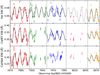 |
Fig. 1 Hα, Ca IRT, and Ca H&K excess equivalent width versus time. The thin black lines are the maximum power sine waves derived from our periodogram analysis and thin gray lines represent extrapolations to emphasize phase jumps. Vertical dashed lines denote the different subsamples. If the rotation period of the best-fit solution deviates significantly from the literature value of 12 days, we do not plot it. In case of Ca H&K, we removed two outliers. |
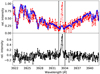 |
Fig. 2 Upper panel: comparison of the Ca K line in HD 189733 (dashed red) and HD 10476 (solid blue). Lower panel: chromospheric excess spectrum of HD 189733 after the subtraction of HD 10476. The vertical lines denote our 1.5 Å integration band. |
Parameters of template star HD 10476.
4 Results
4.1 Time series
In Fig. 1 we show the temporal evolution of the measured excess equivalent widths of the Hα, Ca infrared triplet (IRT), and Ca H&K lines; the individual IRT and H&K equivalent widths are averaged. Clearly, all three time series are correlated, which we investigate in Sect. 4.3. Livingston et al. (2007) observed a similar behavior in solar lines. In HD 189733 the amplitude of the variation is about 100 mÅ in Ca H&K, 150 mÅ in Ca IRT, and 50 mÅ in Hα. The solar variation in these lines is much smaller: 30 mÅ in Ca K, 8 mÅ in Ca 8542, and 7 mÅ in Hα (see Figs. 11 and 12 in Livingston et al. 2007).
4.2 Periodogram analysis
In the Sun, activity variations are related to spots, faculae, and other surface features, which have lifetimes ranging from several days to months (Hathaway & Choudhary 2008). Van Driel-Gesztelyi & Green (2015) conclude that bigger sunspot groups1 take longer to decay, so that larger active regions can modulate solar activity over several solar rotations.
Assuming that HD 189733 behaves similar to the Sun, an isolated activity feature causes modulation of the stellar activity indicators related to the star’s rotation phase. To account for the limited lifetimes of active regions, we split our time series into shorter subsamples. To that end, we visually investigate the best-fit sine waves and introduce a subsample where phase shifts are apparent. This procedure is repeated until the data are well reproduced by sine waves, which leads to five subsamples (see Fig. 1).
For each subsample we calculate periodograms of all three excess equivalent width time series using the algorithm given in Zechmeister & Kürster (2009). Only during the middle of the rainy season do we have too few observations for the periodogram analysis, which corresponds to sample number 4. We focus our description on the first time interval from April 28 until June 6 that visually shows a clear sinusoidal variation. The periodogram for the Hα line is shown in Fig. 3. The strongest peak is located at 12.2 ± 0.3d. This value is in good agreement with the photometric rotation period of 11.953 ± 0.009 days reported in Henry & Winn (2008). We repeated this analysis also for the Ca IRT and found an almost identical value of 12.2 ± 0.2 days.
We then repeat this analysis for subsamples 2, 3, and 5. Here the variation is less pronounced, most likely because the active region causing the strong modulation during the first subsample decayed and new active regions formed thatare more evenly distributed over different longitudes. In most cases the stellar rotation period is recovered but with a larger error bar (see Table 5). The rotation periods derived from Hα and Ca IRTare identical within the error bars. The only exception is Ca IRT in subsample 2, where the strongest peak is located at 34 days, but a slightly smaller peak also occurs at about 12 days. We note that subsample 2 was problematic due to relatively large data gaps in our time series (see Fig. 1). We omit a discussion of the Ca H&K results, because they provide the lowest S/N.
While the rotation periods agree within their error bars, this is not true for the rotation phases at T0, which we define as midnight of July 1 2017. Thus, T0 in Table 5 is the rotation phase at this date. A natural explanation is the dynamical nature of stellar active regions. Figure 1 shows that a single sine wave typically describes two to three rotation periods adequately. This would correspond to mean active region lifetimes of about 20–30 days, which is in agreement with the lifetime of large sunspot groups (Hathaway & Choudhary 2008). The phases of the different lines are mostly in agreement within the error bars, again with the exception of the second subsample of the Ca IRT series. To verify our solutions, we phase-folded the data of every subsample accounting for the phase jumps. This exhibits a clear phase-dependent modulation in the Hα excess equivalent width on the order of 50 mÅ (see Fig. 4).
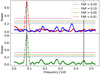 |
Fig. 3 Upper panel: periodogram of the Hα excess equivalent width based on data of subsample 1 (red). The same data, but corrected for chromospheric activity are also shown (blue). The horizontal lines denote the false alarm probabilities. The vertical lines represent the stellar rotation period and the planetary orbit period (from low to high frequency). Lower panel: identical, but for the average Ca IRT equivalent width. |
Dominant rotation periods.
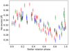 |
Fig. 4 Hα excess folded on stellar rotation period within each subsample individually. The colors of the data points are identical to the subsamples denoted in Fig. 1. |
4.3 A search for planetary Hα absorption
Our Hα time series is clearly dominated by stellar activity with an amplitude of about 50 mÅ, which strongly exceeds the planetary signal between 7 and 10 mÅ observed by Cauley et al. (2015, 2016). However, Fig. 1 shows a clear correlation between the hydrogen- and calcium-based activity indicators, which can be used to derive an activity-corrected Hα equivalent width. We base this correction on the Ca IRT lines, because they exhibit a larger S/N than the H&K lines. The analysis of Cauley et al. (2015, 2016) basically includes a first order activity correction, because the authors use the nightly out-of-transit data in the computation of the residual equivalent width. This removes stellar activity patterns over days and months so that only short-term variations over hours remain in their data.
Using the Ca IRT lines to correct the Hα time series is only valid if calcium is depleted in the upper planetary atmosphere and does not produce an absorption signal by itself. Depletion of calcium in upper planetary atmospheres has been argued by several authors, and, for example, Sing et al. (2016) show a pressure-temperature profile for HD 189733 b in combination with condensation curves of chemical species. According to their results, the atmosphere of HD 189733 is cold enough to allow for the condensation of chemical species like Ca-Ti and Al-Ca. Therefore, it is a reasonable assumption that the upper planetary atmosphere is virtually free of atomic calcium and consequently does not cause any absorption either in Ca H&K no in Ca IRT. We note, however, that this remains an assumption.
Figures 5–7 show the correlations between the Hα, Ca H&K, and Ca IRT excess equivalent widths. Although the data show a significant scatter, positive correlations are obvious between all activity indicators. Pearson’s correlation coefficient is 0.74, 0.50, and 0.51 for the three correlations with p-values of 5 × 10⁻²⁰, 2 × 10⁻⁷, and 1 × 10⁻⁷, respectively.We fit a simple linear function of the form
 (1)
(1)
and find A = 0.31 ± 0.03 and B = −36 ± 9 mÅ for the relation between Hα and Ca IRT. We then subtract the IRT-based expected Hα equivalent width from our data and call the resulting quantity the corrected Hα equivalent width. The periodogram of this value does not show any stellar rotational modulation and the remaining peaks remain below a false alarm probability of 20% (Fig. 3, blue curve). The activity correction also significantly reduces the scatter in the equivalent width values from 11.5 to 7.8 mÅ after the correction.
In Fig. 8 we plot the corrected Hα equivalent width against the planetary phase. A steady bow shock or in-transit absorption would manifest itself as systematically lower values during the corresponding phase. In contrast, we do not find any obvious phase-related variation. For a statistical analysis, we now define three samples. None of the investigations (Jensen et al. 2012; Cauley et al. 2015, 2016) found pre-transit absorption earlier than 4 h before first contact in any of their studies. Therefore, we do not expect any planetary absorption to occur more than 6 h after the end of the transit or 6 h before first contact, which we define as Sout sample. This corresponds to phases greater than +0.147 or smaller than −0.147. We further define a bow-shock sample Sbs containing in total 14 data points observed between orbital phases −0.147 and −0.034, and an in-transit sample Sin containing all data points between transit phases −0.034 and +0.034.
We use the two-sided Kolmogorov–Smirnov test to check if we can reject the null hypothesis that the samples are drawn from the same distributions. For the bow-shock sample, the test returns
 (2)
(2)
where Fi are the empirical distribution functions of the samples. The p-value is 0.18 and thus we cannot confirm that the bow-shock sample differs from the Sout sample. For the in-transit data, the Kolmogorov–Smirnov test returns D = 0.13 and p = 0.97. So far, our data provide no evidence for the existence of a bow shock or for in-transit absorption.
To further test if the means of Sbs, Sin, and Sout differ significantly and to derive upper limits, we perform a Monte Carlo analysis. We randomly chose the same number of Hα EWs (equivalent widths) as during the pre-transit phase (14 values) from the Sout sample and determine their mean for 106 draws. The resulting distribution of means is shown in Fig. 9. The mean of the Sbs sample shows a positive deflection between the 1 and 2σ interval of the distribution, which consistently provides no evidence for different parent distributions underlying Sbs and Sout. Additionally we calculated Sbs,h = 4 ± 5 mÅ and Sbs,l = 2 ± 7 mÅ, where Sbs,h is the bow-shock sample obtained during periods of high stellar activity and Sbs,l likewise but during low stellar activity. As dividing line we adopt the median activity level. Since both values are identical within their error bars, we are confident that the stellar activity level does not alter our results substantially. Ninety-nine percent of the mean values are found within ± 6.1 mÅ around the peak of the distribution. Therefore, we exclude the presence of a bow shock causing excess Hα absorption with a depth of more than 6.1 mÅ during our observing season.
We repeat the analysis for the in-transit data, finding a mean of the in-transit values of 0.8 mÅ, that is, inside the 1σ interval of the distribution from Sout. Likewise we obtain Sin,h = 0 ± 10 mÅ and Sin,l = 2 ± 4 mÅ. Again, we do not find any statistically significant dependence between the Hα flux and the stellar activity level. Here we place an upper limit of 5.6 mÅ for the maximal in-transit Hα absorption caused by the planetary atmosphere with a 99% confidence. The in-transit upper limit holds for an average absorption depth during the in-transit phases; we do not attempt to include further effects like center-to-limb variations in the stellar Hα line in the current analysis (see, e.g., Czesla et al. 2015).
We additionally investigated if data taken during high- and low-activity epochs differ significantly. We find Sout,h = −1 ± 8 mÅ and Sout,l = −1 ± 7 mÅ. This shows that also the out-of-transit data are not significantly affected by stellar activity.
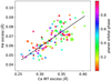 |
Fig. 5 Correlation between excess equivalent width in Hα and the average Ca IRT excess. Black line: best linear fit between the quantities. The colors of the data points correspond to the phaseangle of the planet and the sizes correspond to the error margins. |
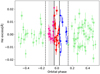 |
Fig. 8 Phase-folded, corrected Hα excess. The gray shaded area denotes a pre-transit phase of 4 h. The solid vertical lines denote the first and fourth contact. The dashed lines denote the exclusion range of 6 h before first and after the fourth contact. Observations marked with an asterisk denote epochs of high stellar activity, in which the Ca IRT excess is above median. |
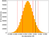 |
Fig. 9 Distribution of the results for the t-test. The black line denotes the mean of the bow-shock data points, the solid red lines denote the 1σ interval of the distribution, and the dashed red lines denote the 2σ interval. |
5 Summary and conclusions
We have collected a large, high signal-to-noise spectral dataset of HD 189733 in the observing season 2017 to search for excess Hα absorption around the transit of the hot Jupiter. Our observations randomly cover the full planetary orbit. We have determined the stellar equivalent width in theHα, Ca IRT, and Ca H&K lines and find clear evidence for stellar rotation-dominated variation. Based on the correlation between the Hα and Ca IRT equivalent widths, we derive a corrected Hα equivalent width that is free of stellar rotational modulation. In this dataset we find no evidence for the existence of a bow shock or in-transit absorption, and we place upper limits of 6.1 and 5.6 mÅ for any excess absorption during these phases with 99% confidence.
The available literature on the topic provides values of 7 and 10 mÅ bow-shock absorption and 14 mÅ in-transit absorption derived from individual transit observations (Jensen et al. 2012; Cauley et al. 2016, 2015). If calcium is indeed depleted in the upper atmosphere of HD 189733, our results exclude that such strong planetary absorption occurs on a regular basis. If the Ca IRT is absorbed in the planetary atmosphere in a similar way to the Hα line, our removal of stellar rotation-based activity variation would also remove any planetary signal. Of course, we also cannot exclude that individual transits differ from our results, for example, if strong flares or coronal mass ejections were to trigger an excited state of the planetary atmosphere. Nevertheless, our results favor the interpretation of Barnes et al. (2016), who observed that variations in the stellar Hα profile are dominated by stellar activity and that the average atmosphere of HD 189733 b causes no large Hα absorption signals.
Acknowledgements
This research has made use of the SIMBAD database and the VizieR catalog access tool, operated at CDS, Strasbourg, France, the Exoplanet Orbit Database and the Exoplanet Data Explorer at exoplanets.org, the NA SA Exoplanet Archive, which is operated by the California Institute of Technology, under contract with the National Aeronautics and Space Administration under the Exoplanet Exploration Program, PyAstronomy and NASA’s Astrophysics Data System. S.K., M.S., and S.C. acknowledge support by DFG SCHM 1032/57-1, DLR 50OR1710, BMBF 500R 1505, DFG Schm 1032/66-1, and DFG Schm 1382/2-1.
References
- Akeson, R. L., Chen, X., Ciardi, D., et al. 2013, PASP, 125, 989 [NASA ADS] [CrossRef] [Google Scholar]
- Baluev, R. V., Sokov, E. N., Shaidulin, V. S., et al. 2015, MNRAS, 450, 3101 [NASA ADS] [CrossRef] [Google Scholar]
- Barnes, J. R., Haswell, C. A., Staab, D., & Anglada-Escudé, G. 2016, MNRAS, 462, 1012 [Google Scholar]
- Boisse, I., Moutou, C., Vidal-Madjar, A., et al. 2009, A&A, 495, 959 [NASA ADS] [CrossRef] [EDP Sciences] [Google Scholar]
- Bonfanti, A., Ortolani, S., & Nascimbeni, V. 2016, A&A, 585, A5 [NASA ADS] [CrossRef] [EDP Sciences] [Google Scholar]
- Bourrier, V., Lecavelier des Etangs, A., Dupuy, H., et al. 2013, A&A, 551, A63 [NASA ADS] [CrossRef] [EDP Sciences] [Google Scholar]
- Cauley, P. W., Redfield, S., Jensen, A. G., et al. 2015, ApJ, 810, 13 [NASA ADS] [CrossRef] [Google Scholar]
- Cauley, P. W., Redfield, S., Jensen, A. G., & Barman, T. 2016, AJ, 152, 20 [NASA ADS] [CrossRef] [Google Scholar]
- Cauley, P. W., Redfield, S., & Jensen, A. G. 2017, AJ, 153, 185 [NASA ADS] [CrossRef] [Google Scholar]
- Czesla, S., Klocová, T., Khalafinejad, S., Wolter, U., & Schmitt, J. H. M. M. 2015, A&A, 582, A51 [NASA ADS] [CrossRef] [EDP Sciences] [Google Scholar]
- Ehrenreich, D., Lecavelier Des Etangs, A., Hébrard, G., et al. 2008, A&A, 483, 933 [NASA ADS] [CrossRef] [EDP Sciences] [Google Scholar]
- Ehrenreich, D., Bourrier, V., Wheatley, P. J., et al. 2015, Nature, 522, 459 [Google Scholar]
- Głȩbocki, R., & Gnaciński, P. 2005, in 13th Cambridge Workshop on Cool Stars, Stellar Systems and the Sun, eds. F. Favata, G. A. J. Hussain, & B. Battrick, ESA SP, 560, 571 [NASA ADS] [Google Scholar]
- Gray, R. O., Corbally, C. J., Garrison, R. F., et al. 2006, AJ, 132, 161 [NASA ADS] [CrossRef] [Google Scholar]
- Han, E., Wang, S. X., Wright, J. T., et al. 2014, PASP, 126, 827 [NASA ADS] [CrossRef] [Google Scholar]
- Hathaway, D. H., & Choudhary, D. P. 2008, Sol. Phys., 250, 269 [NASA ADS] [CrossRef] [Google Scholar]
- Henry, G. W., & Winn, J. N. 2008, AJ, 135, 68 [NASA ADS] [CrossRef] [Google Scholar]
- Jensen, A. G., Redfield, S., Endl, M., et al. 2012, ApJ, 751, 86 [NASA ADS] [CrossRef] [EDP Sciences] [Google Scholar]
- Kulow, J. R., France, K., Linsky, J., & Loyd, R. O. P. 2014, ApJ, 786, 132 [NASA ADS] [CrossRef] [Google Scholar]
- Lammer, H., Selsis, F., Ribas, I., et al. 2003, ApJ, 598, L121 [NASA ADS] [CrossRef] [Google Scholar]
- Lecavelier DesEtangs, A., Ehrenreich, D., Vidal-Madjar, A., et al. 2010, A&A, 514, A72 [NASA ADS] [CrossRef] [EDP Sciences] [Google Scholar]
- Livingston, W., Wallace, L., White, O. R., & Giampapa, M. S. 2007, ApJ, 657, 1137 [NASA ADS] [CrossRef] [Google Scholar]
- Martin, J., Fuhrmeister, B., Mittag, M., et al. 2017, A&A, 605, A113 [NASA ADS] [CrossRef] [EDP Sciences] [Google Scholar]
- Mittag, M., Hempelmann, A., González-Pérez, J. N., & Schmitt, J. H. M. M. 2010, Adv. Astron., 2010, 101502 [NASA ADS] [CrossRef] [Google Scholar]
- Morello, G., Waldmann, I. P., Tinetti, G., et al. 2014, ApJ, 786, 22 [NASA ADS] [CrossRef] [Google Scholar]
- Noll, S., Kausch, W., Barden, M., et al. 2013, The Cerro Paranal Advanced Sky Model [Google Scholar]
- Pace, G. 2013, A&A, 551, L8 [NASA ADS] [CrossRef] [EDP Sciences] [Google Scholar]
- Piskunov, N. E., & Valenti, J. A. 2002, A&A, 385, 1095 [NASA ADS] [CrossRef] [EDP Sciences] [Google Scholar]
- Rothman, L. S., Gordon, I. E., Barbe, A., et al. 2009, J. Quant. Spectr. Rad. Transf., 110, 533 [NASA ADS] [CrossRef] [Google Scholar]
- Salz, M., Czesla, S., Schneider, P. C., & Schmitt, J. H. M. M. 2016, A&A, 586, A75 [NASA ADS] [CrossRef] [EDP Sciences] [Google Scholar]
- Schmitt, J. H. M. M., Schröder, K.-P., Rauw, G., et al. 2014, Astron. Nachr., 335, 787 [NASA ADS] [CrossRef] [Google Scholar]
- Sing, D. K., Fortney, J. J., Nikolov, N., et al. 2016, Nature, 529, 59 [NASA ADS] [CrossRef] [Google Scholar]
- Smette, A., Sana, H., Noll, S., et al. 2015, A&A, 576, A77 [NASA ADS] [CrossRef] [EDP Sciences] [Google Scholar]
- Soubiran, C., Le Campion, J.-F., Cayrel de Strobel, G., & Caillo, A. 2010, A&A, 515, A111 [NASA ADS] [CrossRef] [EDP Sciences] [Google Scholar]
- Van Driel-Gesztelyi, L., & Green, L. M. 2015, Liv. Rev. Solar Phys., 12, 1 [Google Scholar]
- Vidal-Madjar, A., Lecavelier des Etangs, A., Désert, J.-M., et al. 2003, Nature, 422, 143 [NASA ADS] [CrossRef] [PubMed] [Google Scholar]
- Watson, A. J., Donahue, T. M., & Walker, J. C. G. 1981, Icarus, 48, 150 [NASA ADS] [CrossRef] [Google Scholar]
- Wenger, M., Ochsenbein, F., Egret, D., et al. 2000, A&AS, 143, 9 [NASA ADS] [CrossRef] [EDP Sciences] [Google Scholar]
- Zechmeister, M., & Kürster, M. 2009, A&A, 496, 577 [NASA ADS] [CrossRef] [EDP Sciences] [Google Scholar]
We are strictly speaking about the time it can be identified in magnetic field observations.
All Tables
All Figures
|
Fig. 1 Hα, Ca IRT, and Ca H&K excess equivalent width versus time. The thin black lines are the maximum power sine waves derived from our periodogram analysis and thin gray lines represent extrapolations to emphasize phase jumps. Vertical dashed lines denote the different subsamples. If the rotation period of the best-fit solution deviates significantly from the literature value of 12 days, we do not plot it. In case of Ca H&K, we removed two outliers. |
| In the text | |
|
Fig. 2 Upper panel: comparison of the Ca K line in HD 189733 (dashed red) and HD 10476 (solid blue). Lower panel: chromospheric excess spectrum of HD 189733 after the subtraction of HD 10476. The vertical lines denote our 1.5 Å integration band. |
| In the text | |
|
Fig. 3 Upper panel: periodogram of the Hα excess equivalent width based on data of subsample 1 (red). The same data, but corrected for chromospheric activity are also shown (blue). The horizontal lines denote the false alarm probabilities. The vertical lines represent the stellar rotation period and the planetary orbit period (from low to high frequency). Lower panel: identical, but for the average Ca IRT equivalent width. |
| In the text | |
|
Fig. 4 Hα excess folded on stellar rotation period within each subsample individually. The colors of the data points are identical to the subsamples denoted in Fig. 1. |
| In the text | |
|
Fig. 5 Correlation between excess equivalent width in Hα and the average Ca IRT excess. Black line: best linear fit between the quantities. The colors of the data points correspond to the phaseangle of the planet and the sizes correspond to the error margins. |
| In the text | |
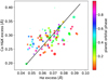 |
Fig. 6 As Fig. 5, but for Hα against Ca H&K. |
| In the text | |
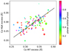 |
Fig. 7 As Fig. 5, but for Ca IRT against Ca H&K. |
| In the text | |
|
Fig. 8 Phase-folded, corrected Hα excess. The gray shaded area denotes a pre-transit phase of 4 h. The solid vertical lines denote the first and fourth contact. The dashed lines denote the exclusion range of 6 h before first and after the fourth contact. Observations marked with an asterisk denote epochs of high stellar activity, in which the Ca IRT excess is above median. |
| In the text | |
|
Fig. 9 Distribution of the results for the t-test. The black line denotes the mean of the bow-shock data points, the solid red lines denote the 1σ interval of the distribution, and the dashed red lines denote the 2σ interval. |
| In the text | |
Current usage metrics show cumulative count of Article Views (full-text article views including HTML views, PDF and ePub downloads, according to the available data) and Abstracts Views on Vision4Press platform.
Data correspond to usage on the plateform after 2015. The current usage metrics is available 48-96 hours after online publication and is updated daily on week days.
Initial download of the metrics may take a while.