| Issue |
A&A
Volume 619, November 2018
|
|
|---|---|---|
| Article Number | A115 | |
| Number of page(s) | 7 | |
| Section | Planets and planetary systems | |
| DOI | https://doi.org/10.1051/0004-6361/201833180 | |
| Published online | 13 November 2018 | |
Brown dwarf companion with a period of 4.6 yr interacting with the hot Jupiter CoRoT-20 b★
1
Observatoire Astronomique de l’Université de Genève,
51 Chemin des Maillettes,
1290
Versoix,
Switzerland
e-mail: javiera.rey@unige.ch
2
Aix Marseille Université, CNRS, Laboratoire d’Astrophysique de Marseille UMR 7326,
13388
Marseille Cedex 13,
France
3
Institut d’Astrophysique de Paris, UMR 7095 CNRS, Université Pierre & Marie Curie,
98bis boulevard Arago,
75014
Paris,
France
4
Observatoire de Haute Provence, CNRS, Aix Marseille Université,
Institut Pythéas UMS 3470,
04870
Saint-Michel-l’Observatoire,
France
5
Instituto de Astrofísica de Canarias,
C. Via Lactea s/n,
38205
La Laguna,
Tenerife,
Spain
6
Universidad de La Laguna, Departamento de Astrofísica,
38206
La Laguna,
Tenerife,
Spain
7
INAF – Osservatorio Astrofisico di Torino,
via Osservatorio 20,
10025
Pino Torinese,
Italy
8
Universidad de Buenos Aires, Facultad de Ciencias Exactas y Naturales,
Buenos Aires,
Argentina
9
CONICET – Universidad de Buenos Aires, Instituto de Astronomía y Física del Espacio (IAFE),
Buenos Aires,
Argentina
10
Department of Earth and Space Sciences, Chalmers University of Technology, Onsala Space Observatory,
439 92
Onsala,
Sweden
11
Leiden Observatory, University of Leiden,
PO Box 9513,
2300
RA Leiden,
The Netherlands
12
Thüringer Landessternwarte Tautenburg,
Sternwarte 5,
07778
Tautenburg,
Germany
13
Université Côte d’Azur, OCA, CNRS,
Nice,
France
14
CNRS, Canada-France-Hawaii Telescope Corporation,
65-1238 Mamalahoa Hwy.,
Kamuela
96743,
USA
15
Astrophysics Group, Cavendish Laboratory,
J.J. Thomson Avenue,
Cambridge
CB3 0HE,
UK
16
Instituto de Astrofísica e Ciências do Espaço, Universidade do Porto, CAUP, Rua das Estrelas,
4150-762
Porto,
Portugal
Received:
6
April
2018
Accepted:
27
June
2018
We report the discovery of an additional substellar companion in the CoRoT-20 system based on six years of HARPS and SOPHIE radial velocity follow-up. CoRoT-20 c has a minimum mass of 17 ± 1 MJup and orbits the host star in 4.59 ± 0.05 yr, with an orbital eccentricity of 0.60 ± 0.03. This is the first identified system with an eccentric hot Jupiter and an eccentric massive companion. The discovery of the latter might be an indication of the migration mechanism of the hot Jupiter, via the Lidov–Kozai effect. We explore the parameter space to determine which configurations would trigger this type of interactions.
Key words: techniques: radial velocities / stars: low-mass / stars: individual: CoRoT-20 / brown dwarfs / planetary systems / planets and satellites: dynamical evolution and stability
© ESO 2018
1 Introduction
Since the discovery of the first hot Jupiter, 51 Peg b (Mayor & Queloz 1995), the formation and evolution of short-period massive planets has been a subject of debate. They were long thought to form beyond the ice line, followed by an inward migration (Lin et al. 1996), but it has been shown recently that they can also form in situ, via core accretion (e.g., Boley et al. 2016; Batygin et al. 2016). In the first scenario, several migration processes are possible, such as disk-driven migration (Goldreich & Tremaine 1980; Lin & Papaloizou 1986; Ward 1997; Tanaka et al. 2002) or tidal migration (Fabrycky & Tremaine 2007; Wu et al. 2007; Chatterjee et al. 2008; Nagasawa et al. 2008). Fingerprints of the different mechanisms can be found in the orbital characteristics of the hot Jupiters. Those on eccentric and/or misaligned orbits are frequently presented as the result of multi-body migration mechanisms, such as the Lidov–Kozai effect (Lidov 1962; Kozai 1962; Mazeh & Shaham 1979; Eggleton & Kiseleva-Eggleton 2001; Wu & Murray 2003), gravitational scattering (Weidenschilling & Marzari 1996; Rasio & Ford 1996; Ford et al. 2001), or secular migration (Wu & Lithwick 2011). To determine how important the role of multi-body migration is in the production of hot Jupiters, a first step is to identify the perturbing body and constrain its orbital parameters. At least a dozen multiplanetary systems including a hot Jupiter and a massive companion with a fully probed orbit have been identified by radial velocity (RV) and transit surveys (e.g., Wright et al. 2009; Damasso et al. 2015; Triaud et al. 2017). Moreover, follow-up surveys have been carried out to specifically find these companions and estimate their occurrence rate. Three examples of this are the Friends of hot Jupiters survey carried out at Keck with the HIRES spectrograph (Knutson et al. 2014; Ngo et al. 2015; Piskorz et al. 2015; Ngo et al. 2016), the long-term follow-up of WASP hot Jupiters with CORALIE (Neveu-VanMalle et al. 2016), and the GAPS program with HARPS-N (Bonomo et al. 2017). The reported discoveries of an outer massive body in hot-Jupiter systems, especially those presenting high eccentricities, create ideal conditions for the Lidov–Kozai mechanism to occur. The exchange of angular momentum between the inner and outer bodies induces secular oscillations in the eccentricity and inclination of the inner planet, known as Lidov–Kozai cycles. At each phase of high eccentricity, strong tidal dissipation occurs in the inner planet when it passes through perihelion, resulting in an inward migration. As the planet approaches the star, the combined effect of tides in the star, its oblateness, and General Relativity counterbalances the Kozai cycles more efficiently, and their amplitude decreases toward the highest value of the eccentricity. Ultimately, these oscillations are annihilated. At that time, the planet will circularize under the action of tidal effects, and its semi-major axis will decrease at a higher rate (see Fig. 1 from Wu & Murray 2003).
However, it is not evident if the identified companions actually play the role of perturbing the hot Jupiter. Knutson et al. (2014) did not find any statistically significant difference between the frequency of additional companions in systems with a circular and well-aligned hot-Jupiter orbit and eccentric and/or misaligned orbits. Other studies suggest that misalignments could also be primordial (Thies et al. 2011; Spalding & Batygin 2015), meaning that inclined hot Jupiters could also arise via disk-driven migration. Moreover, a statistical study performed on a sample of six hot Jupiters orbiting cool stars, with measured obliquities and with identified outer companions (Becker et al. 2017), showed that these outer companions should typically orbit within 20°–30° of the plane that contains the hot Jupiter, suggesting that not many systems have the necessary architecture for processes such as Kozai–Lidovto operate. Therefore, it is important to know not only which fraction of hot Jupiters have a massive companion, but also which fraction of these companions is capable of triggering the migration.
CoRoT-20 is one of the planetary systems discovered by the CoRoT space mission (Baglin et al. 2009; Moutou et al. 2013). This system is composed of a 14.7-magnitude G-type star hosting a transiting giant planet with very high density, CoRoT-20b (Deleuil et al. 2012), in an eccentric orbit with a period of 9.24 days. It was identified thanks to three CoRoT photometric transits, and characterized with 15 RV measurements using the HARPS, FIES, and SOPHIE spectrographs. Based on six years of additional observations obtained with the HARPS and SOPHIE spectrographs, we here report a new substellar companion orbiting CoRoT-20. This system is the first to be identified to have an eccentric hot Jupiter (e ≥ 0.2) and an eccentric massive companion with a fully probed orbit. It therefore represents an excellent candidate to test tidal migration models. Because the mutual inclination of the two companions is unknown, we explore the parameter space to provide possible configurations that trigger the migration via Lidov–Kozai effect.
2 Spectroscopic follow-up
A long-term RV monitoring of CoRoT-20 was made with the HARPS spectrograph (Mayor et al. 2003) from November 2011 to September 2013 and with the SOPHIE spectrograph (Perruchot et al. 2008; Bouchy et al. 2009a) from October 2013 to November 2017. A total of 33 new RV measurements spanning six years were obtained and are listed in Table 1. Previous observations were obtained between December 2010 and January 2011 and are described in the discovery paper of CoRoT-20b (Deleuil et al. 2012). They are also included in our analysis. The HARPS observing mode was exactly the same as described in Deleuil et al. (2012).
The SOPHIE spectroscopic observations were made using the slow reading mode of the detector and high-efficiency (HE) objAB mode of the spectrograph, providing a spectral resolution of 39 000 at 550 nm, and where fiber B is used to monitor the sky background. The online data reduction pipeline was used to extract the spectra. The signal-to-noise ratio (S/N) per pixel at 550 nm, obtained in 1 h exposure, is between 11 and 24. The RVs were derived by cross-correlating spectra with a numerical G2V mask (Baranne et al. 1996; Pepe et al. 2002). We also derived the FWHM, contrast, and bisector span of the cross-correlation function (CCF) as described by Queloz et al. (2001). Some measurements contaminated by the Moon (flagged in Table 1) were corrected following the procedure described by Bonomo et al. (2010). The charge transfer inefficiency (CTI) of the SOPHIE CCD, a systematic effect that affects the RVs at low S/N (Bouchy et al. 2009b), was also corrected following the empirical function described by Santerne et al. (2012). Finally, the long-term instrumental instability was monitored through the systematic observation in HE modeof the RV standard stars HD185144 and HD9407, which are known to be stable at the level of a few ms−1 (Bouchy et al. 2013). We interpolated the RV variations of these standards and used it to correct our measurements following the procedure described by Courcol et al. (2015). When no correction was possible, we quadratically added 13 ms−1 to the uncertainties, which corresponds to the dispersion of the RV standard stars in HE mode (Santerne et al. 2016). Two SOPHIE spectra taken on 2013 March 25 and 26 were removed from our analysis because their S/N was very low and they were strongly contaminated by the full Moon.
Log of additional RV observations.
3 Analysis and results
3.1 Orbit fitting with DACE
For the orbital fitting and parameter determination, we used the Data and Analysis Center for Exoplanets (DACE1). DACE is a web platform dedicated to exoplanet data visualization and analysis. In particular, its tools for RV analysis allowed us to fit a preliminary solution using the periodogram of our RVs. The analytical method used to estimate these parameters is described in Delisle et al. (2016). We used this approach to fit a two-Keplerian model to the SOPHIE, HARPS, and FIES data. For the hot-Jupiter solution, the period and primary transit epoch were fixed to the values derived from the photometric analysis of Deleuil et al. (2012), which are listed in Table 2. All other parameters (nine orbital parameters and the instrumental offsets) were let free. The results of this preliminary solution were used as uniform priors for a Markov chain Monte Carlo (MCMC) analysis, also available on DACE. The algorithm used for the MCMC is described in Díaz et al. (2014, 2016). The derived median parameters of the orbital solution are listed in Table 2. The error bars represent the 68.3% confidence intervals.
Stellar and orbital parameters.
3.2 System parameters
Our long-term RV follow-up reveals an additional companion in the system, with a minimum mass of m sin i = 17 MJup, orbiting the star on an eccentric orbit of 4.6 yr. The best-fit orbit, residuals, and periodogram of the residuals are shown in Fig. 1. Additionally, the phase-folded RVs are shown in Fig. 2. It is noteworthy that the eccentricities and periastron arguments of the two orbiting companions are both very similar. No correlations were found between the velocities and the CCF parameters, which might indicate stellar activity or a blend with a stellar companion. Moreover, the photometricanalysis of Deleuil et al. (2012) indicates that CoRoT-20 is a quiet star. No additional signals were found in the RV residuals. The parameters of CoRoT-20b are in agreement and within the error bars with those published by Deleuil et al. (2012). Even though more RVs were added, there was no significant improvement in the precision of the hot-Jupiter parameters. This is expected since we included an additional orbit in our fit. To estimate the detection limits, we injected planets on circular orbits at different periods and phases into our RV residuals. These fake planets were considered detectable when the false-alarm probability in the periodogram was equal to or lower than 1%. The detection limits, shown in Fig. 3, allow us to exclude companions of 1 MJup on orbits of up to 100 days, and companions more massive than 10 MJup on orbits of up to 10 000 days (9.4 AU). CoRoT-20 was also part of the sample observed by Evans et al. (2016) using lucky imaging at the Danish 1.54 m telescope in La Silla. No physically associated stellar companions were found within 6′′.
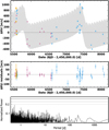 |
Fig. 1 Radial velocity curve (top panel) and residuals (middle panel) of CoRoT-20 from FIES (orange), HARPS (purple), and SOPHIE (blue). Generalized Lomb–Scargle periodogram (bottom panel) of the RVs after subtraction of the two orbits. False-alarm probability levels are plotted for 50%, 10%, and 1%. |
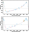 |
Fig. 2 Phase-folded RVs of CoRoT-20 b (top panel) and CoRoT-20 c (bottom panel). |
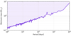 |
Fig. 3 Mean mass limit detection of a third body on a circular orbit as a function of period, based on current RV data residuals of CoRoT-20 after removing the two identified companions. We exclude the presence of any companions on circular orbits in the light blue region. |
4 Dynamical analysis with GENGA
We performed numerical simulations using the GENGA integrator (Grimm & Stadel 2014). The initial orbital parameters of both companions were taken from the best-fit values (maximum likelihood solution) of the MCMC analysis. The observations do not constrain the inclination of the outer body ic (defined in the same way asib, i.e., an orbit inclined of 90° has its plane parallel to the line of sight), nor the relative longitude of the ascending nodes of the two bodies (Δ Ω ≡ Ωb –Ωc), which has a dynamical influence. We thus explored these parameters on a 40 × 40 grid covering a large part of their domains (ic ∈ [5°;175°] knowing that values near 0° and 180° are unstablebecause of perpendicular orbits between CoRoT-20 b and c, with an extremely high mass of the latter; Δ Ω ∈ [0°;360°]). The known parameters were held fixed at their best-fit value over the grid (see Table 2), except for the mass of the outer companion Mc. This was adjusted in accordance with ic, Mc sinic being fixed by the RV observations. Each simulation was integrated over 105 yr with a time step of 0.02 day, which is convenient with the perihelion passage of CoRoT-20 b. General Relativity effects were included. In Fig. 4, we plot the results from the 1600 simulations as the maximum amplitude of the eccentricity oscillations of the inner planet. To this grid, we superimposed curves of a fixed initial mutual inclination Im between CoRoT-20 b and c. The latteris defined as cosIm = cosib cosic + cosΔΩ sinib sinic, and therefore Im ∈ [0°;180°]. The dashed and dash-dotted curves delimit zones outside of which the mutual inclination is compatible with the appearance of Kozai cycles (Im ∈ [39°, 141°]). Strictly speaking, the critical values of 39° and 141° apply to the case of a circular external orbit and a massless inner body. However, these limits provide an adequate level of precision for a qualitative reasoning. Figure 4 shows that such cycles might occur in the system. Based on analytical calculations from Fabrycky & Tremaine (2007) and Matsumura et al. (2010), we find that the Kozai effect is stronger in the CoRoT-20 system than General Relativity and tides. The timescales of the inner body’s precession of argument of periastron are the following: due to the Kozai effect, τK ~ 2.3 × 10³ yr ~ 8.9 × 10⁴ Pb; for General Relativity, τGR ~ 4.2 × 10⁴ yr ~ 1.7 × 10⁶ Pb; and for tides, τtides ~ 3.6 105 yr ~ 14.3 × 10⁶ Pb. The estimate for tides takes into account both the love numbers of the star and the inner planet. Arbitrary values for these were found in Table 1 from Wu & Murray (2003).
The largest Kozai cycles are located in the red zones, where the amplitude of the eccentricity oscillations is the most significant. To illustrate this, Fig. 5 shows the temporal evolution of the eccentricity of the inner planet for two different initial conditions corresponding to the red and blue regions of Fig. 4 (the red and blue curves, respectively). The purple dashed curve indicates the evolution of the mutual inclination associated to the same initial conditions as the red curve. Both lines being phase opposed, it clearly depicts an alternation between high eccentricity of the inner body and high mutual inclination, which is characteristic of Kozai cycles. Furthermore, the four small regions of low-eccentricity variation of the inner planet from Fig. 4 (two located at ic ~40°, and two at ic ~ 140°) are compatible with the Lidov–Kozai effect as well. These zones surround fixed points of high eccentricity and high mutualinclination of the phase space, as shown in Fig. 6. In this figure, the variation of the argument ofperiastron of the inner planet is calculated in the external body’s frame for each initial condition. The same small libration zones as in Fig. 4 are observed, depicting an oscillation of both eb and ωb∕ref c as expected nearby the Kozai fixed points (see Fig. 5 from Kozai 1962). By further comparing Figs. 4 and 6, we note that the red boxes of Fig. 4 are located in the circulation regime of ωb∕ref c. The corresponding Kozai cycles are thus qualified as rotating, while the small blue regions consist of librating type cycles.
The white zones in Figs. 4 and 6 correspond to unstable regions of the parameter space, either because the inner planet collided with the star (too high eccentricity) or because of a real instability (collision with the outer body, or ejection). We thereby exclude the corresponding doublets of parameters (ic, Δ Ω). These sets maximize the mutual inclination Im, that is, they are associated with Im ~ 90° and Im ~ 270° (the isocurve of which is phase opposed to the former). However, we recall that only the initial parameters ic, Mc, and Δ Ω were varied along the grid. All the others were fixed at their maximum likelihood value. If we had changed them along the grid according to their posterior distributions, the results would probably have been slightly different as we would have explored different regions of the phase space.
The observations show a rather good alignment of the arguments of periastron (the best-fit values exhibit |ωb − ωc|~ 8°). The nature of this alignment, coincidence or hidden dynamical process, could add constraints on the history of the system. We considered the temporal evolution of this alignment in our simulations. In the observer’s frame, ωb − ωc librates in the non-coplanar regions of the grid, and it circulates elsewhere. The pattern is similar to Fig. 6, except that the libration zones have a larger amplitude of between 80° and 120°. The oscillations of ωb − ωc indicate the existence of a dynamical process. The latter is naturally identified as Kozai cycles of librating type, as they impose an oscillation of ωb while ωc is nearly constant over time. Indeed, CoRoT-20 c is at least four times more massive than CoRoT-20 b, and their period ratio is Pc ∕Pb ~ 180. Most of the angular momentum of the system therefore comes from the outer body and the orbit of the latter is nearly purely Keplerian. However, because the amplitude of the oscillations of ωb − ωc is large, we investigated their significance. We found that in the libration zones, the arguments of periastron spend approximately twice as much time aligned (|ωb− ωc|≤ 10°) than in the circulation regions, thatis, about 12% against 6%. These proportions are valid for the beginning of the simulations. For some initial conditions, a slow increase of |ωb − ωc| is superimposed to the oscillations, so that in the end, only a small temporal fraction is spent in the alignment configuration. We thus interpret the similarity between ωb and ωc as a coincidence, with a probability of approximately 12% for observing it if the Lidov–Kozai effect is active. The latter does not maintain a permanent alignment between the arguments of periastron of both bodies because the oscillations of ωb are too large in the observer’s frame and the process does not lock ωc at a fixed value.
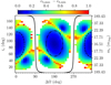 |
Fig. 4 Difference between the maximum and minimum eccentricities of the inner planet over the whole simulation for each set (ic, Δ Ω). White squares represent aborted simulations (collision or ejection of one body). The black lines are isocurves of Im, the mutual inclination. The solid line corresponds to Im = 90°, the dashed line to Im = 39°, and the dash-dotted line to Im = 141°. |
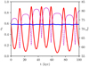 |
Fig. 5 Temporal evolution of the eccentricity of the inner planet from initial conditions in both red and blue zones of Fig. 4 (red and blue curves, respectively). The red curve corresponds to the values (ic, ΔΩ) = (70.4°, 72°) and an initial mutual inclination of Im = 72.5°. The evolution of the latter with time is represented by the dashed purple curve. The blue curve is associated with the initial set (ic, Δ Ω) = (44.2°, 144°) and Im = 122.8°. Its variationwith time is negligible. |
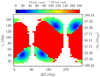 |
Fig. 6 Amplitude of the variations of the argument of periastron of the inner planet ωb∕ref c, computed in the external body’s reference frame for every initial set (ic, Δ Ω). An amplitude of 180° corresponds to a circulation of ωb∕ref c. Zones of libration exist for initially non-coplanar configurations. These regions are identical to the low-amplitude high-eccentricity zones of Fig. 4. |
5 Discussion
In single-planet systems, the circumstellar disk can induce moderate eccentricities on the body (e.g. Rosotti et al. 2017; Teyssandier & Ogilvie 2017). In multi-planet systems, however, the disk damps the eccentricities raised by the gravitational interactions between the different planets. The currently high eccentricity of CoRoT-20 b is therefore expected to be entirely due to the presence of CoRoT-20 c. There are at least three migration mechanisms that can explain the existence of close-in hot-Jupiters on eccentric orbits. The Lidov–Kozai mechanism is one of them and was studied in the previous section. Another scenario is gravitational scattering. In this process, three or more massive bodies form around the central star and move on unstable orbits. As a result of close encounters, one of the bodies is ejected from the system, leaving the remaining planets on eccentric orbits. However, such a process hardly explains the existence of planets as close to the central star as CoRoT-20 b. The third mechanism is secular migration. In this scenario, a system composed of two or more well-spaced, eccentric, and inclined planets with chaotic initial conditions will present an evolution that can lead to the existence of an eccentric hot Jupiter. Nevertheless, if such a process was taking place, we would expect the orbit of CoRoT-20 c to have evolved toward zero eccentricity (Wu & Lithwick 2011). Nagasawa et al. (2008) have explored the possibility of a coupling between these different mechanisms. Finally, Almenara et al. (2018) have recently discussed an alternative migration mechanism to explain eccentric hot Jupiters, based on interactions between two planets at low relative inclination. However, for this mechanism to work, it requires an oscillation of the angle ϖb − ϖc over time, where ϖ denotes the longitude of periastron (ϖ = Ω + ω). In other words, the coplanar system has to be located close to the high-eccentricity fixed point of the phase space; see Fig. 12 in Almenara et al. (2018). This is incompatible with our simulations, which show a circulation of ϖb - ϖc for ib ~ ic. Considering the system as described in this work, that is, with two detected companions, the Lidov–Kozai mechanism seems to be the most likely and simplest scenario to explain the current configuration. Wang et al. (2017) very recently have further consolidated this conclusion. They asserted that the Lidov–Kozai mechanism has the highest efficiency in producing hot Jupiters on eccentric orbits. The results of our numerical simulations give some constraints on the unknown parameters Δ Ω and ic. Based on the uncertainties on ic, we derived the range of possible values for Mc. We find that Mc is in the range 16.5–69.6 MJup, placing CoRoT-20 c in the domain of brown dwarfs.
Inferences about the formation of the system are highly speculative. However, our conclusions may initiate further investigations. We assert that the Lidov–Kozai migration may play a role in the actual state of CoRoT-20 b. If this is confirmed (by better constraints on ic, Mc, or Δ Ω), it would implyan outward formation of the planet followed by said migration. Nevertheless, this is not incompatible with a formation relatively close to the star, that is, inside the ice line, and at a low eccentricity. The high density of the planet, 8.87± 1.10 g cm−3 according toDeleuil et al. (2012), might be a clue to further study its formation. The high mass of the external body may be the result of a star-like formation, that is, by gravitational collapse of a primordial nebula. The high eccentricity and perhaps high inclination observed would naturally result from this process as long as the circumstellar disk that existed around CoRoT-20 was sufficiently diffuse or short-lived to keep high values of these parameters. A measure of the spin-orbit misalignment between the star and theorbit of CoRoT-20 b via the Rossiter–McLaughlin effect could clarify the value of the inclination of CoRoT-20 c (e.g., Batygin 2012; Zanazzi & Lai 2018). The age of the star is currently poorly constrained (T ∈ [60;900] Myr). Reducing this uncertainty might yield a clue in the formation process as well.
Complementary observational techniques might help constrain the mass of the second companion. We estimated the expected transit-timing variations (TTVs) of CoRoT-20b by performing the same photodynamical modeling as in Almenara et al. (2018). We modeledthe three transits observed with CoRoT (Deleuil et al. 2012), and the RV measurements from the HARPS, FIES, and SOPHIE spectrographs. We used normal priors for the stellar mass and radius from Deleuil et al. (2012), and non-informative uniform prior distributions were used for the remaining parameters. The posterior TTVs of CoRoT-20b are plotted in Fig. 7. They have the periodicity of CoRoT-20c, and an amplitude <5 min at a 68% credible interval. Furthermore, with this approach we can constrain the orbital inclination of CoRoT-20c to the range ![$[7, 172]^{o}$](/articles/aa/full_html/2018/11/aa33180-18/aa33180-18-eq1.png) at the 95% highest density interval, and its mass to 28
at the 95% highest density interval, and its mass to 28 MJ (68% credible interval).
The Gaia astrometric mission (Gaia Collaboration 2016) will have a microarcsecond precision and a maximum of sensitivity close to the period of CoRoT-20 c. We expect an astrometric signature of at least α ~33.6 μas. With a total of 63 expected observations (from the Gaia Observation Forecast Tool) and according to the magnitude of CoRoT-20, a final S/N of at least 3.8 would be obtained at the end of the mission. A combined analysis of RV and astrometry would be challenging, but it might help constrain the inclination and mass of the second body as well as the longitude of the ascending node. Finally, if the system is close to coplanar, the second companion would have some probabilitiesto transit in mid-November 2020, but with an uncertainty of about one month. Assuming a radius of 0.8 RJup, the transit depth will be 6 mmag with a duration of up to 12 h. This transit may be detectable from dedicated ground-based photometricsurveys such as NGTS (Wheatley et al. 2018). When we examined the data for previous transits (mid-October 2011 and end of March 2007), we found that the CoRoT observations of this system, obtained between 1 March and 25 March 2010, could not have covered it. Measuring the stellar obliquity with the inner planet CoROT-20 b through the Rossiter–McLaughlin effect would provide additional constraints, as stated above. As explained inDeleuil et al. (2012), the expected amplitude of the RV anomaly of the Rossiter–McLaughlin effect (22 ± 5 m s−1) is too small to be detected with HARPS according to the typical photon-noise uncertainty (20–30 m s−1), but it can be easily measured with ESPRESSO on the Very Large Telescope (Pepe et al. 2014).
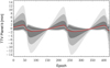 |
Fig. 7 Posterior TTVs of CoRoT-20b from the photodynamical modeling of the system. One thousand random draws from the posterior distribution are used to estimate the TTVs after the subtraction of linear ephemerides for each posterior sample. Thethree different gray regions represent the 68.3%, 95.5%, and 99.7% credible intervals, the white line is the median value of the distribution, and the red line correspond to the TTVs of the maximum a posteriori model. The TTV amplitude is shown versus the CoRoT-20 b epoch number (0 is the first transit observed by CoRoT), up to the end of 2020. |
Acknowledgements
We gratefully acknowledge the Programme National de Planétologie (telescope time attribution and financial support) of CNRS/INSU and the Swiss National Science Foundation for their support. We warmly thank the OHP staff for their support on the 1.93 m telescope. This work has been carried out in the frame of the National Centre for Competence in Research “PlanetS” supported by the Swiss National Science Foundation (SNSF). J.R. acknowledges support from CONICYT-Becas Chile (Grant No. 72140583). S.C.C.B. acknowledges support from Fundaçāo para a Ciência e a Tecnologia (FCT) through national funds and by FEDER through COMPETE2020 by these grants UID/FIS/04434/2013 & POCI-01-0145-FEDER-007672 and PTDC/FIS-AST/1526/2014 & POCI-01-0145-FEDER-016886; and also acknowledges support from FCT through Investigador FCT contracts IF/01312/2014/CP1215/CT0004. Finally, we thank the referee for their thorough review and highly appreciate the comments and suggestions, which contributed to improving this publication.
References
- Almenara, J. M., Díaz, R. F., Hébrard, G., et al. 2018, A&A, 615, A90 [NASA ADS] [CrossRef] [EDP Sciences] [Google Scholar]
- Baglin, A., Auvergne, M., Barge, P., et al. 2009, in Transiting Planets, ed. F. Pont, D. Sasselov, & M. J. Holman, IAU Symp., 253, 71 [NASA ADS] [CrossRef] [Google Scholar]
- Baranne, A., Queloz, D., Mayor, M., et al. 1996, A&AS, 119, 373 [NASA ADS] [CrossRef] [EDP Sciences] [Google Scholar]
- Batygin, K. 2012, Nature, 491, 418 [NASA ADS] [CrossRef] [PubMed] [Google Scholar]
- Batygin, K., Bodenheimer, P. H., & Laughlin, G. P. 2016, ApJ, 829, 114 [NASA ADS] [CrossRef] [Google Scholar]
- Becker, J. C., Vanderburg, A., Adams, F. C., Khain, T., & Bryan, M. 2017, AJ, 154, 230 [NASA ADS] [CrossRef] [Google Scholar]
- Boley, A. C., Granados Contreras, A. P., & Gladman, B. 2016, ApJ, 817, L17 [NASA ADS] [CrossRef] [Google Scholar]
- Bonomo, A. S., Santerne, A., Alonso, R., et al. 2010, A&A, 520, A65 [NASA ADS] [CrossRef] [EDP Sciences] [Google Scholar]
- Bonomo, A. S., Desidera, S., Benatti, S., et al. 2017, A&A, 602, A107 [NASA ADS] [CrossRef] [EDP Sciences] [Google Scholar]
- Bouchy, F., Hébrard, G., Udry, S., et al. 2009a, A&A, 505, 853 [NASA ADS] [CrossRef] [EDP Sciences] [Google Scholar]
- Bouchy, F., Isambert, J., Lovis, C., et al. 2009b, EAS Pub. Ser., 37, 247 [NASA ADS] [CrossRef] [EDP Sciences] [Google Scholar]
- Bouchy, F., Díaz, R. F., Hébrard, G., et al. 2013, A&A, 549, A49 [NASA ADS] [CrossRef] [EDP Sciences] [Google Scholar]
- Chatterjee, S., Ford, E. B., Matsumura, S., & Rasio, F. A. 2008, ApJ, 686, 580 [NASA ADS] [CrossRef] [Google Scholar]
- Courcol, B., Bouchy, F., Pepe, F., et al. 2015, A&A, 581, A38 [NASA ADS] [CrossRef] [EDP Sciences] [Google Scholar]
- Damasso, M., Esposito, M., Nascimbeni, V., et al. 2015, A&A, 581, L6 [NASA ADS] [CrossRef] [EDP Sciences] [Google Scholar]
- Deleuil, M., Bonomo, A. S., Ferraz-Mello, S., et al. 2012, A&A, 538, A145 [NASA ADS] [CrossRef] [EDP Sciences] [Google Scholar]
- Delisle, J.-B., Ségransan, D., Buchschacher, N., & Alesina, F. 2016, A&A, 590, A134 [NASA ADS] [CrossRef] [EDP Sciences] [Google Scholar]
- Díaz, R. F., Almenara, J. M., Santerne, A., et al. 2014, MNRAS, 441, 983 [NASA ADS] [CrossRef] [Google Scholar]
- Díaz, R. F., Ségransan, D., Udry, S., et al. 2016, A&A, 585, A134 [NASA ADS] [CrossRef] [EDP Sciences] [Google Scholar]
- Eggleton, P. P., & Kiseleva-Eggleton, L. 2001, ApJ, 562, 1012 [NASA ADS] [CrossRef] [Google Scholar]
- Evans, D. F., Southworth, J., Maxted, P. F. L., et al. 2016, A&A, 589, A58 [NASA ADS] [CrossRef] [EDP Sciences] [Google Scholar]
- Fabrycky, D., & Tremaine, S. 2007, ApJ, 669, 1298 [NASA ADS] [CrossRef] [Google Scholar]
- Ford, E. B., Havlickova, M., & Rasio, F. A. 2001, Icarus, 150, 303 [NASA ADS] [CrossRef] [Google Scholar]
- Gaia Collaboration (Brown, A. G. A., et al.) 2016, A&A, 595, A2 [NASA ADS] [CrossRef] [EDP Sciences] [Google Scholar]
- Goldreich, P., & Tremaine, S. 1980, ApJ, 241, 425 [NASA ADS] [CrossRef] [MathSciNet] [Google Scholar]
- Grimm, S. L.,& Stadel, J. G. 2014, ApJ, 796, 23 [NASA ADS] [CrossRef] [Google Scholar]
- Knutson, H. A., Fulton, B. J., Montet, B. T., et al. 2014, ApJ, 785, 126 [NASA ADS] [CrossRef] [Google Scholar]
- Kozai, Y. 1962, AJ, 67, 591 [Google Scholar]
- Lidov, M. L. 1962, Planet. Space Sci., 9, 719 [NASA ADS] [CrossRef] [Google Scholar]
- Lin, D. N. C., & Papaloizou, J. 1986, ApJ, 309, 846 [NASA ADS] [CrossRef] [Google Scholar]
- Lin, D. N. C., Bodenheimer, P., & Richardson, D. C. 1996, Nature, 380, 606 [NASA ADS] [CrossRef] [Google Scholar]
- Matsumura, S., Peale, S. J., & Rasio, F. A. 2010, ApJ, 725, 1995 [NASA ADS] [CrossRef] [Google Scholar]
- Mayor, M., & Queloz, D. 1995, Nature, 378, 355 [NASA ADS] [CrossRef] [Google Scholar]
- Mayor, M., Pepe, F., Queloz, D., et al. 2003, Messenger, 114, 20 [Google Scholar]
- Mazeh, T., & Shaham, J. 1979, A&A, 77, 145 [Google Scholar]
- Moutou, C., Deleuil, M., Guillot, T., et al. 2013, Icarus, 226, 1625 [NASA ADS] [CrossRef] [Google Scholar]
- Nagasawa, M., Ida, S., & Bessho, T. 2008, ApJ, 678, 498 [NASA ADS] [CrossRef] [Google Scholar]
- Neveu-VanMalle, M., Queloz, D., Anderson, D. R., et al. 2016, A&A, 586, A93 [NASA ADS] [CrossRef] [EDP Sciences] [Google Scholar]
- Ngo, H., Knutson, H. A., Hinkley, S., et al. 2015, ApJ, 800, 138 [NASA ADS] [CrossRef] [Google Scholar]
- Ngo, H., Knutson, H. A., Hinkley, S., et al. 2016, ApJ, 827, 8 [NASA ADS] [CrossRef] [Google Scholar]
- Pepe, F., Mayor, M., Galland, F., et al. 2002, A&A, 388, 632 [NASA ADS] [CrossRef] [EDP Sciences] [Google Scholar]
- Pepe, F., Molaro, P., Cristiani, S., et al. 2014, Astron. Nachr., 335, 8 [NASA ADS] [CrossRef] [Google Scholar]
- Perruchot, S., Kohler, D., Bouchy, F., et al. 2008, in Ground-based and Airborne Instrumentation for Astronomy II, Proc. SPIE, 7014, 70140J [CrossRef] [Google Scholar]
- Piskorz, D., Knutson, H. A., Ngo, H., et al. 2015, ApJ, 814, 148 [NASA ADS] [CrossRef] [Google Scholar]
- Queloz, D., Henry, G. W., Sivan, J. P., et al. 2001, A&A, 379, 279 [NASA ADS] [CrossRef] [EDP Sciences] [Google Scholar]
- Rasio, F. A., & Ford, E. B. 1996, Science, 274, 954 [NASA ADS] [CrossRef] [PubMed] [Google Scholar]
- Rosotti, G. P., Booth, R. A., Clarke, C. J., et al. 2017, MNRAS, 464, L114 [NASA ADS] [CrossRef] [Google Scholar]
- Santerne, A., Díaz, R. F., Moutou, C., et al. 2012, A&A, 545, A76 [NASA ADS] [CrossRef] [EDP Sciences] [Google Scholar]
- Santerne, A., Moutou, C., Tsantaki, M., et al. 2016, A&A, 587, A64 [NASA ADS] [CrossRef] [EDP Sciences] [Google Scholar]
- Spalding, C., & Batygin, K. 2015, ApJ, 811, 82 [NASA ADS] [CrossRef] [Google Scholar]
- Tanaka, H., Takeuchi, T., & Ward, W. R. 2002, ApJ, 565, 1257 [NASA ADS] [CrossRef] [Google Scholar]
- Teyssandier, J., & Ogilvie, G. I. 2017, MNRAS, 467, 4577 [NASA ADS] [CrossRef] [Google Scholar]
- Thies, I., Kroupa, P., Goodwin, S. P., Stamatellos, D., & Whitworth, A. P. 2011, MNRAS, 417, 1817 [NASA ADS] [CrossRef] [Google Scholar]
- Triaud, A. H. M. J., Neveu-VanMalle, M., Lendl, M., et al. 2017, MNRAS, 467, 1714 [NASA ADS] [Google Scholar]
- Wang, Y., Zhou, J.-l., Hui-gen, L., & Meng, Z. 2017, ApJ, 848, 1 [Google Scholar]
- Ward, W. R. 1997, Icarus, 126, 261 [NASA ADS] [CrossRef] [Google Scholar]
- Weidenschilling, S. J., & Marzari, F. 1996, Nature, 384, 619 [NASA ADS] [CrossRef] [PubMed] [Google Scholar]
- Wheatley, P. J., West, R. G., Goad, M. R., et al. 2018, MNRAS, 475, 4476 [NASA ADS] [CrossRef] [Google Scholar]
- Wright, J. T., Upadhyay, S., Marcy, G. W., et al. 2009, ApJ, 693, 1084 [NASA ADS] [CrossRef] [Google Scholar]
- Wu, Y., & Lithwick, Y. 2011, ApJ, 735, 109 [NASA ADS] [CrossRef] [Google Scholar]
- Wu, Y., & Murray, N. 2003, ApJ, 589, 605 [NASA ADS] [CrossRef] [EDP Sciences] [Google Scholar]
- Wu, Y., Murray, N. W., & Ramsahai, J. M. 2007, ApJ, 670, 820 [NASA ADS] [CrossRef] [Google Scholar]
- Zanazzi, J. J.,& Lai, D. 2018, MNRAS, 478, 835 [NASA ADS] [CrossRef] [Google Scholar]
The DACE platform developed by the National Center of Competence in Research PlanetS is available at http://dace.unige.ch.
All Tables
All Figures
|
Fig. 1 Radial velocity curve (top panel) and residuals (middle panel) of CoRoT-20 from FIES (orange), HARPS (purple), and SOPHIE (blue). Generalized Lomb–Scargle periodogram (bottom panel) of the RVs after subtraction of the two orbits. False-alarm probability levels are plotted for 50%, 10%, and 1%. |
| In the text | |
|
Fig. 2 Phase-folded RVs of CoRoT-20 b (top panel) and CoRoT-20 c (bottom panel). |
| In the text | |
|
Fig. 3 Mean mass limit detection of a third body on a circular orbit as a function of period, based on current RV data residuals of CoRoT-20 after removing the two identified companions. We exclude the presence of any companions on circular orbits in the light blue region. |
| In the text | |
|
Fig. 4 Difference between the maximum and minimum eccentricities of the inner planet over the whole simulation for each set (ic, Δ Ω). White squares represent aborted simulations (collision or ejection of one body). The black lines are isocurves of Im, the mutual inclination. The solid line corresponds to Im = 90°, the dashed line to Im = 39°, and the dash-dotted line to Im = 141°. |
| In the text | |
|
Fig. 5 Temporal evolution of the eccentricity of the inner planet from initial conditions in both red and blue zones of Fig. 4 (red and blue curves, respectively). The red curve corresponds to the values (ic, ΔΩ) = (70.4°, 72°) and an initial mutual inclination of Im = 72.5°. The evolution of the latter with time is represented by the dashed purple curve. The blue curve is associated with the initial set (ic, Δ Ω) = (44.2°, 144°) and Im = 122.8°. Its variationwith time is negligible. |
| In the text | |
|
Fig. 6 Amplitude of the variations of the argument of periastron of the inner planet ωb∕ref c, computed in the external body’s reference frame for every initial set (ic, Δ Ω). An amplitude of 180° corresponds to a circulation of ωb∕ref c. Zones of libration exist for initially non-coplanar configurations. These regions are identical to the low-amplitude high-eccentricity zones of Fig. 4. |
| In the text | |
|
Fig. 7 Posterior TTVs of CoRoT-20b from the photodynamical modeling of the system. One thousand random draws from the posterior distribution are used to estimate the TTVs after the subtraction of linear ephemerides for each posterior sample. Thethree different gray regions represent the 68.3%, 95.5%, and 99.7% credible intervals, the white line is the median value of the distribution, and the red line correspond to the TTVs of the maximum a posteriori model. The TTV amplitude is shown versus the CoRoT-20 b epoch number (0 is the first transit observed by CoRoT), up to the end of 2020. |
| In the text | |
Current usage metrics show cumulative count of Article Views (full-text article views including HTML views, PDF and ePub downloads, according to the available data) and Abstracts Views on Vision4Press platform.
Data correspond to usage on the plateform after 2015. The current usage metrics is available 48-96 hours after online publication and is updated daily on week days.
Initial download of the metrics may take a while.