| Issue |
A&A
Volume 618, October 2018
|
|
|---|---|---|
| Article Number | A180 | |
| Number of page(s) | 21 | |
| Section | Cosmology (including clusters of galaxies) | |
| DOI | https://doi.org/10.1051/0004-6361/201833630 | |
| Published online | 30 October 2018 | |
Luminosity functions of cluster galaxies
The near-ultraviolet luminosity function at < z > ∼ 0.05
1
FINCA, University of Turku, Vesilinnantie 5, 20014 Turku, Finland
e-mail: This email address is being protected from spambots. You need JavaScript enabled to view it.
2
H. H. Wills Physics Laboratory, University of Bristol, Tyndall Avenue, BS1 8TL Bristol, UK
Received:
13
June
2018
Accepted:
27
July
2018
Abstract
We derive NUV luminosity functions for 6471 NUV detected galaxies in 28 0.02 < z < 0.08 clusters and consider their dependence on cluster properties. We consider optically red and blue galaxies and explore how their NUV LFs vary in several cluster subsamples, selected to best show the influence of environment. Our composite LF is well fit by the Schechter form with M*NUV = −18.98 ± 0.07 and α = −1.87 ± 0.03 in good agreement with values for the Coma centre and the Shapley supercluster, but with a steeper slope and brighter L* than in Virgo. The steep slope is due to the contribution of massive quiescent galaxies that are faint in the NUV. There are significant differences in the NUV LFs for clusters having low and high X-ray luminosities and for sparse and dense clusters, though none are particularly well fitted by the Schechter form, making a physical interpretation of the parameters difficult. When splitting clusters into two subsamples by X-ray luminosity, the ratio of low to high NUV luminosity galaxies is higher in the high X-ray luminosity subsample (i.e., the luminosity function is steeper across the sampled luminosity range). In subsamples split by surface density, when characterised by Schechter functions the dense clusters have an M* about a magnitude fainter than that of the sparse clusters and α is steeper (−1.9 vs. −1.6, respectively). The differences in the data appear to be driven by changes in the LF of blue (star-forming) galaxies. This appears to be related to interactions with the cluster gas. For the blue galaxies alone, the luminosity distributions indicate that for high LX and high velocity dispersion cluster subsamples (i.e., the higher mass clusters), there are relatively fewer high UV luminosity galaxies (or correspondingly a relative excess of low UV luminosity galaxies) in comparison the lower mass cluster subsamples.
Key words: galaxies: luminosity function, mass function / galaxies: clusters: general / galaxies: formation / galaxies: evolution
© ESO 2018
1. Introduction
The luminosity function (hereafter LF) of a population of galaxies characterises the end result of a series of processes involving the mass assembly, star formation and morphological evolution of these galaxies. The LF therefore provides a statistical first-order description of the properties of a population of galaxies at a given epoch and yields a test of models for galaxy formation and evolution and assembly (e.g., Henriques et al. 2015; Rodrigues et al. 2017; Mitchell et al. 2018).
LFs measured in different bandpasses measure, and are sensitive to, different mechanisms involved in galaxy evolution. As an example, infrared LFs more closely resemble stellar mass functions and can be used to determine the mass assembly history of galaxies. In contrast, the near ultraviolet (NUV) LF is instead strongly affected by star formation and its evolution (and dependence on environment) as most of the flux is produced by young stars with relatively short lifetimes (<1 Gyr), although significant NUV flux can also be produced by hot horizontal branch stars in old stellar populations. Therefore, NUV observations are expected to provide clues to the importance of environmental effects in quenching star formation, especially within the cores of galaxy clusters and other high density regions, where a variety of processes (e.g., tides, interactions, mergers, ram stripping) are believed to play an important role in controlling star formation (e.g., Boselli et al. 2014, 2016b; Taranu et al. 2014; Darvish et al. 2018).
It is only recently that panoramic images in the vacuum UV have become available from the GALEX telescope (Martin et al. 2005). Limited areas of sky were earlier observed from balloonborne telescopes or experiments flown on the Space Shuttle. GALEX has provided us with the first nearly all-sky survey in the vacuum UV bands at 1500 and 2300 Å. From this, Wyder et al. (2005) produced the first (and so far, only) field UV luminosity function, but only a few clusters have been so characterised until now. From FOCA data Andreon (1999) derived a 2000 Å LF for the Coma cluster, while Cortese et al. (2003) obtained a composite LF for Virgo, Coma and Abell 1367 (also at 2000 Å). Based on GALEX data (but excluding the centre) Cortese et al. (2008) determined the UV LFs for galaxies in the Coma cluster, including quiescent and star-forming galaxies separately. Virgo has been extensively studied in the same manner by the GUVICS collaboration (Boselli et al. 2016a), while Hammer et al. (2012) have obtained a LF for a field in Coma lying between the core and the infalling NGC4839 subgroup. Finally, Haines et al. (2011) measured a composite UV LF for five clusters within the Shapley supercluster of galaxies.
The characteristic magnitude L* is observed to vary widely between Virgo, Coma, A1367 and the composite Shapley supercluster LF. This is likely due to the relatively poor number counts for bright galaxies (which tend to be the rarer spirals, rather than the more numerous red sequence ellipticals). Boselli et al. (2016a) remark that both Coma and A1367 contain a small number of bright spirals, whose star formation rates were probably increased during infall, while such objects are not present in Virgo. However, the composite LF in the Shapley supercluster (Haines et al. 2011) is in better agreement with Coma (Cortese et al. 2008) than with Virgo and the field studied by Hammer et al. (2012). Given the small number of clusters observed so far, one cannot rule out other mechanisms, such as the degree of dynamical evolution, the presence of substructure and the growth of a bright central elliptical, but our study of a large number of clusters in this paper will allow us to examine some of these issues.
The faint end slope of the LF in Coma and A1367 by Cortese et al. (2003) reaches to MNUV ∼ −17 and has a slope of >−1.4, while the Shapley supercluster composite LF by Haines et al. (2011) has a slope α ∼ −1.5/−1.6 to MNUV = −14, in contrast to the Virgo cluster (Boselli et al. 2016a), where it is flatter (α ∼ −1.2 to MNUV = −11) and closer to the field value. The value in the Coma infall field of Hammer et al. (2012) is intermediate (α = −1.4 to MNUV = −10.5but closer to the GUVICS Virgo value. The slope of the LF may depend somewhat on the depth reached. The steep faint end may also reflect the contribution from the optically bright ellipticals which are faint in the UV. For blue galaxies, LFs in the field and clusters are very similar, and this suggests that star formation is suppressed quickly upon infall (Cortese et al. 2008) so that only very recent newcomers to the cluster environment contribute to the UV LFs, while rapidly quenched galaxies are already faint in the NUV.
Here we consider the composite NUV LF of 28 clusters at moderate redshift (0.02 < z < 0.08) with highly complete redshift coverage of members and non members - even for the faintest luminosity bins we consider (NUV0 ∼ 20−21 depending on cluster), mean completeness is above 80%. We explore the effects of environment by splitting our sample into clusters of low and high velocity dispersion as well as low and high X-ray luminosity and sparse and dense clusters. Red sequence and blue cloud galaxies are also considered separately and as a function of cluster environment. Although our data do not reach as deep as that used in previous targeted studies of individual local clusters (Virgo, Coma, Abell 1367), the significantly larger number of objects studied here allows us to better control stochastic effects from small number statistics and to explore cluster to cluster variations and therefore the effects of the broad cluster environment.
In the following section we describe the sample and analysis. Results are shown in Sect. 3 and discussed in Sect. 4. All magnitudes are in the AB system, unless otherwise noted. We assume the conventional cosmological parameters from the latest Planck results.
2. Data
Our data consist of a sample of 28 clusters at 0.02 < z < 0.08 selected from the sample originally studied by De Propris et al. (2003), plus clusters from the WINGS/OmegaWINGS dataset (Cava et al. 2009; Moretti et al. 2015, 2017; Gullieuszik et al. 2015). We selected objects with available GALEX imaging in the NUV (2300 Å) band (the number of objects in the FUV band is about 1/3 of those detected in the NUV band, and we do not treat these in the present paper, although an analysis of the FUV data is presented elsewhere in a different context). We show the basic characteristics of the clusters studied in Table 1. This shows the cluster identification, coordinates, redshift (from our work and the WINGS/OmegaWINGS dataset), velocity dispersion (also from our earlier work or as presented by WINGS/OmegaWINGS), X-ray luminosity (from the literature) and the IDs of the GALEX tiles used for our analysis.
For each cluster we retrieved the appropriate tile(s) and used the available (Kron-style) photometry (Martin et al. 2005; Morrissey et al. 2007) in the NUV to select objects. We only considered detections within each cluster’s (calculated from the formula in Carlberg et al. 1997) and with a S/N of at least 5 in the NUV band. NUV magnitudes were corrected for extinction using the values provided in NED (Schlafly & Finkbeiner 2011). However, for some clusters r200 exceeded the size of the GALEX tiles and we only consider objects in the inner 0.5° of each tile, where GALEX has full sensitivity. Our spatial coverage is comparable or greater than that obtained in prior targeted studies of nearby clusters such as Virgo, Coma and Abell 1367.
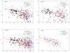 |
Fig. 1. Colour-magnitude diagrams in g − r (or BJ − RF) vs. r for NUV-selected galaxies in our clusters. Symbols as identified in the figure legends. Here we show a representative sample of objects. All remaining clusters are shown in Fig. A.1 |
GALEX has a resolution of about 5″ and it is therefore not possible to carry out star-galaxy separation from the data. For this purpose we cross-matched each of the GALEX detections with CCD images from the PanStarrs1 survey, which covers the entire sky north of δ = −30° (Chambers et al. 2016) and also provides optical photometry (Magnier et al. 2016; Flewelling et al. 2016), except for some clusters in the South where we used photographic data from the UK Schmidt Telescope SuperCosmos survey (Hambly et al. 2001b,a). For each NUV detected object we assign a star/galaxy type based on rPSF – rKron < 0.05 mag. (for a star) and direct inspection of each image with imexamine if necessary. For clusters outside of the PanStarrs footprint we instead use the star/galaxy class provided by the SuperCosmos survey, and we also check these objects visually. The matching radius was 6″, equivalent to the NUV PSF and similar to that used in previous studies. The optical photometry is also corrected for Galactic extinction from NED. We chose very conservative NUV magnitude limits, such that all our galaxies have optical counterparts, although this of course means that our LFs do not reach as faint as other work in more nearby clusters. In any case, the limiting magnitude of our study is set by the much brighter spectroscopic completeness limit, as detailed below.
We then matched (also within 6″) our galaxies with redshifts within NED (NASA extragalactic database) and other sources (such as the WINGS/OmegaWINGS catalogues in Cava et al. 2009; Gullieuszik et al. 2015; Moretti et al. 2017). Most of the redshifts come from the 2dF and SDSS surveys as well as the WINGS/OmegaWINGS survey, but a few other sources of measurements are occasionally indicated in NED.
The redshift information used comes from a variety of sources, some of which may suffer from selection effects, especially as the redshift catalogs are selected in the optical while our photometric catalog is selected in the NUV. Our analysis is based on the methods originally developed in De Propris et al. (2003) and De Propris (2017), where we correct for incompleteness based on the redshift distribution (as a function of magnitude) for field and cluster galaxies (also see Mobasher et al. 2003). In order to do this, we need to first make sure that the redshift information is not biased towards or against cluster members, as this lack of bias is an assumption of the method.
As a first step, we therefore plot the g − r vs. r colour-magnitude diagrams for all NUV-selected galaxies in Fig. 1, and fit the red sequence for each cluster using a minimum absolute deviation least squares fitting procedure (Beers et al. 1990) to remove the influence of outliers. Here we show only the first four clusters. The remaining clusters can be seen in Appendix A (with the same format). For clusters below −30° in declination, that are not in the PanStarrs footprint, we use the Supercosmos BJ − RF and RF colours instead. Note that some clusters do not have a clear colour-magnitude relation with our data, and these are not plotted in Fig. 1. Our previous work has shown that the colour dispersion about the red sequence is 0.05 mag. in g − r (De Propris 2017), in agreement with other studies (e.g., Valentinuzzi et al. 2011). We therefore exclude all objects (without a redshift) 0.15 mag. redder than the red sequence, as these are unlikely to be members. We can see from Fig. 1 that the majority of objects redder than the red sequence for which a redshift is available are non-members and the remaining galaxies with unknown redshift therefore have the same colour distribution as the sample of galaxies with known redshifts (irrespective of their being cluster members); these former objects tend to lie at the faint end of the spectroscopic sample.
In Fig. 2 we plot the equivalent of Fig. 1 but for NUV0 (i.e., the band we select galaxies in). While red sequence galaxies can be easily identified even when plotting g − r vs. NUV0, it is apparent that the optically bright red sequence galaxies are faint in NUV whereas the brighter galaxies tend to be relatively optically faint systems. For blue galaxies, NUV flux comes primarily from young stars, whereas for red galaxies UV flux is primarily provided by hot horizontal branch stars that produce the ultraviolet excess (Schombert 2016). We elaborate on this further in this paper.
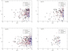 |
Fig. 2. Same as Fig. 1 but for g − r vs. NUV, with the same symbols (as indicated in the figure legend). This shows that NUV bright cluster members tend to be optically blue while the massive red sequence galaxies are generally faint in NUV. All remaining clusters are shown in Fig. A.2. |
In Fig. 3 we show the redshift completeness for all clusters as a function of NUV magnitude.
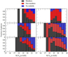 |
Fig. 3. Completeness fractions for each cluster vs. NUV0 magnitude (in the z = 0.05 bins described in the text). The numbers in the top left corner of each panel identify the cluster, in the order shown in Table 1 (here 1: Abell S1171; 2: Abell 2734; 3: EDCC 442; 4: Abell 85; 5: Abell 119; 6: Abell 168). The symbols used in the plot are identified in the figure legend. All remaining clusters are shown in Fig. A.3. |
Clusters studied in this paper.
3. The luminosity functions
We produce composite UV LFs of UV detected galaxies in the same fashion as in our previous studies of cluster optical and near-IR LFs (De Propris et al. 2003; De Propris 2017).We count galaxies in each cluster in 0.5 mag. bins shifted to their corresponding values at z = 0.05, which is the mean redshift of the sample in Table 1. For each cluster we calculate the difference in distance modulus between its redshift and z = 0.05. We then count cluster members in apparent magnitude bins corresponding to the fixed magnitude bins at z = 0.05. For instance, in Abell 1139 (cz = 11711 km s−1) the magnitude interval 14.81 < NUV0 < 15.31 contributes to the galaxy counts in the 15.25 < NUV0 < 15.75 bin at z = 0.05, whereas in Abell 2734 (cz = 18 737 km s−1) counts in the apparent magnitude bin 15.66 < NUV0 < 16.16 contribute to the equivalent 15.25 < NUV0 < 15.75 counts at z = 0.05.
In this way we avoid carrying out uncertain (and variable from galaxy to galaxy) e and k corrections to z = 0. Since only a small shift of 0.03 (maximum) in redshift is needed, the relative e + k corrections will be small. The modest error induced for clusters at z < 0.05 is compensated by an error (of the same magnitude but opposite sign) for clusters at z > 0.05 so that the composite LFs at z = 0.05 should not suffer from these uncertainties. A similar approach is used by Blanton et al. (2003) and Rudnick et al. (2009). For the assumed cosmology, the distance modulus to z = 0.05 is 36.64 mag. but this does not include the effects of e + k corrections.
In order to create a composite LF we need to correct for incompleteness. The procedure is analogous to that used in our previous work (De Propris et al. 2003; De Propris 2017). Figure 2 shows the completeness fractions as a function of observed NUV0 magnitude for all our clusters, including members, non members and objects for which no redshift is known. We then correct for incompleteness in the same manner as in De Propris et al. (2003) and Mobasher et al. (2003). We then calculate the composite LF following the procedure detailed in Colless (1989) where we generally stop the summations (for each cluster) at completeness levels of 80% or more.
Here the number of members for cluster i in each magnitude bin j is given by:
 (1)
(1)
where NI is the number of galaxies in the input photometric catalog, NM the number of cluster members and NZ the number of objects with a measured redshift (whether a cluster member or not) in each bin.
Here NI is a Poisson random variable whereas NM/NZ is a binomial variable. The mean and variance for the approximately normal distribution of the sample proportion are p and (p(1 − p)/n), where p is the probability of a “success”(i.e., a cluster member) NM/NZ and n is the number of trials NZ. Therefore the error in this quantity can be written as (ignoring a small negative second order term):
 (2)
(2)
We then calculate the composite LF following the procedure detailed in Colless (1989) where we generally stop the summations (for each cluster) at completeness levels of 80% or more.
 (3)
(3)
where Ncj is the number of cluster galaxies in magnitude bin j, and the sum is carried over the i clusters and mj is the number of clusters contributing to magnitude bin j. Here Ni0 is a normalisation factor, corresponding to the (completeness corrected) number of galaxies brighter than a given magnitude (here we use NUV0 = 19.0) in each cluster and
 (4)
(4)
The error is then given by:
![Mathematical equation: $ \begin{equation} \delta N_{cj}={N_{c0} \over m_j} \Bigg[ {\sum\limits_i} \Bigg({\delta N_{ij} \over N_{i0}}\Bigg)^2\Bigg]^{1/2}. \end{equation} $](/articles/aa/full_html/2018/10/aa33630-18/aa33630-18-eq6.gif) (5)
(5)
These summations are carried out individually and separately for each of the subsamples discussed below, so that the total numbers do not always scale between the various LFs.
3.1. Luminosity functions for all galaxies
We fit the composite NUV LF for all 28 clusters with a standard Schechter function using a Levenberg-Marquardt minimisation algorithm. This is shown in Fig. 4 together with the associated error ellipses (the LF parameters are strongly correlated). The values for M* and α are tabulated in Table 2 where we also present conditional 1σ errors for each parameter (i.e., the error holding the other parameter fixed).
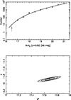 |
Fig. 4. Luminosity function and best fit for all clusters in the sample (top). Error ellipses for 1, 2 and 3σ are shown (bottom). In this and subsequent figures M* refers to the observed characteristic magnitude of the LF measured at z = 0.05. |
For all clusters the best fitting LF has  and α = −1.87 ± 0.03 (assuming the above distance modulus and no k+e correction, as noted earlier). The value we derive for this M* is in good agreement with that measured by Cortese et al. (2008) for the Coma cluster, fainter (but consistent at the ∼ 1.5σ level) than the one measured by Cortese et al. (2005) in Abell 1367 and considerably brighter than the GUVICS LF in the Virgo cluster (Boselli et al. 2016a). It is however in very good agreement with M* for the composite LF of the 5 Shapley supercluster clusters in Haines et al. (2011). The LF we derive also has a somewhat brighter M* than the local field in Wyder et al. (2005), although this latter measurement has large uncertainties (it only differs at the 1.5σ level). At face value this might indicate a brightening of the typical UV flux in cluster galaxies, possibly due to induced star formation upon first encountering the cluster enviroment. The slope is quite steep, α ∼ −1.9. This is in broad agreement with the values for α obtained for Coma, Abell 1367 and the Shapley clusters, but not with the much flatter slopes derived for the field and Virgo as well as the region in the Coma cluster studied by Hammer et al. (2012): these latter have α ∼ −1.2 to −1.4.
The differences in the bright end of the LF may be more naturally explained by small number statistics. Unlike optical LFs, the bright end of UV LFs are dominated by starforming spirals (see, e.g., Fig. 1). These objects are likely to be a transient and comparatively stochastic population that has recently become bound to the cluster (e.g., Cortese et al. 2008; Haines et al. 2011). It is therefore understandable that local conditions may drive their contribution to the bright end of the LF. Our composite LF is less sensitive to this, as it averages contributions from several clusters, spanning a wide range of properties. It is perhaps indicative that our M* is in good agreement with the composite LF of Haines et al. (2011).
The faint end of the NUV LF includes components from fainter star-forming galaxies as well as bright early-type galaxies. As these objects tend to be brighter in the UV as a function of optical luminosity (e.g., Ali et al. 2018), this leads to steeper NUV LFs in clusters (bright early-type galaxies are much rarer in the field), see below for our discussion on this. On the other hand, the LF slopes are much flatter in Virgo (Boselli et al. 2016a) and the in outskirts of Coma (Hammer et al. 2012). These authors suggest that uncertainties in completeness corrections and differences in depth (between their work and Coma/Shapley) are responsible for this effect. While our data are not as deep as those in nearby clusters, they reach ∼ 2.5 mag. below the L* point, where α should be well determined. Our completeness corrections are well understood and small (as discussed above). This may point to real differences in the faint end slope between our clusters and the regions studied by GUVICS and Hammer et al. (2012), likely due to the behaviour of faint starforming galaxies in these different environments (to which these objects should be especially sensitive). This is also further discussed in the next sections.
Schechter function parameters when fitted to full available NUV0 range for each subsample.
In order to address the above issues, we now consider the LFs of optically red and blue galaxies separately. In previous studies star-forming galaxies and quiescent galaxies were separated according to their NUV-r colour. Given the strong sensitivity of the NUV colour to star formation, this sharply separates star-forming and quenched galaxies. However, this may lead to a selection effect, as shown by Cortese et al. (2008), where recently quenched galaxies cluster on the red sequence and only currently star-forming galaxies are observed in the “blue cloud”. Because star formation is expected to be strongly suppressed in clusters, these galaxies represent a transient population of objects newly accreted from the field. This means that one observes the same blue galaxy LF in all environments, because all sensitivity to environmental effects is masked by the rapid quenching process and the sensitivity of the NUV band to star formation, although in reality the process of colour and morphological evolution is likely to be more prolonged (Bremer et al. 2018).
Here we instead select blue and red galaxies from the optical g − r colours in Fig. 1. Red sequence galaxies lie within ± 0.15 mag. (3 σ given the measured colour dispersion) of the best fitting straight line shown in Fig. 1, while our blue cloud galaxies are all objects bluer than the blue edge of the red sequence as defined above. Because the g − r colour changes more slowly after star formation declines, our choice separates galaxies into long term quiescent objects (with possibly a small fraction of galaxies showing residual star formation) and star-forming objects plus “green valley” galaxies. Our choice allows us to explore the effects of the cluster environment on star-forming galaxies on a longer timescale, closer to the crossing time of clusters and comparable to the timescale over which galaxies cross the green valley in Bremer et al. (2018).
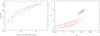 |
Fig. 5. Luminosity function and best fit for red and blue galaxies (identified by colour) for all clusters in the sample (left). Error ellipses for 1, 2 and 3σ are shown in the right-hand panel, for red and blue galaxies. |
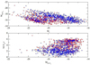 |
Fig. 6. For all galaxies in all clusters we plot the absolute magnitudes in r vs. the absolute magnitudes in NUV on the top panel. Red symbols are for red sequence galaxies and blue symbols for blue cloud galaxies. On the bottom panel we show the NUV-r colours as a function of absolute NUV magnitude. |
We plot the LFs for red and blue galaxies in Fig. 5, with the parameters tabulated in Table 2. The Schechter function is not a very good fit to the red sequence LF, however the slope is very steep. Figure 6 plots the absolute Mr vs. absolute MNUV for all galaxies, with different symbols for the optically red and blue samples. This shows that (a) red galaxies are faint in NUV and contribute mainly to the faint end of the NUV LFs, giving rise to the steep slopes (see upper panel), (b) the red galaxies are nevertheless optically bright and therefore generally more massive, being typically ∼L* or brighter in the optical (also see upper panel in this figure), whereas (c) blue galaxies are bright in NUV, but are usually optically faint (upper and lower panels of Fig. 6). Star forming galaxies in low redshift clusters are generally sub-L* systems. Figure 6 (upper panel) shows how optically bright galaxies (i.e., −20 < Mr < −22) mainly lie at −15 < MNUV < −17 i.e., they are usually 1–2 magnitudes fainter than the M* point for the NUV LF. Fainter red sequence galaxies are missing from our sample unless they are star-forming and have bluer NUV-r colours because of a selection effect. This is because the NUV-optical colour for quiescent galaxies becomes bluer with increasing luminosity as the NUV emission is produced by hot horizontal branch stars (rather than star-formation), so that we are looking at the exponential part of the galaxy mass function, as seen in the lower panel of Fig. 6. Therefore the optically bright galaxies mainly contribute to the faint end of the NUV LF and this results in a steep total LF slope. Unfortunately, no previous work seems to treat the red galaxies LF in detail, except for the study by Boselli et al. (2016a) in the Coma cluster, compared to which our M* is somewhat brighter and our α is steeper.
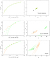 |
Fig. 7. Luminosity functions and best fits left column) and associated error ellipse (right column) for low (orange) and high (green) σ clusters (top row), low (orange) and high (green) LX clusters (middle row) and sparse (orange) and dense (green) clusters (bottom row). The circle in each figure indicates the M* and α values for the total LF. Clearly, for the subsamples split by X-ray luminosity and surface density, the luminosity distributions as sampled here are not well fitted by Schechter functions, the location and size of the error ellipses in these cases should be used with caution. Any interpretation should take note of the actual numbers rather than the fits to the data. The continuous lines and contours are the fits to the entire range of NUV0 values available for a given subsample. The dashed lines and contours are for Schechter fits restricted in range in NUV0 where both subsamples have data. Clearly, in the case of splitting by Lx, even this does not result in a good fit for the high Lx subsample, though obviously the data imply a lower ratio of high to low LUV galaxies in the high Lx subsample relative to that of the low Lx subsample. For the split by surface density, restricting the fitting range has no real effect. |
For the UV luminosity function of blue galaxies, we obtain (for the above stated distance modulus) M* = −18.62 ± 0.08 and α = −1.55 ± 0.04. These values are in good agreement with the values for star-forming galaxies in Haines et al. (2011) but both brighter and steeper than the GUVICS LF for Virgo (Boselli et al. 2016a) and the Coma LFs of Hammer et al. (2012). The blue LF we derive has a similar L* to the local field, but a somewhat steeper slope (Wyder et al. 2005). This would suggest that star-forming galaxies are not strongly affected by the cluster environment or represent a transient population of objects that have not yet been quenched, as in Cortese et al. (2008). The somewhat steeper slope than in the field may indicate the presence of star-forming low mass galaxies, although the errors on the field LF are too large for this conclusion to be secure.
3.2. Environmental effects on the total LFs
We can now consider the effects of environment by splitting our clusters into sub-samples. We first divide our sample according to velocity dispersion, a broad indicator of cluster mass. We use σ = 800 km s−1 to identify “low mass” and “high mass” clusters as in De Propris (2017). Figure 7 shows the derived LFs for both subsamples, with the best fitting parameters given in Table 3. The derived M* (at z = 0.05) and α are consistent with each other and with the total LF shown in Fig. 4. This suggests that cluster velocity dispersion (or cluster mass) does not strongly affect the NUV LF, or that these measured velocity dispersions are not completely reliable as a proxies for mass. If we assume that differences in environment will only affect the blue population, as the NUV flux from red galaxies comes from old stellar populations, rather than star formation, this suggests that environmental effects are not strong or that blue galaxies are a transient population similar to field galaxies and rapidly quenched. Of course this implies that the red galaxy LF should be more strongly affected as it includes recently quenched objects, but these may have low masses (Cortese et al. 2008), and therefore UV luminosities too low for them to be included in our UV-selected sample. The differences reported between Virgo, Coma, A1367 and the Shapley supercluster may be due to stochastic variations, especially at the higher luminosity end, rather than physical effects. The small number of clusters observed in previous work and the variety in the fields observed (e.g., in Coma the central region containing most of the bright early-type population has not been included in the study by Hammer et al. 2012) means that other effects such as dynamical status or Bautz-Morgan type could not be addressed.
We also consider clusters with high and low X-ray luminosity measured in the 0.5–2.4 KeV band. The X-ray luminosities are taken from the BAX database (Sadat et al. 2004) and come from a variety of sources, although most are derived from Böhringer et al. (2017) and Piffaretti et al. (2011). We split the clusters into high and low X-ray luminosity subsamples at  W (Böhringer et al. 2014). Not all clusters have a measured X-ray flux, as noted in Table 1. We show the LFs for the low and high X-ray luminosity subsamples in Fig. 5 with values for their Schechter parameters tabulated in Table 2. The Schechter function is, however, a poor fit to the high X-ray luminosity cluster LF, with a few bright galaxies at NUV < 17 affecting the fit. The LF for low X-ray luminosity clusters is broadly consistent with the total LF, though still not a good fit. Regardless of how well these are fitted by Schechter functions, there are clear differences between the two LFs. Ignoring the fits and simply looking at the relative numbers at the bright and faint end of the two LFs (i.e., their overall slope), the high X-ray luminosity distribution has relatively fewer high UV luminosity galaxies, suggesting that star formation has been suppressed in these clusters. The observations therefore may suggest that interactions with the X-ray gas, such as ram stripping, play an important role in quenching star formation, even in massive cluster galaxies.
Schechter function parameters for blue galaxies when fitted over full available range of NUV0 for each subsample.
Finally, we divide our sample into dense and sparse clusters, based on the surface density of red sequence galaxies (tracing the cluster mass) brighter than Mr = −20. The resulting LFs are shown in Fig. 5 as well and tabulated in Table 2. Here we see that sparse clusters more closely resemble the field values, while dense clusters are closer to the value for the total galaxy LF in Fig. 4. In dense clusters the NUV LF is both brighter (in terms of M*) and steeper. We show below that this reflects the contribution from red sequence ellipticals rather than star-forming galaxies. These objects are rather rarer in the sparser clusters. Indeed, the sparse cluster subsample lacks any galaxies fainter than NUV0 = 20 in Fig. 7.
3.3. Environmental effects on red and blue galaxies
In these subsamples we can now consider blue and red galaxies (as defined above), separately. Unfortunately, the NUV LFs for red galaxies only cover a few magnitudes and are generally poorly fitted. Our subsamples contain too few galaxies for our procedure to return a good fitting LF for the red population. Since these objects are quiescent, there should be no significant effects from the environment on their NUV luminosities, where the flux is expected to come from hot horizontal branch stars or residual star formation in already quenched galaxies.
We therefore only derive LFs for blue galaxies in all our subsamples of clusters. The resulting LFs and error ellipses are shown in Fig. 8 while we tabulate the values for the best fitting parameters in Table 3. It is clear that the LFs of the blue galaxy populations show significant differences as a function of environment. The blue galaxies in low velocity dispersion clusters have a LF closer to that of the field, while in high velocity dispersion clusters the LF is both fainter (in terms of M*) and has flatter slope. This is again consistent with a decrease in star formation rate and a deficit of low UV luminosity galaxies in the more massive clusters. The same effect is seen, possibly at a stronger level, in the case of splitting the sample by Lx, although the Schechter function is a poor fit to the LF of the high Lx subsample, even when restricted in fitting range. Nevertheless the difference in the ratio of UV bright to faint galaxies between the subsamples is clear from the data, regardless of the fit. Unfortunately, we cannot reliably compare LFs for blue galaxy subsamples split by surface density as it is only possible to determine a LF for blue galaxies in the dense clusters. For consistency, we do not show the blue galaxy LF for dense clusters, though we note that this is essentially the same as the LF for all of the blue galaxies.
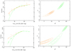 |
Fig. 8. Left columns: luminosity functions for blue galaxies in high (green) and low σ (orange) clusters (top) and for low LX (orange) and high LX (green) clusters (bottom). Right columns: corresponding error ellipses. Again, care should be taken over the interpretation of the fitted parameters given the quality of the fits, though it is clear when simply looking at the data points that at least in the case of splitting by X-ray luminosity, there is a clear difference by the two subsamples. Continous and dashed lines and contours have the same meaning as in Fig. 6. The dashed line and contours for the split by X-ray luminosity show the (improved) fit for the high Lx subsample when only ranging over the same NUV0 values as for the low Lx subsample. In this case, the faint end slopes between the two subsamples are similar and the main difference is in a ∼1 mag shift in M*, it being fainter for the high Lx subsample. |
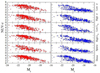 |
Fig. 9. Colour-magnitude diagrams in NUV − r vs. Mr for optically red (red symbols, left panels) and blue (blue symbols, right panels) galaxies in each of the cluster subsamples we consider, as indicated in the legend to the right of each subpanel. Note that the sample is selected in NUV and is therefore not complete in r. |
We plot the NUV − r against Mr colour magnitude distributions for all the subsamples in Fig. 9 to understand the origin of these differences. As expected red sequence galaxies do not appear to show significant differences according to cluster environment, as most of their stellar populations are old and little significant star formation is likely to take place in these systems. Perhaps the only notable variation is that in sparse systems there appear to be a higher proportion of optically red galaxies with relatively blue NUV − r and in comparison to the dense systems a smaller proportion of massive optically red galaxies with NUV – r > 5. Together, this may indicate that some sporadic low level star formation (contributing only to the UV flux) may persist in red galaxies in sparse environments. There appear to be more significant variations for blue galaxies. The most significant is an excess of optically massive blue galaxies (Mr < − 20) with red NUV − r colours in comparison to the number of lower mass blue galaxies with blue NUV − r colours in clusters of low X-ray luminosity, compared to galaxies within clusters in the high X-ray luminosity subsample. Also, in the same subsamples it appears that almost all of the blue galaxies with Mr < − 20 and 3 < NUV – r < 5 (the NUV green valley, Salim 2014) fall in the low Lx subsample. This may indicate either a slower fading of UV emission as star formation is quenched in the low Lx sample or that any sporadic restarting or flickering of star formation is completely suppressed in the high Lx sample, i.e., quenching in the high Lx clusters allows for no restarting (even temporarily) of some star formation, presumably due to highly effective or decisive removal/disruption of the fuelling gas supply.
4. Discussion
We have derived a composite LF for 6471 NUV-selected galaxies in 28 low redshift clusters, with highly complete redshift coverage, and examined how these composite LFs depend on cluster properties and how red sequence and blue cloud galaxies are affected by their environment, especially as regards star formation
We find that the cluster UV LF has M* comparable, or slightly brighter, than the field but has a considerably steeper faint end slope. Our results are in good agreement with measurements in Coma and the Shapley supercluster, but Virgo and the outer regions of Coma have flatter LFs and fainter M*. By splitting our data into several subsamples, we argue that these variations are due to small number statistics when looking at the bright (and sparsely populated) end of single clusters.
The steeper slope in clusters appears to be due to the contribution from NUV-faint but optically bright early-type galaxies, that are common and prominent in clusters but nearly absent in the field (as originally argued by Cortese et al. 2008 and Haines et al. 2011). The LF is steeper as a result of sampling the exponentially rising part of the galaxy mass function and because NUV–optical colours of quiescent galaxies are dominated by hot horizontal branch stars, rather than ongoing star formation, and become bluer for higher luminosities (and masses) – though never as blue as for strong ongoing star formation, as shown in Fig. 5. The slope of the LF therefore may depend on the sampling depths to some extent (as pointed out by Boselli et al. 2016a).
The total LF does not appear to change with velocity dispersion of the clusters but appears to have some dependence on X-ray luminosity and local density. This may favour models where interactions with the X-ray gas (e.g., ram pressure stripping) affect the star formation properties of galaxies as they fall within clusters as both of these environmental parameters correlate with intra cluster medium density.
For this reason we have considered red and blue galaxies separately as it may be expected that the blue population is affected more by environment than the red. Our blue galaxy LF is similar to that determined for other individual clusters, showing that environmental effects are either weak or that star-forming galaxies within clusters are a transitional population, observed during a brief period prior to their quenching. Therefore the apparent universality of the blue galaxy LF may be interpreted as a selection effect as in Cortese et al. (2008).
Unfortunately, the LFs we derive for red galaxies are quite uncertain and noisy. In all cases, a few bright galaxies distort the LF, so that the fit to a single Schechter function is quite poor. Taken at face value, the red LFs are relatively steep, but the dynamic range is small and the values we derive for the fit have large errors.
For blue galaxies we are able to observe that M* becomes fainter in high σ and high LX clusters, compared to low σ and low LX clusters, while the behaviouer of α depends on the range of NUV0 that is fitted to (see Fig. 7). In any event the ratio of UV luminous to faint galaxies is lower in the higher velocity dispersion and Lx cluster subsamples (i.e., the more massive clusters). This suggests that star formation is being suppressed in giant galaxies in these environments. Based on the NUV luminosities and the apparent difference in fitted M* between subsamples, the star formation rates of the most vigorous star forming galaxies appears to decline by a factor of approximately 4–5 between the two groups of clusters with low and high X-ray luminosity. The variation we see between the high and low density subsamples may be consistent with the observation of Boselli et al. (2016a) that the slope of the Virgo cluster’s UV LF flattens from the periphery to the cluster core (i.e., low to high density).
It is not clear whether velocity dispersion or X-ray luminosity is the most important parameter affecting ongoing star formation, but of course high-mass clusters tend to have both higher velocity dispersion and X-ray luminosity, while the few high σ clusters that are underluminous in X-rays may be recent mergers. However, the blue galaxies LFs for low and high X-ray luminosity clusters appear to differ more than the equivalent LFs for high and low velocity dispersion clusters, which may indicate that effects such as (gas-dependent) ram stripping may be more important than (galaxy-dependent) mergers and interactions. Indeed, we may expect that in clusters with high σ these latter effects will be less relevant, although harassment and flybys may be more effective in these cases.
Our data suggest that while bright red sequence galaxies are comparatively unaffected by the cluster environment (as their NUV emission derives from old stellar populations), there should be significant populations of fainter red galaxies showing the effects of recent quenching. Deeper FUV and NUV observations of nearby clusters with existing and upcoming instrumentation would be needed to confirm this hypothesis, such galaxies are potentially missing from our samples due to our NUV flux limit.
Clearly interpretation of the luminosity functions that we have presented is potentially complicated by the range in the quality of the Schechter function fit to the various subsamples obtained by splitting the data set into two equal halves dependent of different cluster parameters. While one pair of subsamples may be well fitted, a different split of the same data may lead to luminosity distributions that are not well fit by Schechter functions. Nevertheless, by focussing where necessary on the ratio of UV bright to faint galaxies in particular pairs of subsamples, we have been able to estrablish clear, robust differences in their luminosity functions.
Acknowledgments
The PanSTARRS1 Surveys (PS1) and the PS1 public science archive have been made possible through contributions by the Institute for Astronomy, the University of Hawaii, the PanSTARRS Project Office, the Max-Planck Society and its participating institutes, the Max Planck Institute for Astronomy, Heidelberg and the Max Planck Institute for Extraterrestrial Physics, Garching, The Johns Hopkins University, Durham University, the University of Edinburgh, the Queen’s University Belfast, the Harvard-Smithsonian Center for Astrophysics, the Las Cumbres Observatory Global Telescope Network Incorporated, the National Central University of Taiwan, the Space Telescope Science Institute, the National Aeronautics and Space Administration under Grant No. NNX08AR22G issued through the Planetary Science Division of the NASA Science Mission Directorate, the National Science Foundation Grant No. AST-1238877, the University of Maryland, Eotvos Lorand University (ELTE), the Los Alamos National Laboratory, and the Gordon and Betty Moore Foundation. This research has made use of the NASA/IPAC Extragalactic Database (NED) which is operated by the Jet Propulsion Laboratory, California Institute of Technology, under contract with the National Aeronautics and Space Administration. This research has made use of the SIMBAD database, operated at CDS, Strasbourg, France. This research has made use of the VizieR catalogue access tool, CDS, Strasbourg, France. The original description of the VizieR service was published in A&AS 143, 23. This research has made use of the X-Rays Clusters Database (BAX) which is operated by the Laboratoire d’Astrophysique de Tarbes-Toulouse (LATT), under contract with the Centre National d’Etudes Spatiales (CNES). We acknowledge the referee for his/her perceptive commentary.
References
- Ali, S., Bremer, M. N., Phillipps, S., & De Propris, R. 2018, MNRAS, 476, 1010 [NASA ADS] [CrossRef] [Google Scholar]
- Andreon, S. 1999, A&A, 351, 65 [NASA ADS] [Google Scholar]
- Beers, T. C., Kage, J. A., Preston, G. W., & Shectman, S. A. 1990, AJ, 100, 849 [NASA ADS] [CrossRef] [Google Scholar]
- Blanton, M. R., Hogg, D. W., Bahcall, N. A., et al. 2003, ApJ, 592, 819 [NASA ADS] [CrossRef] [Google Scholar]
- Böhringer, H., Chon, G., & Collins, C. A. 2014, A&A, 570, A31 [NASA ADS] [CrossRef] [EDP Sciences] [Google Scholar]
- Böhringer, H., Chon, G., Retzlaff, J., et al. 2017, AJ, 153, 220 [NASA ADS] [CrossRef] [Google Scholar]
- Boselli, A., Voyer, E., Boissier, S., et al. 2014, A&A, 570, A69 [NASA ADS] [CrossRef] [EDP Sciences] [Google Scholar]
- Boselli, A., Boissier, S., Voyer, E., et al. 2016a, A&A, 585, A2 [NASA ADS] [CrossRef] [EDP Sciences] [Google Scholar]
- Boselli, A., Roehlly, Y., Fossati, M., et al. 2016b, A&A, 596, A11 [NASA ADS] [CrossRef] [EDP Sciences] [Google Scholar]
- Bremer, M., Phillipps, S., Kelvin, L., et al. 2018, MNRAS, 476, 12 [NASA ADS] [CrossRef] [Google Scholar]
- Carlberg, R. G., Yee, H. K. C., Ellingson, E., et al. 1997, ApJ, 485, L13 [NASA ADS] [CrossRef] [Google Scholar]
- Cava, A., Bettoni, D., Poggianti, B. M., et al. 2009, A&A, 495, 707 [NASA ADS] [CrossRef] [EDP Sciences] [Google Scholar]
- Chambers, K. C., Magnier, E. A., Metcalfe, N., et al. 2016, ArXiv e-prints [arXiv:1612.05560] [Google Scholar]
- Colless, M. 1989, MNRAS, 237, 799 [NASA ADS] [CrossRef] [Google Scholar]
- Cortese, L., Gavazzi, G., Boselli, A., et al. 2003, A&A, 410, L25 [NASA ADS] [CrossRef] [EDP Sciences] [Google Scholar]
- Cortese, L., Boselli, A., Gavazzi, G., et al. 2005, ApJ, 623, L17 [NASA ADS] [CrossRef] [Google Scholar]
- Cortese, L., Gavazzi, G., & Boselli, A. 2008, MNRAS, 390, 1282 [NASA ADS] [CrossRef] [Google Scholar]
- Darvish, B., Martin, C., Gonçalves, T. S., et al. 2018, ApJ, 853, 155 [NASA ADS] [CrossRef] [Google Scholar]
- De Propris, R. 2017, MNRAS, 465, 4035 [NASA ADS] [CrossRef] [Google Scholar]
- De Propris, R., Colless, M., Driver, S. P., et al. 2003, MNRAS, 342, 725 [NASA ADS] [CrossRef] [Google Scholar]
- Flewelling, H. A., Magnier, E. A., Chambers, K. C., et al. 2016, ArXiv e-prints [arXiv:1612.05243] [Google Scholar]
- Gullieuszik, M., Poggianti, B., Fasano, G., et al. 2015, A&A, 581, A41 [NASA ADS] [CrossRef] [EDP Sciences] [Google Scholar]
- Haines, C. P., Busarello, G., Merluzzi, P., et al. 2011, MNRAS, 412, 127 [NASA ADS] [CrossRef] [Google Scholar]
- Hambly, N. C., Irwin, M. J., & MacGillivray, H. T. 2001a, MNRAS, 326, 1295 [Google Scholar]
- Hambly, N. C., MacGillivray, H. T., Read, M. A., et al. 2001b, MNRAS, 326, 1279 [NASA ADS] [CrossRef] [Google Scholar]
- Hammer, D. M., Hornschemeier, A. E., Salim, S., et al. 2012, ApJ, 745, 177 [NASA ADS] [CrossRef] [Google Scholar]
- Henriques, B. M. B., White, S. D. M., Thomas, P. A., et al. 2015, MNRAS, 451, 2663 [NASA ADS] [CrossRef] [Google Scholar]
- Magnier, E. A., Schlafly, E. F., Finkbeiner, D. P., et al. 2016, ArXiv e-prints [arXiv:1612.05242] [Google Scholar]
- Martin, D. C., Fanson, J., Schiminovich, D., et al. 2005, ApJ, 619, L1 [Google Scholar]
- Mitchell, P. D., Lacey, C. G., Lagos, C. D. P., et al. 2018, MNRAS, 474, 492 [NASA ADS] [CrossRef] [Google Scholar]
- Mobasher, B., Colless, M., Carter, D., et al. 2003, ApJ, 587, 605 [NASA ADS] [CrossRef] [Google Scholar]
- Moretti, A., Bettoni, D., Poggianti, B. M., et al. 2015, A&A, 581, A11 [NASA ADS] [CrossRef] [EDP Sciences] [Google Scholar]
- Moretti, A., Gullieuszik, M., Poggianti, B., et al. 2017, A&A, 599, A81 [NASA ADS] [CrossRef] [EDP Sciences] [Google Scholar]
- Morrissey, P., Conrow, T., Barlow, T. A., et al. 2007, ApJS, 173, 682 [NASA ADS] [CrossRef] [Google Scholar]
- Piffaretti, R., Arnaud, M., Pratt, G. W., Pointecouteau, E., & Melin, J.-B. 2011, A&A, 534, A109 [NASA ADS] [CrossRef] [EDP Sciences] [Google Scholar]
- Rodrigues, L. F. S., Vernon, I., & Bower, R. G. 2017, MNRAS, 466, 2418 [NASA ADS] [CrossRef] [Google Scholar]
- Rudnick, G., von der Linden, A., Pelló, R., et al. 2009, ApJ, 700, 1559 [NASA ADS] [CrossRef] [Google Scholar]
- Sadat, R., Blanchard, A., Kneib, J.-P., et al. 2004, A&A, 424, 1097 [NASA ADS] [CrossRef] [EDP Sciences] [Google Scholar]
- Salim, S. 2014, Serb. Astron. J., 189, 1 [Google Scholar]
- Schlafly, E. F., & Finkbeiner, D. P. 2011, ApJ, 737, 103 [NASA ADS] [CrossRef] [Google Scholar]
- Schombert, J. M. 2016, AJ, 152, 214 [NASA ADS] [CrossRef] [Google Scholar]
- Taranu, D. S., Hudson, M. J., Balogh, M. L., et al. 2014, MNRAS, 440, 1934 [NASA ADS] [CrossRef] [EDP Sciences] [PubMed] [Google Scholar]
- Valentinuzzi, T., Poggianti, B. M., Fasano, G., et al. 2011, A&A, 536, A34 [NASA ADS] [CrossRef] [EDP Sciences] [Google Scholar]
- Wyder, T. K., Treyer, M. A., Milliard, B., et al. 2005, ApJ, 619, L15 [Google Scholar]
Appendix A: Additional figures
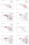 |
Fig. A.1. continued. |
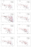 |
Fig. A.1. continued. |
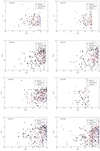 |
Fig. A.2. continued. |
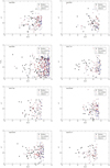 |
Fig. A.2. continued. |
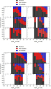 |
Fig. A.3. Completeness fractions for all clusters (see caption of Fig. 3). The numbers refer to the order in Table 1. |
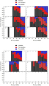 |
Fig. A.3. continued. |
All Tables
Schechter function parameters when fitted to full available NUV0 range for each subsample.
Schechter function parameters for blue galaxies when fitted over full available range of NUV0 for each subsample.
All Figures
|
Fig. 1. Colour-magnitude diagrams in g − r (or BJ − RF) vs. r for NUV-selected galaxies in our clusters. Symbols as identified in the figure legends. Here we show a representative sample of objects. All remaining clusters are shown in Fig. A.1 |
| In the text | |
|
Fig. 2. Same as Fig. 1 but for g − r vs. NUV, with the same symbols (as indicated in the figure legend). This shows that NUV bright cluster members tend to be optically blue while the massive red sequence galaxies are generally faint in NUV. All remaining clusters are shown in Fig. A.2. |
| In the text | |
|
Fig. 3. Completeness fractions for each cluster vs. NUV0 magnitude (in the z = 0.05 bins described in the text). The numbers in the top left corner of each panel identify the cluster, in the order shown in Table 1 (here 1: Abell S1171; 2: Abell 2734; 3: EDCC 442; 4: Abell 85; 5: Abell 119; 6: Abell 168). The symbols used in the plot are identified in the figure legend. All remaining clusters are shown in Fig. A.3. |
| In the text | |
|
Fig. 4. Luminosity function and best fit for all clusters in the sample (top). Error ellipses for 1, 2 and 3σ are shown (bottom). In this and subsequent figures M* refers to the observed characteristic magnitude of the LF measured at z = 0.05. |
| In the text | |
|
Fig. 5. Luminosity function and best fit for red and blue galaxies (identified by colour) for all clusters in the sample (left). Error ellipses for 1, 2 and 3σ are shown in the right-hand panel, for red and blue galaxies. |
| In the text | |
|
Fig. 6. For all galaxies in all clusters we plot the absolute magnitudes in r vs. the absolute magnitudes in NUV on the top panel. Red symbols are for red sequence galaxies and blue symbols for blue cloud galaxies. On the bottom panel we show the NUV-r colours as a function of absolute NUV magnitude. |
| In the text | |
|
Fig. 7. Luminosity functions and best fits left column) and associated error ellipse (right column) for low (orange) and high (green) σ clusters (top row), low (orange) and high (green) LX clusters (middle row) and sparse (orange) and dense (green) clusters (bottom row). The circle in each figure indicates the M* and α values for the total LF. Clearly, for the subsamples split by X-ray luminosity and surface density, the luminosity distributions as sampled here are not well fitted by Schechter functions, the location and size of the error ellipses in these cases should be used with caution. Any interpretation should take note of the actual numbers rather than the fits to the data. The continuous lines and contours are the fits to the entire range of NUV0 values available for a given subsample. The dashed lines and contours are for Schechter fits restricted in range in NUV0 where both subsamples have data. Clearly, in the case of splitting by Lx, even this does not result in a good fit for the high Lx subsample, though obviously the data imply a lower ratio of high to low LUV galaxies in the high Lx subsample relative to that of the low Lx subsample. For the split by surface density, restricting the fitting range has no real effect. |
| In the text | |
|
Fig. 8. Left columns: luminosity functions for blue galaxies in high (green) and low σ (orange) clusters (top) and for low LX (orange) and high LX (green) clusters (bottom). Right columns: corresponding error ellipses. Again, care should be taken over the interpretation of the fitted parameters given the quality of the fits, though it is clear when simply looking at the data points that at least in the case of splitting by X-ray luminosity, there is a clear difference by the two subsamples. Continous and dashed lines and contours have the same meaning as in Fig. 6. The dashed line and contours for the split by X-ray luminosity show the (improved) fit for the high Lx subsample when only ranging over the same NUV0 values as for the low Lx subsample. In this case, the faint end slopes between the two subsamples are similar and the main difference is in a ∼1 mag shift in M*, it being fainter for the high Lx subsample. |
| In the text | |
|
Fig. 9. Colour-magnitude diagrams in NUV − r vs. Mr for optically red (red symbols, left panels) and blue (blue symbols, right panels) galaxies in each of the cluster subsamples we consider, as indicated in the legend to the right of each subpanel. Note that the sample is selected in NUV and is therefore not complete in r. |
| In the text | |
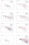 |
Fig. A.1. Colour-magnitude relations for all clusters (see caption of Fig. 1). |
| In the text | |
|
Fig. A.1. continued. |
| In the text | |
|
Fig. A.1. continued. |
| In the text | |
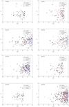 |
Fig. A.2. NUV colour magnitude diagrams (see caption of Fig. 2). |
| In the text | |
|
Fig. A.2. continued. |
| In the text | |
|
Fig. A.2. continued. |
| In the text | |
|
Fig. A.3. Completeness fractions for all clusters (see caption of Fig. 3). The numbers refer to the order in Table 1. |
| In the text | |
|
Fig. A.3. continued. |
| In the text | |
Current usage metrics show cumulative count of Article Views (full-text article views including HTML views, PDF and ePub downloads, according to the available data) and Abstracts Views on Vision4Press platform.
Data correspond to usage on the plateform after 2015. The current usage metrics is available 48-96 hours after online publication and is updated daily on week days.
Initial download of the metrics may take a while.