| Issue |
A&A
Volume 618, October 2018
|
|
|---|---|---|
| Article Number | A174 | |
| Number of page(s) | 9 | |
| Section | Stellar structure and evolution | |
| DOI | https://doi.org/10.1051/0004-6361/201833574 | |
| Published online | 26 October 2018 | |
Non-synchronous rotations in massive binary systems
HD 93343 revisited⋆
1
Instituto de Astrofísica de La Plata (CONICET-UNLP), Paseo del Bosque s/n, 1900 La Plata, Argentina
e-mail: This email address is being protected from spambots. You need JavaScript enabled to view it.
2
Facultad de Ciencias Astronómicas y Geofísicas, Universidad Nacional de La Plata, Paseo del Bosque s/n, 1900 La Plata, Argentina
3
Las Campanas Observatory, Carnegie Observatories, Casilla 601, La Serena, Chile
4
Instituto de Astrofísica de Canarias, 38200, La Laguna, Tenerife, Spain
5
Departamento de Astrofísica, Universidad de La Laguna, 38205, La Laguna Tenerife, Spain
6
Departamento de Física y Astronomía, Universidad de La Serena, Av. Cisternas 1200 Norte, La Serena, Chile
Received:
5
June
2018
Accepted:
22
July
2018
Abstract
Context. Most massive stars are in binary or multiple systems. Several massive stars have been detected as double-lined spectroscopic binaries and among these, the OWN Survey has detected a non-negligible number whose components show very different spectral line broadening (i.e., projected rotational velocities). This fact raises a discussion about the contributing processes, such as angular-momentum transfer and tidal forces.
Aims. We seek to constrain the physical and evolutionary status of one of such systems, the O+O binary HD 93343.
Methods. We analyzed a series of high-resolution multiepoch optical spectra to determine the orbital parameters, projected rotational velocities, and evolutionary status of the system.
Results. HD 93343 is a binary system comprised of two O7.5 Vz stars that each have minimum masses of approximately 22 M⊙ in a wide and eccentric orbit (e = 0.398±0.004; P = 50.432±0.001 d). Both stars have very similar stellar parameters, and hence ages. As expected from the qualitative appearance of the combined spectrum of the system, however, these stars have very different projected rotational velocities (~65 and ~325 km s−1, respectively).
Conclusions. The orbits and stellar parameters obtained for both components seem to indicate that their youth and relative separation is enough to discard the effects of mass transfer and tidal friction. Thus, non-synchronization should be intrinsic to their formation.
Key words: binaries: spectroscopic / stars: early-type / stars: rotation / stars: individual: HD 93343
This work is based on observations collected at Complejo Astronómico El Leoncito, Las Campanas Observatory, and La Silla Observatory.
© ESO 2018
1. Introduction
Massive stars play a key role in the evolution of Universe. Their high luminosities and strong stellar winds sweep away interstellar medium and drive the chemical evolution of galaxies. Usually, these objects are located in star-forming regions, thereby heating and enriching neighboring gas clouds where new generations of stars form. In spite of their importance, there are still many missing pieces in our knowledge about the formation and evolution of these cosmic engines. This is partly because their numbers are low and they are highly complex objects.
In recent years, it has become clear that a high percentage of massive stars are part of binary or multiple systems (Mason et al. 1998; Sana & Evans 2011; Duchêne & Kraus 2013; Sana 2017). The presence of a nearby companion changes the evolutionary path of the individual components in the system (Sana et al. 2012) by means of non-negligible tidal forces, mass exchange, and even transfer of angular momentum. During the mass transfer process, the primary may also transfer angular momentum to the secondary, which is thereby spun up (Wellstein et al. 2001; Petrovic et al. 2005; de Mink et al. 2013). The efficiency of this process is not well understood and constitutes one of the largest uncertainties in binary evolution.
The initial distribution of rotational velocities of massive O-type stars, which is not well known yet (Rosen et al. 2012), could be modified by such a scenario. Ramírez-Agudelo et al. (2013, 2015) have compared the spin distribution of O-type binary components and presumably single stars in the 30 Doradus region of the LMC. They found these objects to be similar as a whole, but some important differences can be clearly distinguished.
The OWN Survey (Barbá et al. 2010, 2014, 2017) is a spectroscopic monitoring program that aims at observing, with high resolution and signal-to-noise ratio (S/N), a sample of Southern O- and WN-type stars. This survey was started in 2005 and, so far, it has collected about 6700 spectra for ~200 stars, comprising a time sampling per target of at least three epochs. This huge database has allowed the identification of more than 100 radial velocity (RV) variable stars, the determination of orbits for about 50 new binary systems (most of them still unpublished), and the discovery of some stars showing line-profile variability. Among the new findings, we identified some double line spectroscopic binaries presenting two sets of line profiles affected by a different amount of rotational broadening, respectively.
There are other known examples of systems showing different line broadenings. We note the following examples: (i) The components in HD 37366, which have projected rotational velocities of 30 and 100 km s−1 and are in an eccentric orbit (e = 0.33) of 31.9 d (Boyajian et al. 2007); (ii) Plaskett’s star (HD 47129), whose components have projected rotations of ~75 and ~300 km s−1 (P = 14.396 d) as measured by Linder et al. (2008); (iii) the components Aa and Ab in the hierarchical multiple system ˙ Ori AB, which have velocities of 135 and 35 km s−1 (P = 143.198 d; Simón-Díaz et al. 2011a, 2015); and (iv) those in HD 101131, which have velocities of 102 and 164 km s−1 in a orbital period of 9.65 d (Gies et al. 2002). Double-lined spectra found in the OWN Survey would be due to a binary system, but this hypothesis has to be tested with RV analysis. If confirmed, the different line broadening could be related to asynchronous rotation or different inclinations of the rotation axis of each component; this, in turn, could be related to the origin of the binary or its evolution (Hut 1981).
This work is the first in a series of papers in which we seek to characterize stars showing such composite spectra. We explore the possibility of dealing with binary systems whose components are asynchronous rotators, starting with HD 93343.
HD 93343 (CPD –59 2633; RA2000 = 10:45:12.2; Dec2000 = −59:45:00.4; V = 9.6 mag) is an O-type double-lined spectroscopic binary star that is member of the young cluster Trumpler 16. Walborn (1982) determined a spectral type of O7 V(n) and noted the presence of spectral features belonging to a secondary component by first time. Although its RVs have been widely studied by many researchers for decades (e.g., Levato et al. 1991; Solivella & Niemela 1998), the SB2 nature of HD 93343 was only confirmed by Rauw et al. (2009). These authors inferred spectral types O7–8.5 and O8 for the primary and secondary components, respectively, but were not able to establish an orbital solution. Their data also revealed that the secondary component has broadened lines. Sota et al. (2014) did not detect double lines in their low-resolution data but classified the composite spectrum as O8 Vz. Maíz Apellániz et al. (2016) reclassified the star, removing the qualifier “z”, but retaining the O8 V spectral type. Putkuri et al. (2016) published a preliminary orbital solution for both components and obtained a mass ratio of 0.87 ± 0.03.
We present the complete analysis of a dataset comprising high-resolution spectra of HD 93343 (see Sect. 2) spanning more than ten years. This paper then presents the individual spectra obtained via spectral disentangling and RV measurements in Sect. 3. In Sects. 4 and 5 we present the determination of the orbital solution and spectroscopic analysis, including spectral classification and determination of the stellar parameters of each component. Finally, we perform an analysis of the evolutionary status of the stars in Sect. 6 and discuss the results and their conclusions in Sect. 7 and 8.
2. Observations
Our observational dataset consists of 40 high-resolution spectra acquired between 1994 and 2017. We employed the 2.15 m J. Sahade telescope at Complejo Astronómico El Leoncito (CASLEO)1, Argentina; the 2.5 m Irénée du Pont telescope at Las Campanas Observatory (LCO), Chile; and the MPG/ESO 2.2 m telescope at La Silla Observatory, Chile. For each of these, we used their échelle spectrographs. First spectra, at CASLEO, were observed in the context of an international campaign called X-Mega (Corcoran 1999). See Table 1 for details of the instrumental configuration used in this work, where in successive columns we give the name of the spectrograph, observatory, time span of each dataset, spectral coverage, resolving power (R), reciprocal dispersion, and number of obtained spectra (n).
Technical details of the instrumental configurations.
At CASLEO and LCO, comparison lamp spectra of Th-Ar were observed immediately after or before each target integration at the same telescope position. All the spectra were extracted and normalized using the standard IRAF2 routines. The FEROS data were reduced using the standard reduction pipeline provided by ESO.
3. Spectral disentangling and radial velocity measurements
To determine the orbital solution of HD 93343, we measured the RVs of both components in the system. For this purpose, we firstly proceeded to disentangle both spectra. We employed a procedure for separating composite spectra based on the code published by González & Levato (2006). It basically consists in combining the composite spectra shifted to the RV of one of the components to dilute the spectral features of the other (e.g., secondary). The spectrum combined in this way contains the features of the primary and those of the secondary diluted (as they are at different wavelengths). Then, this template (almost pure primary component) is subtracted from the original composite spectra (shifted to the same RV) to obtain the spectrum of the other component. These are then combined and shifted to the secondary RV. An initial estimation of the RVs of both components is needed to start the method. Once the initial templates are generated, the method determines the RVs by means of cross-correlation between each template and subtraction of the other template from the composite spectra. It is assumed that these new RVs are more accurate than the initial RVs, and new templates are generated using the new RVs to shift the spectra. This time, the template of the primary is generated subtracting the template of the secondary. After several iterations, the templates tend to represent the pure spectrum of each component
Because of the peculiarities of this system, we decided to consider some variations to the method. Regarding the initial RVs, as the secondary component is very broad and it is very difficult to identify the barycenter of the line, we had to be very careful in this task. We determined the central wavelengths of the spectral lines using the ngauss task of IRAF. The cross-correlation was applied in four different wavelength domains, i.e., 4461–4478 Å, 4536–4549 Å, 4675–4695 Å, and 5863–5887 Å, which include the He Iλλ4471, 5876 and He IIλλ4542, 4686 absorption lines. The RVs of the four lines of the primary component gave similar results (maximum differences ~10 km s−1). These RVs were then averaged to represent the RV of the primary component. For the secondary, the differences among RVs were significantly higher and reached values as high as 60 km s−1 in a few cases. As a consequence, to represent the secondary motion we used the He Iλ5876 line, which certainly appears to be the least affected by pair blending.
The template of the secondary obtained via this raw procedure gave very noisy and almost useless results. We constructed an initial template of the secondary to improve it. We subtracted a synthetic template of the primary component3 to the best composite spectrum obtained during quadratures. In this way, we obtained a template of the secondary component that was used in the first iteration of the disentangling method.
To test the confidence of the method, we constructed composite spectra adding both templates, shifted by the obtained RVs and compared these with the observed spectra. We noted that the secondary spectrum did not fit well. Actually, fitting the broadened features is an issue that we try to illustrate in Fig. 1. There, we plot synthetic spectra, shifted to three different velocities, over an observed spectrum. It can be noted that the differences are subtle, thus errors in RVs could be larger than estimated. Then, we refined the secondary RVs adopting those that minimize the differences, i.e., we always checked the RVs obtained by comparing the original composite spectrum with that constructed from the sum of templates (an example of this is shown in Fig. 2). The final RVs used in the orbital solution are showed in Table 2.
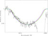 |
Fig. 1. Comparison of observed composite spectrum (in black) with three synthetic templates shifted with different RVs around He Iλ5875. The blue line is shifted by 130 km s−1, red by 140, and green by 150 km s−1. The green curve best fits the spectrum, but the others are not so bad. |
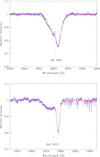 |
Fig. 2. Comparison between observed composite spectra in phase of maximum separation (blue) and the sum of templates shifted with the corresponding RVs of Table 2 (red). Top: around Hβ; bottom: around He Iλ5875. |
4. Orbital solution
We searched for periodicities in our data by means of the NASA Exoplanet Archive Periodogram Service. We employed the Lomb–Scargle (Scargle 1982) method, obtaining a most probable period (P) of 50.45 ± 0.15 d. In Fig. 3 we show the strength (named as power) of the candidate periods.
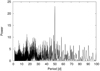 |
Fig. 3. Periodogram of the primary RVs obtained with NASA Exoplanet Archive Periodogram Service. |
With this P as initial value, we determined the orbital solution using the gbart code4, letting all the parameters free. The RVs of CASLEO were weighted by half owing to its lower resolution respect to the LCO and FEROS values. The orbital parameters obtained are given in Table 3 and the RV curves are depicted in Fig. 4. It is important to highlight that the RV amplitude of the secondary component is lower than previously reported by Putkuri et al. (2016), which results in lower minimum masses.
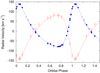 |
Fig. 4. Radial velocity curves of primary (blue) and secondary (red) components of the binary system HD 93343, calculated with the parameters of the orbital solution shown in Table 3. Primary RV errors are smaller than sizes of the symbols. Primary RVs were weighted according the resolution of their spectra, LCO and La Silla data with 1 (filled circles), and CASLEO with 0.5 (open circles). For the secondary all data were weighted with 0.5 (open circles). |
5. Spectroscopic analysis
5.1. Spectral classification
We used the templates resulting from the disentangling method to provide a spectral classification of both components of the binary system. To this aim, we degraded the templates to a resolving power (R) of 2500 and compared these with the set of spectra of O-type standards proposed by Sota et al. (2011) and Maíz Apellániz et al. (2016). In addition, we followed the guidelines for spectral classification of this type of objects indicated in those works.
One of the major criteria for spectral type is the ratio He IIλ4542/He Iλ4471. In both spectra, this ratio resulted in less than unity, thus indicating spectral types later than O7. The ratios He IIλ4542/He Iλ4388 > 1 and He IIλ4200/He Iλ4144 ≫ 1 are in agreement with an O7.5–8 subtype. On the other hand, the ratio He IIλ4686/He Iλ4713 ≫ 1 led to a luminosity class V. The unusually strong absorption in the He IIλ4686 line observed in both templates indicates the addition of the “z” qualifier. The agreement of the template with the O7.5 Vz standard from Maíz Apellániz et al. (2016) is evident for the primary (see Fig. 5) and, because of the high rotational broadening, less clear for the secondary. However the Vz classification for both components is confirmed through the quantitative criterion proposed by Arias et al. (2016), which states that the ratio of the equivalent width of the He IIλ4686 line to the maximum between the equivalent widths of the He Iλ4471 and He IIλ4542 must be greater or equal than 1.1.
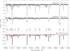 |
Fig. 5. High-resolution disentangled spectra of both components of the binary system HD 93343 (first two solid black lines). Features that are relevant for spectral classification are indicated. Some artifacts appear on the spectrum of the secondary component, mostly in the wings of hydrogen lines that originate in the disentangling process. In the lower box we present the primary component degraded in resolution and overplotted with the O7.5 Vz standard star from Maíz Apellániz et al. (2016, red dashed line). |
Both stars present overall similar spectra as can be seen in Fig. 5, but it can be noticed that C IIIλ4070 presents stronger in the secondary component than in the primary. This could indicate a surface chemical enrichment due to fast rotation, since this favors the transport of heavier elements synthesized in the nucleus toward the outer stellar layers (Meynet & Maeder 2000).
5.2. Quantitative spectroscopic analysis
We employed the iacob-broad tool (Simón-Díaz & Herrero 2014) to obtain estimates for the projected rotational velocity (v sin i) and the macroturbulence broadening (vmac) of each component of the binary system. To this aim, we used the O III 5592 line present in each of the corresponding disentangled spectra (this time not degraded in resolution). As expected from the qualitative appearance of the original composite spectra (see Fig. 2), the derived values of v sin i are very different for the narrow and broad components (~65 and ~325 km s−1, respectively; see also Table 4).
Subsequently, we proceeded with the determination of other spectroscopic parameters such as the effective temperature (Teff) and stellar gravity (log g). To this aim, we first tried to perform a quantitative spectroscopic analysis of the individual disentangled spectra with IACOB-GBAT 5 (Simón-Díaz et al. 2011b). However, we found that the solution provided by IACOB-GBAT was not completely satisfactory, especially in the case of the secondary star, because of the presence of some spurious artifacts affecting the wings of the hydrogen lines (see Fig. 5) introduced during the disentangling process. We hence decided to follow a different approach; namely, the stellar parameters of the two components were obtained directly and simultaneously from the analysis of one of the original spectra. In particular, we considered one of the FEROS spectra with largest separation between lines.
The combined synthetic spectra to be fitted to the observed spectrum were constructed using spectra from the grid of FAST-WIND models with solar metallicity included in IACOB-GBAT. The spectrum of each component was convolved to the corresponding v sin i and vmac, shifted in RV, and scaled by a certain factor di, where Σ di=1. Then, the two synthetic spectra were added together, and the combined spectrum overplotted to the observed spectrum.
During the analysis process, we fixed the associated helium abundances (YHe), microturbulent velocities (ξt), and the two wind parameters considered in the grid of FASTWIND models (β and log Q; see Simón-Díaz et al. 2011b) to characteristic values commonly obtained for Galactic mid O-type dwarfs (basically YHe = 0.10, ξt = 10 km s−1, β = 0.8, log Q = −13.5). Also, given that the orbital solution indicates that the mass ratio of the stars is close to unity, we assumed that both components of the binary system contribute 50% to the global spectrum (i.e., di = 0.5). As a result, only the effective temperatures and gravities remained as free parameters to be determined in the analysis.
The best-fit solution was obtained by visual comparison of the original and combined synthetic spectra around the H and He I-II lines, which are commonly assumed as a diagnosis for the determination of stellar parameters of O stars (e.g., Herrero et al. 1992, 2002; Repolust et al. 2004). The final fit is shown in Fig. 6, where the relative contribution of each component to the global spectrum is also presented. This figure serves to illustrate the quality of the best-fit solution as well as the difficulty in determining precisely the gravity of the two components from the wings of the hydrogen Balmer lines. We note that given the complexity of the analysis and the similarity of both stars, except for the case of the associated projected rotational velocities, we basically obtained the same Teff and log g for the primary and secondary components of the system. The resulting values are summarized in Table 4.
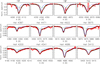 |
Fig. 6. Analysis by FASTWIND of one of the FEROS combined spectra of HD 93343 with largest separation between the lines of both components. Solid red and black lines correspond to the observed spectrum and best combined synthetic spectrum, respectively. The individual best-fit synthetic spectra for each component are overplotted with green and blue dashed lines, respectively. |
To calculate the corresponding radii, luminosities, and spectroscopic masses, the absolute magnitudes of each component are required. On the one hand, we could assume the value provided in the calibration by Martins et al. (2005) for an O7.5 V star (MV = −4.5). On the other hand, the individual absolute magnitudes can be estimated if the distance, apparent magnitude (mV diluted), and amount of extinction (AV) are known. We gleaned these parameters in the available literature and adopted a distance of 2.7 kpc (Gaia Collaboration 2016, 2018). We determined mV and color excess from observational values cited in the Simbad Astronomical Database (Wenger et al. 2000) and intrinsic colors from Wegner (1994). To obtain the absorption AV, we assumed RV = 4.4 ± 0.2 from Hur et al. (2012). Thus, we obtained E(B − V) = 0.53 and AV = 2.33. Using this information and assuming that both stars equally contribute to the total stellar flux, we ended up with an individual absolute magnitude for each component of MV = −4.19. As both approaches result in rather different values of MV, and for comparative purposes, we keep in Table 4 the two associated sets of derived R, L and Msp. Again, we note that the quoted values are representative of both components since we are basically considering the same Teff, log g, and MV.
6. Evolutionary status
We used the Bayesian automatic tool BONNSAI (Schneider et al. 2014)6 to characterize the evolutionary status of the components in the HD 93343 system. The BONNSAI project is a statistical method, which matches the entire available observables (more specifically Teff, log g, log L, and v sin i) simultaneously to stellar models from Brott et al. (2011) while taking observed uncertainties and prior knowledge.
We run BONNSAI using the Teff, log g, and v sin i resulting from the quantitative spectroscopic analysis (see Sect. 5.2), and the two estimates of log L quoted in Table 4. The results are presented in Table 5 and depicted in a Hertzprung-Russell (HR) diagram in Fig. 7. In this figure, we also plot a set of evolutionary tracks and isochrones calculated by Brott et al. (2011) with initial rotational velocities in the range 53–61 km s−1, to represent the primary component, and 320–330 km s−1 (orange) to depict the secondary. As can be seen, both stars are located near the zero age main sequence (ZAMS) between the isochrones of ~3.0 and 3.6 Myr.
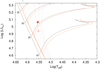 |
Fig. 7. Evolutionary tracks in the HR diagram for stellar masses in the range 20–35 M⊙ taken from Brott et al. (2011). The vertical lines correspond to the isochrones of 1, 2, 3, 3.6, and 4 Myr (dotted lines) and the ZAMS (solid line). Horizontal lines depict the evolutionary tracks: black solid lines identify values of rotational velocities in the range 53– 61 km s−1 (that is, for the primary). Orange, the same for the secondary (rotation in the range 320–330 km s−1). The points represent the location of the HD 93343 binary components (black for the primary and red for the secondary): filled and empty dots for MV from Martins et al. (2005) and for MV estimated from distance modulus calculated in Sect. 5.2, respectively |
We made a series of analyses on the disentangled spectra. Firstly, we confirmed the very different broadening presented by both components, which we visually noted and were also indicated by Rauw et al. (2009). We calculated that the projected rotational velocity of the secondary is about five times that of the primary star. Hence, its spectral features are more diluted in the composite spectrum. However, the spectral type of this star is similar to that of the primary, even the “z” qualifier is appropriate for both stars.
We obtained a different orbital solution than the preliminary published by Putkuri et al. (2016). This time, we revised the secondary RVs very carefully and employed new ways to measure the RVs, i.e., adjusting these values by comparison of the composite original spectrum with that created from the sum of both templates, shifted to the determined RV (see Sect. 3). We found a smaller orbit for the broad component and therefore lower minimum masses than before. In this work, the determined minimum masses are M sin3i ≈ 22 M⊙ for both components, which are nearly those expected for their spectral types. Thus, the orbital inclination should be close to 90°. We performed some raw trials with the PHysics Of Eclipsing BinariEs ( PHOEBE 0.31a version) code (Prša & Zwitter 2005) to our RV data and the photometry published by Rauw et al. (2009) generously provided by E. Fernández Lajús. As no evident eclipses are detected in the light curve, we estimated a maximum orbital inclination of 84°, which would produce sharp eclipses of about 0.01 mag in the threshold of detectability of those data. More accurate photometric observations are critical to determine a reliable inclination, and thus absolute masses of two O7.5 Vz-type stars.
We performed the analysis of the physical properties and evolutionary status employing the IACOB-GBAT and BONNSAI tools. The range of initial evolutionary masses obtained for both stars, i.e., 23–26 M⊙, is well within the errors of the dynamical spectroscopic mass (M sin3i ≈ 22 M⊙). On the other hand, the spectroscopic masses (~16–21 M⊙) resulted in values considerably lower than those. This is a long-standing problem known as mass discrepancy (Herrero et al. 1992). It is tailored discussed in Markova et al. (2018), where the discrepancy seems to be more evident in the range of masses around 20 M⊙ (see their Fig. 11).
7. Discussion
It is important to note the role of rotational broadening on the Vz phenomenon. Sabín-Sanjulián et al. (2014) found that higher values of v sin i generally favor the Vz characteristic at relatively low temperatures (Teff < 38 000 K), they also found that at an intermediate range of temperatures, between 35 000 K and 40 000 K, a star with a modest wind strength also appears as Vz. Nevertheless, the position of both components of HD 93343 in the HR diagram seems to point out the youth of the system. We crudely estimated the timescales for synchronization (tsync) and circularization (tcirc) for the system by means of the expressions given by Zahn (1977). For this, we used the grid of stellar models by Claret (2004), considering stellar masses of ~20 M⊙ and extrapolating the term of moment of inertia (I/MR 2) from the data provided by Zahn (1975) in tabular form, as a function of stellar mass. For our system we find tsync ~ 6 × 10⁸ years and tcirc ~ 8 × 10¹¹ years. The strong dependence of tsync and tcirc on the ratio a/R produces, for this wide binary, timescales for synchronization and circularization that are much larger than the estimated age of the system.
Exploring the origin of the asynchronous rotation of both components, we analyzed the mass transfer scenario. In order to determine whether or not a star fills its critical Roche lobe, that is, if the stellar radius attains the radius of the sphere with a volume equal to that of the Roche lobe (Rst = RL), we calculated the Roche lobe radii of the system during the periastron passage. This can be approximated by Eq. (45) of Sepinsky et al. (2007), i.e.,  . We found
  and
and  for the primary and secondary, respectively. These results imply that the stellar radii are well inside (~40%) the respective Roche lobes. Hence, mass and angular momentum exchange should not have started yet and both stars are evolving independently, i.e., following single-star evolution so far.
The idea that in close binaries the rapid rotation is reached when the mass transfer is accompanied by angular momentum exchange (Packet 1981) is not applicable here. The scenario of HD 93343 is very different: it is a young, eccentric, and wide binary that has components whose radii occupy little volume of their respective Roche lobes and whose projected rotational velocities are considerably different. Thus, the fact that this system is asynchronous should be related to its formation ambient.
8. Conclusions
We have observed the spectroscopic massive binary HD 93343 obtaining a set of high quality spectra, which allowed us to apply the disentangling technique of González & Levato (2006) to calculate the individual spectra, and classify both of these as O7.5 Vz.
We measured the RVs in each obtained spectrum using the individual disentangled spectra (see Sect. 3) and determined a new SB2 orbital solution. The system resulted in a wide (P = 50.432 ± 0.001 d) and eccentric (e = 0.398 ± 0.004) orbit.
The stellar physical parameters were obtained directly from the quantitative spectroscopic analysis of one of the original FEROS spectra, where the lines of the stars are best separated (see Sect. 6 for details and Table 4 for results). The major difference between components is the projected rotational velocities of 63 and 330 km s−1 for the narrow and broad component, respectively.
The dynamical minimum masses obtained agree with the spectroscopic masses (computed via the IACOB-GBAT tool), and the evolutionary masses (estimated by means of BONNSAI) and are also in agreement with the masses expected from the observational Teff scales by Martins et al. (2005).
The evolutionary status of the components in the system, i.e., the evolutionary masses and ages, was characterized by means the BONNSAI tool. An age of 3.4–3.8 Myr was derived, depending on the adopted MV. Following Martins & Palacios (2013), a 20–30 M⊙ star reaches the terminal age main sequence (TAMS) in about 8–9 Myr and spends 80% of this time in the dwarf phase (Martins & Palacios 2017), hence the system is closer to the ZAMS than the TAMS. Thus, their comparative youth and the obtained radius (well inside their respective Roche lobes), indicate that no star has experienced Roche lobe overflow and an exchange of matter or angular momentum has not occurred yet.
Combining findings from this study, i.e., the very different projected rotational velocities, their youth, and the wide orbit, we can conclude that the spins of the two components are not synchronized. The current rotational configuration should be intrinsic to the birth of the system. We will continue our study with the other systems in the sample, looking for possible relations between asynchronism, eccentricity, orbital period, and age.
Complejo Astronómico El Leoncito is operated under agreement between the Consejo Nacional de Investigaciones Científicas y Técnicas de la República Argentina and the National Universities of La Plata, Córdoba and San Juan.
IRAF is distributed by the National Optical Astronomy Observatories, which are operated by the Association of Universities for Research in Astronomy, Inc., under cooperative agreement with the National Science Foundation.
We used as synthetic template the best-fitting FASTWIND model resulting from the quantitative spectroscopic analysis (see Sect. 5).
Based on the algorithm of Bertiau & Grobben (1969) and implemented by F. Bareilles (available at http://www.iar.unlp.edu.ar/~fede/pub/gbart).
The IACOB grid-based algorithm tool ( IACOB-GBAT) is a user-friendly IDL package based on standard techniques for the quantitative spectroscopic analysis of O stars, which has been automated by applying a χ 2 algorithm to a large grid of synthetic spectra computed with the FAST-WIND stellar atmosphere code (Santolaya-Rey et al. 1997; Puls et al. 2005; Rivero González et al. 2011). Recent applications of this tool can be found in Sabín-Sanjulián et al. (2014, 2017) and Holgado et al. (2018).
The BONNSAI web-service is available at www.astro.uni-bonn.de/stars/bonnsai.
Acknowledgments
We thank the referee for her/his valuable comments and suggestions. CP, RG, NM, GF, and GS are Visiting Astronomers, Complejo Astronómico El Leoncito operated under agreement between the Consejo Nacional de Investigaciones Científicas y Técnicas de la República Argentina and the National Universities of La Plata, Córdoba and San Juan. We thank the directors and staff of CASLEO, LCO, and La Silla/ESO for support and hospitality during our observing runs. This work has made use of data from the European Space Agency (ESA) mission Gaia (https://www.cosmos.esa.int/gaia), processed by the Gaia Data Processing and Analysis Consortium (DPAC, https://www.cosmos.esa.int/web/gaia/dpac/consortium). Funding for the DPAC has been provided by national institutions, in particular the institutions participating in the Gaia Multilateral Agreement. S.S.-D. acknowledges financial support from the Spanish Ministry of Economy and Competitiveness (MINECO) through grants AYA2015-68012-C2-1 and Severo Ochoa SEV-2015-0548, and grant ProID2017010115 from the Gobierno de Canarias.
References
- Arias, J. I., Walborn, N. R., Simón Díaz, S., et al. 2016, AJ, 152, 31 [NASA ADS] [CrossRef] [Google Scholar]
- Barbá, R. H., Gamen, R., Arias, J. I., et al. 2010, Rev. Mex. Astron. Astrofis. Conf. Ser., 38, 30 [NASA ADS] [Google Scholar]
- Barbá, R., Gamen, R., Arias, J. I., et al. 2014, Rev. Mex. Astron. Astrofis. Conf. Ser., 148, 44 [Google Scholar]
- Barbá, R. H., Gamen, R., Arias, J. I., & Morrell, N. I. 2017, in The Lives and Death-Throes of Massive Stars, eds. J. J. Eldridge, J. C. Bray, L. A. S. McClelland, & L. Xiao, IAU Symp., 329, 89 [NASA ADS] [Google Scholar]
- Bertiau, F. C., & Grobben, J. 1969, Ric. Astron., 8, 1 [Google Scholar]
- Boyajian, T. S., Gies, D. R., Dunn, J. P., et al. 2007, ApJ, 664, 1121 [NASA ADS] [CrossRef] [Google Scholar]
- Brott, I., de Mink, S. E., Cantiello, M., et al. 2011, A&A, 530, A115 [NASA ADS] [CrossRef] [EDP Sciences] [Google Scholar]
- Claret, A. 2004, A&A, 424, 919 [NASA ADS] [CrossRef] [EDP Sciences] [Google Scholar]
- Corcoran, M. F. 1999, in Rev. Mex. Astron. Astrofis. Conf. Ser., eds. N. I. Morrell, V. S. Niemela, & R. H. Barbá, 27, 8, 131 [NASA ADS] [Google Scholar]
- de Mink, S. E., Langer, N., Izzard, R. G., Sana, H., & de Koter, A. 2013, ApJ, 764, 166 [NASA ADS] [CrossRef] [Google Scholar]
- Duchêne, G., & Kraus, A. 2013, ARA&A, 51, 269 [Google Scholar]
- Gaia Collaboration (Prusti, T., et al.) 2016, A&A, 595, A1 [NASA ADS] [CrossRef] [EDP Sciences] [Google Scholar]
- Gaia Collaboration (Brown, A. G. A., et al.) 2018, A&A, 616, A1 [NASA ADS] [CrossRef] [EDP Sciences] [Google Scholar]
- Gies, D. R., Penny, L. R., Mayer, P., Drechsel, H., & Lorenz, R. 2002, ApJ, 574, 957 [NASA ADS] [CrossRef] [Google Scholar]
- González, J. F., & Levato, H. 2006, A&A, 448, 283 [NASA ADS] [CrossRef] [EDP Sciences] [Google Scholar]
- Herrero, A., Kudritzki, R. P., Vilchez, J. M., et al. 1992, A&A, 261, 209 [NASA ADS] [Google Scholar]
- Herrero, A., Puls, J., & Najarro, F. 2002, A&A, 396, 949 [NASA ADS] [CrossRef] [EDP Sciences] [Google Scholar]
- Holgado, G., Simón-Díaz, S., & Barbá, R. H., et al. 2018, A&A, 613, A65 [NASA ADS] [CrossRef] [EDP Sciences] [Google Scholar]
- Hur, H., Sung, H., & Bessell, M. S. 2012, AJ, 143, 41 [NASA ADS] [CrossRef] [Google Scholar]
- Hut, P. 1981, A&A, 99, 126 [NASA ADS] [Google Scholar]
- Levato, H., Malaroda, S., Morrell, N., Garcia, B., & Hernandez, C. 1991, ApJS, 75, 869 [NASA ADS] [CrossRef] [Google Scholar]
- Linder, N., Rauw, G., Martins, F., et al. 2008, A&A, 489, 713 [NASA ADS] [CrossRef] [EDP Sciences] [Google Scholar]
- Maíz Apellániz, J., Sota, A., Arias, J. I., et al. 2016, ApJS, 224, 4 [NASA ADS] [CrossRef] [Google Scholar]
- Markova, N., Puls, J., & Langer, N. 2018, A&A, 613, A12 [NASA ADS] [CrossRef] [EDP Sciences] [Google Scholar]
- Martins, F., & Palacios, A. 2013, A&A, 560, A16 [NASA ADS] [CrossRef] [EDP Sciences] [Google Scholar]
- Martins, F., & Palacios, A. 2017, A&A, 598, A56 [NASA ADS] [CrossRef] [EDP Sciences] [Google Scholar]
- Martins, F., Schaerer, D., & Hillier, D. J. 2005, A&A, 436, 1049 [NASA ADS] [CrossRef] [EDP Sciences] [Google Scholar]
- Mason, B. D., Gies, D. R., Hartkopf, W. I., et al. 1998, AJ, 115, 821 [NASA ADS] [CrossRef] [Google Scholar]
- Meynet, G., & Maeder, A. 2000, A&A, 361, 101 [NASA ADS] [Google Scholar]
- Packet, W. 1981, A&A, 102, 17 [NASA ADS] [Google Scholar]
- Petrovic, J., Langer, N., & van der Hucht, K. A. 2005, A&A, 435, 1013 [NASA ADS] [CrossRef] [EDP Sciences] [Google Scholar]
- Prša, A., & Zwitter, T. 2005, ApJ, 628, 426 [NASA ADS] [CrossRef] [Google Scholar]
- Puls, J., Urbaneja, M. A., Venero, R., et al. 2005, A&A, 435, 669 [NASA ADS] [CrossRef] [EDP Sciences] [Google Scholar]
- Putkuri, C., Gamen, R., & Morrell, N. I. 2016, Boletin de la Asociacion Argentina de Astronomia La Plata Argentina, 58, 159 [NASA ADS] [Google Scholar]
- Ramírez-Agudelo, O. H., Simón-Díaz, S., Sana, H., et al. 2013, A&A, 560, A29 [NASA ADS] [CrossRef] [EDP Sciences] [Google Scholar]
- Ramírez-Agudelo, O. H., Sana, H., de Mink, S. E., et al. 2015, A&A, 580, A92 [NASA ADS] [CrossRef] [EDP Sciences] [Google Scholar]
- Rauw, G., Nazé, Y., Fernández Lajús, E., et al. 2009, MNRAS, 398, 1582 [NASA ADS] [CrossRef] [Google Scholar]
- Repolust, T., Puls, J., & Herrero, A. 2004, A&A, 415, 349 [NASA ADS] [CrossRef] [EDP Sciences] [Google Scholar]
- Rivero González, J. G., Puls, J., & Najarro, F. 2011, A&A, 536, A58 [NASA ADS] [CrossRef] [EDP Sciences] [Google Scholar]
- Rosen, A. L., Krumholz, M. R., & Ramirez-Ruiz, E. 2012, ApJ, 748, 97 [NASA ADS] [CrossRef] [Google Scholar]
- Sabín-Sanjulián, C., Simón-Díaz, S., Herrero, A., et al. 2014, A&A, 564, A39 [NASA ADS] [CrossRef] [EDP Sciences] [Google Scholar]
- Sabín-Sanjulián, C., Simón-Díaz, S., & Herrero, A., et al. 2017, A&A, 601, A79 [NASA ADS] [CrossRef] [EDP Sciences] [Google Scholar]
- Sana, H. 2017, in The Lives and Death-Throes of Massive Stars, eds. J. J. Eldridge, J. C. Bray, L. A. S. McClelland, & L. Xiao, IAU Symp., 329, 110 [Google Scholar]
- Sana, H., & Evans, C. J. 2011, in Active OB Stars: Structure, Evolution, Mass Loss, and Critical Limits, eds. C. Neiner, G. Wade, G. Meynet, & G. Peters, IAU Symp., 272, 474 [NASA ADS] [CrossRef] [Google Scholar]
- Sana, H., de Mink, S. E., de Koter, A., et al. 2012, Science, 337, 444 [Google Scholar]
- Santolaya-Rey, A. E., Puls, J., & Herrero, A. 1997, A&A, 323, 488 [NASA ADS] [Google Scholar]
- Scargle, J. D. 1982, ApJ, 263, 835 [NASA ADS] [CrossRef] [Google Scholar]
- Schneider, F. R. N., Langer, N., de Koter, A., et al. 2014, A&A, 570, A66 [Google Scholar]
- Sepinsky, J. F., Willems, B., & Kalogera, V. 2007, ApJ, 660, 1624 [NASA ADS] [CrossRef] [Google Scholar]
- Simón-Díaz, S., & Herrero, A. 2014, A&A, 562, A135 [NASA ADS] [CrossRef] [EDP Sciences] [Google Scholar]
- Simón-Díaz, S., Caballero, J. A., & Lorenzo, J. 2011a, ApJ, 742, 55 [NASA ADS] [CrossRef] [Google Scholar]
- Simón-Díaz, S., Castro, N., & Herrero, A. 2011b, J. Phys. Conf. Ser., 328, 012021 [NASA ADS] [CrossRef] [Google Scholar]
- Simón-Díaz, S., Caballero, J. A., Lorenzo, J., et al. 2015, ApJ, 799, 169 [NASA ADS] [CrossRef] [Google Scholar]
- Solivella, G. R., & Niemela, V. S. 1998, in IX Latin American Regional IAU Meeting, Focal Points in Latin American Astronomy, eds. A. Aguilar, & A. Carraminana [Google Scholar]
- Sota, A., Maíz Apellániz, J., Walborn, N. R., et al. 2011, ApJS, 193, 24 [NASA ADS] [CrossRef] [Google Scholar]
- Sota, A., Maíz Apellániz, J., Morrell, N. I., et al. 2014, ApJS, 211, 10 [NASA ADS] [CrossRef] [Google Scholar]
- Walborn, N. R. 1982, ApJS, 48, 145 [NASA ADS] [CrossRef] [Google Scholar]
- Wegner, W. 1994, MNRAS, 270, 229 [NASA ADS] [CrossRef] [Google Scholar]
- Wellstein, S., Langer, N., & Braun, H. 2001, A&A, 369, 939 [NASA ADS] [CrossRef] [EDP Sciences] [Google Scholar]
- Wenger, M., Ochsenbein, F., Egret, D., et al. 2000, A&AS, 143, 9 [NASA ADS] [CrossRef] [EDP Sciences] [Google Scholar]
- Zahn, J.-P. 1975, A&A, 41, 329 [NASA ADS] [Google Scholar]
- Zahn, J.-P. 1977, A&A, 57, 383 [NASA ADS] [Google Scholar]
All Tables
All Figures
|
Fig. 1. Comparison of observed composite spectrum (in black) with three synthetic templates shifted with different RVs around He Iλ5875. The blue line is shifted by 130 km s−1, red by 140, and green by 150 km s−1. The green curve best fits the spectrum, but the others are not so bad. |
| In the text | |
|
Fig. 2. Comparison between observed composite spectra in phase of maximum separation (blue) and the sum of templates shifted with the corresponding RVs of Table 2 (red). Top: around Hβ; bottom: around He Iλ5875. |
| In the text | |
|
Fig. 3. Periodogram of the primary RVs obtained with NASA Exoplanet Archive Periodogram Service. |
| In the text | |
|
Fig. 4. Radial velocity curves of primary (blue) and secondary (red) components of the binary system HD 93343, calculated with the parameters of the orbital solution shown in Table 3. Primary RV errors are smaller than sizes of the symbols. Primary RVs were weighted according the resolution of their spectra, LCO and La Silla data with 1 (filled circles), and CASLEO with 0.5 (open circles). For the secondary all data were weighted with 0.5 (open circles). |
| In the text | |
|
Fig. 5. High-resolution disentangled spectra of both components of the binary system HD 93343 (first two solid black lines). Features that are relevant for spectral classification are indicated. Some artifacts appear on the spectrum of the secondary component, mostly in the wings of hydrogen lines that originate in the disentangling process. In the lower box we present the primary component degraded in resolution and overplotted with the O7.5 Vz standard star from Maíz Apellániz et al. (2016, red dashed line). |
| In the text | |
|
Fig. 6. Analysis by FASTWIND of one of the FEROS combined spectra of HD 93343 with largest separation between the lines of both components. Solid red and black lines correspond to the observed spectrum and best combined synthetic spectrum, respectively. The individual best-fit synthetic spectra for each component are overplotted with green and blue dashed lines, respectively. |
| In the text | |
|
Fig. 7. Evolutionary tracks in the HR diagram for stellar masses in the range 20–35 M⊙ taken from Brott et al. (2011). The vertical lines correspond to the isochrones of 1, 2, 3, 3.6, and 4 Myr (dotted lines) and the ZAMS (solid line). Horizontal lines depict the evolutionary tracks: black solid lines identify values of rotational velocities in the range 53– 61 km s−1 (that is, for the primary). Orange, the same for the secondary (rotation in the range 320–330 km s−1). The points represent the location of the HD 93343 binary components (black for the primary and red for the secondary): filled and empty dots for MV from Martins et al. (2005) and for MV estimated from distance modulus calculated in Sect. 5.2, respectively |
| In the text | |
Current usage metrics show cumulative count of Article Views (full-text article views including HTML views, PDF and ePub downloads, according to the available data) and Abstracts Views on Vision4Press platform.
Data correspond to usage on the plateform after 2015. The current usage metrics is available 48-96 hours after online publication and is updated daily on week days.
Initial download of the metrics may take a while.