| Issue |
A&A
Volume 618, October 2018
|
|
|---|---|---|
| Article Number | A106 | |
| Number of page(s) | 16 | |
| Section | Extragalactic astronomy | |
| DOI | https://doi.org/10.1051/0004-6361/201833509 | |
| Published online | 23 October 2018 | |
Simulating non-axisymmetric flows in disk galaxies
1
Department of Astronomy, University of Cape Town, Private Bag X3, Rondebosch 7701, South Africa
2
Kavli Institute for Astronomy and Astrophysics, Peking University, Beijing 100871, PR China
e-mail: This email address is being protected from spambots. You need JavaScript enabled to view it.
3
Observatoire d’Astrophysique de l’Université de Ouagadougou (ODAUO), BP 7021 Ouagadougou 03, Burkina Faso
4
Department of Physics, Engineering Physics, and Astronomy, Queen’s University, Kingston, ON K7L 3N6, Canada
Received:
28
May
2018
Accepted:
11
July
2018
Abstract
Context. We present a two-step method to simulate and study non-circular motions in strongly barred galaxies. The first step is to constrain the initial parameters using a Bayesian analysis of each galaxy’s azimuthally averaged rotation curve, the 3.6 μm surface brightness, and the gas surface density. The second step is to generate equilibrium models using the GalactICS code and evolve them via GADGET-2.
Aims. The bar strengths and mock velocity maps of the resulting snapshots are compared to observations in order to determine the best representation of the galaxy.
Methods. We apply our method to the unbarred galaxy NGC 3621 and the barred galaxies NGC 1300 and NGC 1530. NGC 3621 provides a validation of our method of generating initial conditions. NGC 1530 has an intermediate bar orientation that allows for a comparison to DiskFit. Finally NGC 1300 has a bar oriented parallel to the galaxy’s major axis, where other algorithms tend to fail.
Results. Our models for NGC 3621 and NGC 1530 are comparable to those obtained using commonly available algorithms. Moreover, we produce one of the first mass distribution models for NGC 1300.
Key words: galaxies: kinematics and dynamics / galaxies: structure / galaxies: spiral / dark matter
© ESO 2018
1. Introduction
Galaxy rotation curves (RCs) that are derived from spectroscopic observations of the gas content in disk galaxies can be used to infer the distribution of dark matter on galactic scales (e.g., de Blok et al. 2008). This inference relies on the assumption that the gas moves along circular orbits. However, in barred galaxies, non-circular flows in the gas disk lead to systematic errors in the measured RCs (e.g., Dicaire et al. 2008). Investigations such as those of Bosma (1978, 1981) have determined that the kinematics of barred galaxies are non-axisymmetric and that the bar produces oval or bisymmetric distortions (e.g., Bosma et al. 1977a,b; van Albada 1980; Lindblad et al. 1996; Spekkens & Sellwood 2007; Oh et al. 2008).
Two of the most well-known methods used when deriving RCs from velocity maps of a galaxy’s gas content are ROTCUR (Begeman 1989) and DiskFit (Spekkens & Sellwood 2007). ROTCUR is an implementation of the tilted-ring method where the gas is assumed to be on circular orbits (Rogstad et al. 1974). As such, it under or overestimates the RC when the bar is parallel or perpendicular to the major axis of the observed galaxy (e.g., Randriamampandry et al. 2015). Quantitatively, systematic errors of the rotational velocities can be up to 40% of the expected values when the bar is within ten degrees of the major or minor axis of the galaxy (Randriamampandry et al. 2016). DiskFit is specifically designed to account for the non-circular motions mainly induced by bars (Spekkens & Sellwood 2007). It works quite well for bars with an orientation intermediate to the major and minor axes. However, when the bar orientation approaches the major or minor axis, a degeneracy in the fitting equation causes the algorithm to fail (Sellwood & Sánchez 2010).
An alternative method is to use hydrodynamical simulations to understand and quantify the non-circular motions produced by a bar (e.g., Athanassoula & Bureau 1999; Athanassoula 2002; Athanassoula & Misiriotis 2002; Athanassoula et al. 2013). Bars arise naturally in many hydrodynamical simulations (e.g., Pfenniger & Friedli 1991; Salo 1991), allowing for a deep exploration of bar dynamics. These simulations can be used to understand non-circular motions in two distinct ways. Firstly, snapshots from arbitrary barred galaxy simulations can be observed and analyzed using algorithms like ROTCUR and DiskFit (e.g., Kormendy 1983; Ohta et al. 1990; Lütticke et al. 2000; Kuzio de Naray et al. 2012; Randriamampandry et al. 2016). These pseudo-observations are then compared to the gravitational potential to understand the systematic errors and biases introduced by the bar’s non-circular motions (see Randriamampandry et al. 2016). The other approach is to model specific galaxies using simulations. This is done by simulating a number of plausible galaxy initial conditions. Then the snapshots from each simulation are observed at the same orientation and inclination as the target galaxy. The snapshot that provides the best match to the data is used to infer the galaxy’s mass. Duval & Athanassoula (1983) attempted to model NGC 5383 using this methodology. They used the axisymmetric RCs and surface brightness profile to fix the general galaxy model. However, they artificially grow a bar rather than allowing it to develop dynamically. This method is also used by Teuben et al. (1986) and later by Zánmar Sánchez et al. (2008) for NGC 1365 and Bonnarel et al. (1988) for NGC 6946.
In this work we present a new method to model barred spiral galaxies based on Bayesian statistics and hydrodynamical simulations. Firstly a Bayesian analysis on the azimuthally-averaged RC, gas surface density, and 3.6 μm surface brightness was performed to constrain the general galaxy parameters. This step is similar to the MagRite method of modeling SAMI IFU data (Taranu et al. 2017), where the main difference is that they used 2D IFU data and we used HI data. Next, a set of models that vary in their susceptibility to bar formation was selected from the Bayesian analysis. Initial conditions were drawn from the multicomponent, axisymmetric equilibrium models as generated by the code GalactICs (Widrow et al. 2008).
For a particular galaxy we determined the probability distribution functions (PDF) in the Bayesian parameter space by comparing observational data with model predictions. We then selected three examples from the PDF to be used as initial conditions for the hydrodynamical N-body simulations. The galaxies were allowed to evolved for five Gyr. The snapshot that best reproduces the galaxy was selected by comparing the maximum bar strength measured from the simulation with the observed bar strength for each galaxy. We then made mock observations of the selected snapshot using the orientation parameters for each galaxy, which were compared with the true ones.
This methodology is fundamentally different from the Duval & Athanassoula (1983) algorithm in two key ways. Firstly, the Bayesian analysis explores a significantly larger space of possible models. Secondly, the bars grow and buckle self-consistently rather than being grown from a static, arbitrarily imposed potential.
In Sect. 2 we present the observations of NGC 3621, 1530, and 1300. Section 3 describes the GalactICs algorithm. Section 4 explains the methodology. In Sect. 5 we present and discuss the results. Finally, Sect. 6 contains our conclusions.
2. Data from observations
In this section, we present the galaxies in our sample and the data that are used to constrain the initial conditions. These observations comprise: the RC, the gas density profile and 3.6 μm surface brightness profile.
The sample galaxies were selected depending on their bar properties and the availability of HI and near-infrared observations. Table 1 summarizes their properties. The sample includes two strongly barred galaxy NGC 1300 and NGC 1530 and the late-type unbarred spiral galaxy NGC 3621.
– NGC 3621 was included in the sample to test the basic methodology. It is a late type unbarred spiral galaxy located at a distance of 6.6 Mpc (Freedman et al. 2001). This galaxy is part of The HI Nearby Galaxies Survey (THINGS, Walter et al. 2008). THINGS data products are publicly available and can be obtained from their webpage1. The velocity map was derived from the natural weighted datacube using the GIPSY task MOMENTS. The RC was then measured from the velocity map using the GIPSY task ROTCUR. The gas density profile was obtained from the moment0 map using the ELLINT task and assuming the kinematic parameters from de Blok et al. (2008). The 3.6 μm surface brightness profiles were obtained from de Blok (priv. comm.).
– NGC 1530 is a barred spiral galaxy, SBb, located at a distance of 19.9 Mpc (Sorce et al. 2014). This galaxy was chosen to compare our method with DiskFit. The HI observations were obtained using the DnC array configuration of the VLA. The raw data were retrieved from the archive, edited and calibrated using the standard NRAO Astronomical Image Processing System (AIPS) packages. Data cubes were then obtained and cleaned with the AIPS task IMAGR using robust0 weighting, which optimizes sensitivity and spatial resolution. 0237–2330 is the phase and amplitude calibrator and 137 + 331 the flux calibrator. The cleaned data cube has 64 channels with 10.43 km s−1 velocity resolution and 14 arcsec angular resolution, corresponding to a linear physical resolution of ∼1.3 kpc at the adopted distance of 19.9 Mpc. This galaxy has a strong bar with intermediate orientation, Φb = −25∘ (Menéndez-Delmestre et al. 2007). The 3.6 μm surface brightness profile was obtained from Spitzer images retrieved from the archive and derived using the IRAF task ELLIPSE. The image was first cleaned from foreground stars before being used in the ELLIPSE task. The profile was then corrected for inclination.
– NGC 1300 is a grand design barred spiral galaxy, SBbc, located at a distance of 17.1 Mpc (de Vaucouleurs & Peters 1981). The bar is almost perfectly aligned with the major axis (Aguerri et al. 2000). As such, this galaxy cannot be analyzed using ROTCUR or DiskFit or most other standard methodologies. The HI observations were obtained using the VLA C configuration. The data were firstly analyzed by England (1989) and later by Lindblad et al. (1997), which reported different values for the inclination and position angle of the disk. We re-analyzed the data and found the same kinematic parameters as those reported by Lindblad et al. (1997; listed in Table 1). For this re-analysis the raw data were retrieved from the archive, edited and calibrated using AIPS. Data cubes were then obtained and cleaned with the AIPS task IMAGR using robust0 weighting. 1031 + 561 is the phase and amplitude calibrator and 3C286 the flux calibrator. The resulting data cube has 64 channels with 20.8 km s−1 velocity resolution and 20 arcsec angular resolution, which corresponds to a linear physical resolution of ∼1.6 kpc at the adopted distance of 17.1 Mpc. The orientation parameters listed in Table 1 were then used to derive the RC and the gas density profile. The 3.6 μm surface brightness profile was derived using the same method as for NGC 1530.
Summary of the properties of the galaxies in the sample.
3. GalactICs
We modelled our galaxies using a new version of GalactICS (Kuijken & Dubinski 1995; Widrow et al. 2008; Deg et al., in prep.) that includes a gas disk component. In this work, we generated galaxies with a Sérsic bulge, an exponential stellar disk, an exponential gas disk, and a double-power law dark matter halo.
The density profile of the Sérsic bulge is (Puglielli et al. 2010)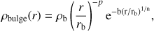 (1)
(1)
where r is the spherical radius and p = 1 − 0.6097/n + 0.05563/n2 yields the Sérsic profile (Prugniel & Simien 1997; Terzić & Graham 2005). For simplicity, the bulge is characterized by a scale velocity, σb, given by![Mathematical equation: $$ \begin{aligned} \sigma _\mathrm{b}=[4\pi n b^{n(p-2)}(n(2-p))r^{2}_\mathrm{b}\rho _\mathrm{b}]^{1/2}. \end{aligned} $$](/articles/aa/full_html/2018/10/aa33509-18/aa33509-18-eq2.gif) (2)
(2)
GalactICs assumes an exponential-sech2 (van der Kruit & Searle 1981) density distribution for the disk: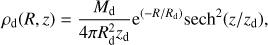 (3)
(3)
where Md is the disk mass, Rd is the disk scale length, and zd is the disk scale height and R is the cylindrical radius. The radial velocity dispersion is given by (4)
(4)
where σ0 and Rσ are the central dispersion and a scale radius respectively. Following Widrow et al. (2008), Rσ is set equal to the scale length based on the observations of Bottema (1993).
However, in terms of the stability, the key value is the Toomre Q parameter calculated at R = 2.2 Rd. Given the use of Rσ = Rd, the variation in σ0 gives only small variations in Q, and therefore of the disk stability. Therefore, for simplicity we fixed σ0 to 90 km s−1. The disk is also truncated at Rt = 50 kpc for all models. The gas disk has an exponential surface density. Following Wang et al. (2010), the disk is initially isothermal, which requires a scale height that increases with radius.
The double power-law halo is defined as (see Widrow et al. 2008)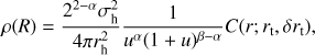 (5)
(5)
where u = r/rh, σh is a scale velocity, and rh is the scale radius. The C(r; rt, δ
rt) term is a truncation factor, given by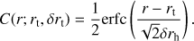 (6)
(6)
In this work the truncation parameters are set to rt = 200 kpc and δrt = 20 kpc
4. Methodology
In this section, we outline the steps adopted to construct the models. The estimation method for the input parameters is outlined in Sect. 4.1 and details about the simulations are given in Sect. 4.2.
Summary of the model parameters.
Comparison between the model input parameters and the THINGS mass model results for NGC 3621.
4.1. Model parameters
In order to find plausible initial conditions for the simulations, we first run a Bayesian analysis for each galaxy. For this analysis we utilize analytic approximations of axisymmetric GalactICs models. In this approximation, the gas disk is given a constant scale height, rather than the flaring profile built into GalactICs. The models are constrained by the RC, the azimuthally averaged 3.6 μm stellar surface brightness, and the gas surface density. In order to avoid any systematic errors caused by the presence of the bars in NGC 1530 and NGC 1300, we fitted only the portion of the RC beyond two bar lengths, Rbar, based on the results of Randriamampandry et al. (2016). We also excluded 3.6 μm data beyond the optical radius defined by R25. Beyond this radius, contamination from the sky background as well as foreground sources affects the surface brightness profile, flattening its slope.
The log-likelihood for a particular model is![Mathematical equation: $$ \begin{aligned} \mathcal L (D|{\Theta })=-\frac{1}{2}\sum ^{N}_{i=1}\left[ \ln \left(2\pi \sigma _\mathrm{D,i}^{2}\right)+\left(\frac{(D_\mathrm{i}-M({\Theta })_\mathrm{i})^{2}}{\sigma ^{2}_\mathrm{D,i}}\right)\right], \end{aligned} $$](/articles/aa/full_html/2018/10/aa33509-18/aa33509-18-eq7.gif) (7)
(7)
where Θ are the model parameters, Di are the observations, σD,i are the uncertainties in the observations, M(Θ)i are the mock observations from the model, and N is the number of observed data points. The posterior probability for a model is (8)
(8)
where p(Θ|I) is the prior probability for a model and Z is the evidence. Since we are performing a parameter estimate, the evidence is simply a normalization factor that is canceled out in the analysis.
To explore the parameter space we used the EMCEE algorithm (Foreman-Mackey et al. 2013). EMCEE is a parallel, affine-invariant Markov Chain Monte Carlo (MCMC) algorithm. It operates by initializing an ensemble of walkers randomly throughout the parameter space. The walkers move throughout the space by first proposing a new position using stretches along the vector to another randomly selected walker. The posterior of the proposal is evaluated and compared to the current posterior in order to determine whether the walker will move or not. In this work, we used 200 walkers for 3500 steps, giving a total of 7 × 10⁵ likelihood calls. For simplicity, the priors for each parameter are uniform. A list of the relevant parameters as well as their minimum and maximum values considered are given in Table 2.
The disk stability can be quantified using the Toomre Q (Toomre 1964) and X (Goldreich & Tremaine 1978, 1979) parameters. The Toomre Q parameter is given by (9)
(9)
for a stellar disk where σr is the radial velocity dispersion at a given radius, κ is the epicyclic frequency, G is the gravitational constant and Σd is the stellar surface density. For the gas disk Qg is (10)
(10)
where cs is the sound speed of the gas and Σg the gas surface density (Wang et al. 2010). It is important to note that Q is a local quantity that depends on the radius. The surface densities, Σ, velocity dispersion σr (given by Eq. (4)), sound speed cs, and the epicyclic frequency κ are all functions of the radius. The Q parameters are measures of a disk’s stability against local perturbations. For this work, we calculate Q at 2.2 Rd as that is where the ratio of disk to halo gravity is maximal. Given our value of σ0 = 90 km s−1 and σr(2.2RD) = 10 km s−1 for all models.
The X parameter is a measure of a disk’s self-gravity and it indicates the disk’s stability against global perturbations. It is given by (11)
(11)
where Vt and Vd are the total circular velocity and the circular velocity due to the disk respectively. As with the Q parameter, it is measured at 2.2 Rd. Unstable disks have large X and low Q, while those with low X and high Q are significantly more stable.
The formal errors obtained during the derivation of the gas surface density and the 3.6 μm surface brightness profiles do not reflect the true uncertainties in the measurements. In order to more accurately represent the uncertainties in these profiles we include two extra parameters; ϵp,G for the gas surface density and ϵp,S for the stellar surface brightness profiles. These are added in quadrature to the formal errors during the Bayesian analysis. For those profiles we set: (12)
(12)
for the gas density and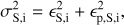 (13)
(13)
for the stellar surface brightness profile, where ϵG,ϵS are the measured uncertainty and ϵp,G, ϵp,G are the error parameters.
The input parameters for the initial condition were selected based on the parameter PDFs and the disk stability parameters PDFs. We selected three models from the PDF for simulation. Model A has a low disk stability, MOdel B uses the peak of the parameter PDFs, and MOdel C has a high degree of stability. For these simulations, we selected the snapshot that best reproduces the observed bar strength and velocity field.
4.2. Numerical simulations
Armed with the GalactICs parameters for each galaxy, we generated our N-body realizations with 106 particles; 5 × 10⁵ for the halo, 2 × 10⁵ for the stellar disk, another 2 × 10⁵ for the gas disk and 105 for the bulge. The models were evolved for five Gyr using the GADGET-2 code with a softening length of 50 pc. Snapshots were taken every 50 Myr in order to follow the evolution of the galaxy in detail. A mock velocity field was calculated for each snapshot and compared to the velocity fields obtained for the actual galaxies.
In detail, the velocity fields for each galaxy were obtained using HI observations of each galaxy combined with position angle, inclination, and systemic velocities listed in Table 1. The mock velocity fields were obtained by rotating and shifting the simulation to the same distance, orientation, and systemic velocity as the actual galaxy and assuming a flat disk model with constant position and inclination angles for all the models. We generated mock velocity maps with the same pixel size and angular resolutions as the observed galaxies. This allowed for a pixel-by-pixel comparison of the model and observed velocity maps. The snapshot that best represents each galaxy was selected based on both the bar strength and this velocity map comparison.
The bar strength of a galaxy can be defined by the amplitude of the Fourier m = 2 mode (see Aguerri et al. 2009; Randriamampandry et al. 2016), which is typically used for N-body simulations. To calculate A2, the surface density of either the stellar or gas disk is expressed as a Fourier series through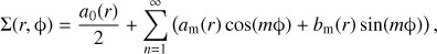 (14)
(14)
where am(r) and bm(r) are the radial Fourier coefficients. The bar strength is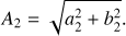 (15)
(15)
We require that both the bar strength and the velocity map of the snapshot match the observations. For the velocity comparison, we first construct a residual map, defined as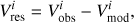 (16)
(16)
where  and
and  are the observed and modeled velocity at a given pixel i in the velocity map. The best-fitting snapshot is the one with the smallest standard deviation σres in the residuals. This quantity is given by
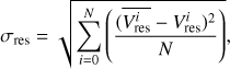 (17)
(17)
where N is the number of pixel and  the mean of the residual velocities.
In addition to these quantities, we also calculated the expected circular velocity curve for each snapshot and a Fourier decomposition of the radial and tangential gas particle velocities. These quantities are used to compare our results to those obtained using ROTCUR and DiskFit.
The “expected” circular velocity curve is defined as (18)
(18)
where Fr is the radial force from the particles calculated azimuthally on an angular grid and Φ is the gravitational potential.
The radial and tangential velocity of the gas particles can also be described in terms of Fourier moments. They are![Mathematical equation: $$ \begin{aligned} V_\mathrm{t}(r,\uptheta )=A_{0,\mathrm t}(r)+ \sum _{m=1}^{\infty }A_\mathrm{m,t}(r)\mathrm{cos}[m\uptheta + \uptheta _\mathrm{m,t}(r)], \end{aligned} $$](/articles/aa/full_html/2018/10/aa33509-18/aa33509-18-eq22.gif) (19)
(19)
and![Mathematical equation: $$ \begin{aligned} V_\mathrm{r}(r,\uptheta )=A_{0,r}(r) + \sum _{m=1}^{\infty }A_\mathrm{m,r}(r)\mathrm{cos}[m\uptheta + \uptheta _\mathrm{m,r}(r)], \end{aligned} $$](/articles/aa/full_html/2018/10/aa33509-18/aa33509-18-eq23.gif) (20)
(20)
where Am,t(r) and Am,r(r) are the tangential and radial Fourier m th velocity moments respectively and θ, θm,t(r) and θm,r(r) are the angular phases. Describing the velocity fields in terms of Fourier moments allows for a comparison with the non-circular moments found by DiskFit for NGC 1530.
NGC 1530 Model input parameters.
5. Results and discussions
In this section, we compare the bar properties and model velocity maps derived from the simulations with the observations. The results for NGC 3621, NGC 1530 and NGC 1300 are presented and discussed in Sects. 5.1–5.3 respectively.
5.1. NGC 3621
The Bayesian analysis of the RC, 3.6 μm surface brightness, and gas surface density of NGC 3621 gives the posterior distribution function (PDF) for the full model parameter space. The best fit GalactICs parameters are given in Table 3 where the uncertainties are the 1-σ error obtained from the PDFs. Using the parameter PDFs we obtained the PDFs of the RC, surface density, and surface brightness profiles shown in Fig. 1, as well as PDFs of the stability parameters. The bulge and disk mass-to-light ratio were also fitted in addition to the GalactICs parameters and the best fit results are given in Table 3. Our best fit result for the disk mass-to-light ratio is consistent with de Blok et al. (2008) if it is compared with their mass-to-light ratio obtained using the Kroupa IMF but two times smaller than their mass-to-light ratio measured using the diet Selpeter IMF. While our model has a smaller disk mass, we also have a bulge component. Furthermore, the sum of the stellar mass is consistent with the de Blok et al. (2008) results.
Finally, Table 3 also shows the parameters of both the NFW and ISO halo models from de Blok et al. (2008) for comparison. However, our analysis excludes both cored and cuspy halos, preferring an inner slope of 0.5. A better comparison of the halo slopes is to the results of Chemin et al. (2011), who uses Einasto profiles (Einasto 1969, 1968, 1965) to model the dark halo of THINGS galaxies. Like the double power-law profile, the Einasto profile also allows for cored and cuspy halos. Using a diet-Saltpeter IMF, Chemin et al. (2011) found an inner slope of 0.53, which is consistent with our PDF. In addition, our inferred gas mass is slightly larger than the THINGS gas mass (see Walter et al. 2008), but this difference is largely due to the different methodologies adopted. The THINGS analysis sums up the mass of all visible gas, while we fit an exponential surface density where Mg is the total integrated mass of that exponential. Nonetheless, Fig. 1 shows that our model provides good fits to the data and is comparable with both the NFW and ISO models of de Blok et al. (2008; see Fig. 4).
While NGC 3621 is classified as an unbarred galaxy, it is unclear which models will form bars a priori. Therefore we selected three models with different disk stability parameters. This selection allowed for a brief exploration of the parameter space. These models (A, B, and C) are listed in Table 3 and plotted in Fig. 1. Model A has the smallest disk/halo ratio, which should give it the most stability against bar formation. Model B correspond to the peak of the parameters PDFs and Model-C is the least stable. After evolving the model for five Gyr, we extracted the stellar surface density and gaseous velocity maps for every snapshot. At each time-step we calculated both the bar strength and the standard deviation of the difference between the simulated and observed velocity maps, which are shown in the left panels of Fig. 2. The standard deviation is obtained first by re-centering and re-aligning the model and observed velocity fields using the GIPSY task TRANSFORM. Then a pixel-by-pixel comparison is performed using the GIPSY utility task SUB. The variation of the likelihood is also shown on the bottom left panel of Fig. 2. The likelihood is given by Eq. (7), except Oi is the observed MOMENT1 map, MD,i the model velocity fields and σD,i the observed MOMENT2 map, which is adopted as the velocity field uncertainties. While we do not define our best-fitting model by the likelihood, it does provide confirmation that our residual method selects the best fitting snapshot from the set of simulations. The right-hand panel of Fig. 2 shows the histogram of the residuals from the best-fitting snapshot. The left-hand panels shows that Model A has the weakest bar at all time steps, and at T = 2 Gyr, it has the lowest standard deviation of all models. At that same time step, the likelihood is maximized.
Figure 3 shows the comparison of the selected snapshot with the observed maps. NGC 3621 exhibits a strong warp in the outermost regions. Unfortunately our simulations are unable to generate warps at this time, so we exclude that region from our analysis and have focused on matching the central, axisymmetric portions of the galaxy. Nonetheless, our method succeeds at our goal of modeling the central portions of the disk, obtaining residuals in the innermost regions of ±10 km s−1. While the velocity maps show a good fit for the model, it is clear that there are differences between the mom0 image and our simulated gas density. This is due to our simulations using an exponential gas disk that cannot reproduce the central holes observed in the HI disk.
It is interesting to note that Model-A is a high stability model, not the model found at the peak of the parameter PDFs. This result emphasizes the importance of running numerical simulations as the Bayesian PDFs include model that rapidly form moderate bars. While these initial conditions are acceptable for the axisymmetric Bayesian analysis, they must be rejected based on the simulations.
Figure 4 shows a comparison of the ROTCUR RC with the THINGS model RCs and the expected circular velocity curve calculated from our best fitting snapshot. These RCs are all consistent with the ROTCUR RC. Interestingly, the simulated RC seems to match the ROTCUR inner 5 kpc slightly better than the THINGS RCs, but it is also slightly below the ROTCUR results in the outermost regions. However, our goal is not to match the RC, but to match the observed velocity map. Nonetheless, our analysis of NGC 3621 is at least as accurate as ROTCUR and other standard methods at recovering the RC for an axisymmetric model. As an added bonus, our RC is built from the underlying mass model, so we do not need to perform an additional inference to recover the dark halo profile.
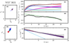 |
Fig. 1. Left panels: PDFs of the disk stability parameters, Q and X. Panel a is for the gas disk, while panel b is for the stellar disk. The stability parameters for the selected models are plotted on I where Model-A is shown as blue diamond, Model-B as cyan star and Model-C as red square. Right panels: PDFs of the RCs (panel c), gas surface density (panel d) and 3.6 μ surface brightness profile (panel e). The best fit to the data is shown as red lines, the stellar disk is shown as dark blue, the green lines are the gas disk contribution, the magenta line is the halo contribution and the light blue lines are the bulge component. The shaded area shows the 1-σ error and the data are shown as black points. |
NGC 1300 Model input parameters.
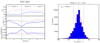 |
Fig. 2. Left panels: variation of the bar strength A2 as function of the epoch is shown on the top panel, the standard deviation of the residual σres on the middle and the variation of the likelihood. The vertical dashed line indicates the epoch of the selected snapshot. Right panel: histogram of the residuals for Model-A at T = 2.0 Gyr, the red line is the best fit to the data and σres is the standard deviation of the residuals. The vertical dashed lines indicate the mean and standard deviation of the residuals. |
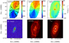 |
Fig. 3. Observed and simulated maps for NGC 3621, Model-A at T = 2 Gyr: the moment-1, model velocity field and residual maps are presented on the top panels. The black contours are spaced by 50 km s−1. The near-infrared K-band image from Jarrett et al. (2003; it is important to note that this is not used in any analysis, but to show the corresponding stellar systems to the gas maps that are used for the analysis) is shown with the moment-0 and the simulated gas surface density maps on the bottom panels. The moment1 and moment0 maps are obtained from the THINGS database (http://www.mpia.de/THINGS/Data.html). |
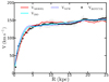 |
Fig. 4. Comparison between the observed RC, the RC calculated from the gravitational potential with the ISO and NFW mass model results from de Blok et al. (2008) for the NGC 3621-A at T = 2.0 Gyr. |
5.2. NGC 1530
NGC 1530 provides an excellent case for comparing our method with DiskFit as it has a strong bar at an intermediate angle. The best fit results from the initial Bayesian analysis are presented in Table 4 while Fig. 5 shows the model stability and the comparison to the observations. In this case we avoided the barred regions of the galaxy for the Bayesian analysis in the RC and surface density fits while we avoid the outer regions of the 3.6 μm surface profile due to possible contamination.
As with NGC 3621, we simulated three models that represent the parameter space. These models correspond to low and high disk stabilities and the peak of the parameter PDFs. The initial conditions for the simulation are listed in Table 4. We analyzed each snapshot, comparing both the bar strength, the standard deviation of the velocity residuals and the likelihood for each model, which is shown in the left panels of Fig. 6. We then selected the model and snapshot that not only reproduces the bar strength but also has the lowest standard deviation of the residual. One key issue with NGC 1530 that is question of the bar orientation. The K band image has the optical bar oriented at −25 deg. However, the mom0 gas map shows a double-bar structure with the inner bar oriented along the stellar bar, but the outer bar is at −35 deg. We explored a number of model orientations and find the best results when we align the model with the outer gas bar.
The evolution of the bar strength and residuals shown in Fig. 6 demonstrates a number of interesting points. Model C shows rapid bar growth until it buckles at T ∼ 0.8 Gyr and decreases to a constant value. Interestingly the minima of Model C does not occur when it has the correct bar strength. On the other hand, Model A never grows a bar that is as strong as the observed bar of NGC 1530. Only Model B has a minima when it matches the bar strength. This minima is also the global minima, meaning that the snapshot of Model B at T = 2 .5 Gyr is our selected model. As shown in the right-hand panel of Fig. 6, this snapshot has standard deviation σres = 9 km s−1.
Figure 7 shows the comparison of this snapshot to observations of the system. The largest residuals occur near the center of the velocity field. However, the mom0 map shows a greater degree of structure than is seen in the K-band image. This additional structure may explain some of the residual structure seen in Fig. 7. To fully explore this issue, additional simulations will be required.
The residual map obtain from DiskFit analysis of the same velocity map shown in Fig. 8 is comparable to our method, even though DiskFit is explicitly designed to match velocity maps of galaxies like NGC 1530. Furthermore, as shown in the lower left panel of Fig. 8, our inferred RC and non-axisymmetric motions agree with those obtained by the DiskFit analysis. While DiskFit is designed to reproduce the velocity maps of barred galaxies, our results remain comparable. Moreover, we can apply our method to galaxies like NGC 1300 and, as mentioned earlier, our method gives a full mass model.
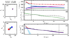 |
Fig. 5. Same as in Fig. 1 but for NGC 1530. The vertical dashed lines indicate regions that are excluded from our analysis due to the presence of the bar (RC and gas SD) or possible contamination (surface brightness). |
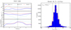 |
Fig. 6. Same as Fig. 2 for NGC 1530. The dashed horizontal line is the A2 from Aguerri et al. (1998). The vertical dashed line indicates the location of the selected snapshot. |
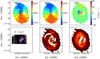 |
Fig. 7. Simulated and observed maps for NGC 1530, Model-B. The panels are the same as in Fig. 3. The black contours are spaced by 50 km s−1. The near-infrared K-band image is taken from Regan et al. (1995). |
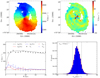 |
Fig. 8. DiskFit results for NGC 1530. The moment1 map is on the top left panel and the residual map is displayed on the top right panel. A histogram of the residuals is presented on the bottom right panel and a comparison between the DiskFit velocities Vt, V2t and V2r with the amplitude of the m = 0 and m = 2 Fourier mode A0 and A2 on the left panel. The black contours are spaced by 50 km s−1. |
5.3. NGC 1300
NGC 1300 is the perfect galaxy for this method of tailored numerical simulations. It has a strong bar aligned with the major axis, which means that ROTCUR will underestimate the RC of this galaxy (see Randriamampandry et al. 2016) and, due to degeneracies in the fitting formula, DiskFit will fail (Sellwood & Sánchez 2010). As with the other galaxies, we began with a Bayesian analysis of the RC, 3.6 μ surface brightness, and surface density. To avoid complications due to the bar, we excluded data from the RC and the gas surface density from the inner 6 kpc. The best fit parameters are given in Table 5. The stability PDFs and observation comparisons are shown in Fig. 9. This analysis suggests that NGC 1300 has a halo that is more cuspy than cored.
Following our general methodology, the input parameters for the three models, namely A, B, and C are selected based on their disk stability and listed in Table 5. We examine the snapshots from our simulations that have the same bar strength as reported in Díaz-García et al. (2016) and the minimum residual velocity standard deviation. Figure 10 shows that each of the simulations reach the desired bar strength over different time scales. However, when Model A reaches the target bar strength at T = 3.5 Gyr it also has the smallest residual with σres = 9 km s−1. This is also the best representation of NGC 1300 according to the likelihood plot shown on the bottom panel of Fig. 10. The comparison of the best-fitting snapshot to the actual observations is shown in Fig. 11. It is clear that our methodology can be applied to bars that are aligned with the major axis of the galaxy. And, for the first time, we produced a mass model for NGC 1300. To illustrate the strength of our method, we compared the RC derived by ROTCUR to the expected circular velocity curve from the simulation. As shown in the upper panel of Fig. 12, there is a significant difference between these two RCs, with the ROTCUR curve underestimating the velocity in the inner 10 kpc. The lower panel of Fig. 12 shows the mass profile inferred from the ROTCUR RC compared to the true mass profile of the galaxy. There is a significant difference between these two mass profiles, which will lead to radically different inferences of the DM content of NGC 1300. This emphasizes the importance of correcting RC of barred galaxies for the non-circular motions induced by a bar before using them for mass model purposes.
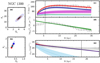 |
Fig. 9. Same as in Fig. 1 for NGC 1300, the vertical dashed delineate the part of data used in the fit. |
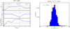 |
Fig. 10. Same as Fig. 2 for NGC 1300. The dashed horizontal line is the A2 from Díaz-García et al. (2016). The vertical dashed line indicates the location of the selected snapshot. |
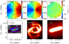 |
Fig. 11. Simulated and observed maps for NGC 1300, Model-A. The panels are the same as in Fig. 3. The black contours are spaced by 50 km s−1. The near-infrared K-band image is taken from Jarrett et al. (2003). |
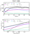 |
Fig. 12. RC measured with ROTCUR is compared with the expected velocities from the gravitational force. The mass profile inferred from the ROTCUR RC and the expected mass from the snapshot are presented on the bottom panel where the black points are the ROTCUR RC, the expected velocities and mass are shown as black lines, the stellar disk is shown as dashed blue, the green dashed line is the gas disk contribution, the magenta line is the halo contribution, the cyan line the bulge component and the dashed black line on the bottom panel is the mass profile inferred from the ROTCUR RC. |
6. Summary and conclusions
We presented a two-step method to study the mass distribution of strongly barred galaxies using numerical simulations. An initial Bayesian analysis was performed on the azimuthally averaged RC, 3.6 μm surface brightness, and gas surface density. The PDFs from the Bayesian analysis were combined with an examination of the resulting disk stability to determine the initial conditions. This method is suitable for barred galaxies with a bar that is parallel to one of the symmetry axes or when the RC derived using conventional method is not reliable to derive the mass distribution. The N-body systems were initialized using a new version of the GalactICS code and evolved for five Gyrs using the GADGET-2 code (Springel 2005). The best fitting snapshot is found by comparing the bar properties and velocity maps of the simulation to observations of the galaxy..
We applied this algorithm to NGC 3621, 1530, and 1300. For NGC 3621 we found that our model is consistent with the ISO and NFW results from de Blok et al. (2008) and the Einasto model from Chemin et al. (2011). It also reproduced the overall shape of the observed RC especially in the inner five kpc of the RC. Our result showed that the peak of the parameter PDFs does not always reproduce the actual galaxy. This is why simulations are necessary in addition to the Bayesian analysis. The Bayesian analysis allowed us to find plausible axisymmetric models to use for the simulation initial conditions. But it was the simulations that showed us whether those models will produce bars and 2D velocity maps like those observed.
We were able to reproduce the bar strength from Aguerri et al. (1998) and the kinematic structure of NGC 1530. Our result is comparable to the DiskFit analysis despite DiskFit being designed to reproduce the velocity map of galaxies with intermediate bar orientation, and, our azimuthally averaged velocities as well as the radial and tangential velocity moments agree with the results from DiskFit.
Since NGC 1300 is a strongly barred galaxy where the bar is parallel to its position angle, algorithms like DiskFit cannot recover the RC from the velocity map (Sellwood & Sánchez 2010; Randriamampandry et al. 2016). Similarly, ROTCUR underestimates the RC for galaxies with such a bar orientation (Randriamampandry et al. 2015). Our method is not subject to these same restrictions. Our results showed that the mass profile derived from ROTCUR largely underestimates the dynamical mass. This shows the importance of correcting the RC of barred galaxies before using them for mass models analysis.
This method, while successful in modeling NGC 1300, is not meant to be a replacement algorithm for DiskFit. Rather, it is a complementary approach that can be applied to galaxies where algorithms such as DiskFit fails. Based on the results of Randriamampandry et al. (2016), this occurs when bars are within approximately ten degrees of the major or minor axes. Given the frequency of barred galaxies and assuming random orientations, these limits imply that there are many galaxies that would benefit from such an analysis.
In its current state, this algorithm produces viable mass models for specific galaxies. To get the “true” mass distribution, we must extend this algorithm to a representative grid of simulations rather than selecting three interesting models. Such a grid will allow for a test of the uniqueness of our solutions. Related to this issue is the impact of the inferred stellar parameters on the results. While our mass-to-light ratios are consistent with those assuming Saltpeter (NGC 1530) and Kroupa (NGC 1300) IMFs, in the future we wish to include these directly into our modeling. We also wish to extend the method to utilize fits to data cubes rather than velocity maps.
Acknowledgments
We thank the anonymous referee for constructive comments. CC’s work is based upon research supported by the South African Research Chairs Initiative (SARChI) of the Department of Science and Technology (DST), the SKA SA and the National Research Foundation (NRF). ND and THR’s work were supported by a SARChI’s South African SKA Fellowship. LMW is supported by the Natural Sciences and Engineering Research Council of Canada through Discovery Grants.
References
- Aguerri, J. A. L., Beckman, J. E., & Prieto, M. 1998, AJ, 116, 2136 [Google Scholar]
- Aguerri, J. A. L., Muñoz-Tuñón, C., Varela, A. M., & Prieto, M. 2000, A&A, 361, 841 [NASA ADS] [Google Scholar]
- Aguerri, J. A. L., Méndez-Abreu, J., & Corsini, E. M. 2009, A&A, 495, 491 [NASA ADS] [CrossRef] [EDP Sciences] [Google Scholar]
- Athanassoula, E. 2002, Ap&SS, 281, 39 [NASA ADS] [CrossRef] [Google Scholar]
- Athanassoula, E., & Bureau, M. 1999, ApJ, 522, 699 [NASA ADS] [CrossRef] [Google Scholar]
- Athanassoula, E., & Misiriotis, A. 2002, MNRAS, 330, 35 [NASA ADS] [CrossRef] [Google Scholar]
- Athanassoula, E., Machado, R. E. G., & Rodionov, S. A. 2013, MNRAS, 429, 1949 [NASA ADS] [CrossRef] [Google Scholar]
- Begeman, K. G. 1989, A&A, 223, 47 [NASA ADS] [Google Scholar]
- Bershady, M. A., Verheijen, M. A. W., Swaters, R. A., et al. 2010, ApJ, 716, 198 [NASA ADS] [CrossRef] [Google Scholar]
- Bonnarel, F., Boulesteix, J., Georgelin, Y. P., et al. 1988, A&A, 189, 59 [NASA ADS] [Google Scholar]
- Bosma, A. 1978, PhD Thesis, Groningen Univ., The Netherlands [Google Scholar]
- Bosma, A. 1981, AJ, 86, 1825 [NASA ADS] [CrossRef] [Google Scholar]
- Bosma, A., Ekers, R. D., & Lequeux, J. 1977a, A&A, 57, 97 [NASA ADS] [Google Scholar]
- Bosma, A., van der Hulst, J. M., & Sullivan, W. T., III 1977b, A&A, 57, 373 [NASA ADS] [Google Scholar]
- Bottema, R. 1993, A&A, 275, 16 [NASA ADS] [Google Scholar]
- Chemin, L., de Blok, W. J. G., & Mamon, G. A. 2011, AJ, 142, 109 [NASA ADS] [CrossRef] [Google Scholar]
- Chequers, M. H., Spekkens, K., Widrow, L. M., & Gilhuly, C. 2016, MNRAS, 463, 1751 [NASA ADS] [CrossRef] [Google Scholar]
- Condon, J. J., Helou, G., Sanders, D. B., & Soifer, B. T. 1996, ApJS, 103, 81 [NASA ADS] [CrossRef] [Google Scholar]
- de Blok, W. J. G., Walter, F., Brinks, E., et al. 2008, AJ, 136, 2648 [NASA ADS] [CrossRef] [Google Scholar]
- de Vaucouleurs, G., & Peters, W. L. 1981, ApJ, 248, 395 [NASA ADS] [CrossRef] [Google Scholar]
- de Vaucouleurs, G., de Vaucouleurs, A., Corwin, H. G. Jr., et al. 1991, Third Reference Catalogue of Bright Galaxies (New York, NY: Springer) [Google Scholar]
- Díaz-García, S., Salo, H., Laurikainen, E., & Herrera-Endoqui, M. 2016, A&A, 587, A160 [NASA ADS] [CrossRef] [EDP Sciences] [Google Scholar]
- Dicaire, I., Carignan, C., Amram, P., et al. 2008, MNRAS, 385, 553 [NASA ADS] [CrossRef] [Google Scholar]
- Duval, M. F., & Athanassoula, E. 1983, A&A, 121, 297 [NASA ADS] [Google Scholar]
- Einasto, J. 1965, Trudy Astrofizicheskogo Instituta Alma-Ata, 5, 87 [NASA ADS] [Google Scholar]
- Einasto, J. 1968, Publications of the Tartu Astrofizica Observatory, 36, 414 [Google Scholar]
- Einasto, J. 1969, Astron. Nachr., 291, 97 [NASA ADS] [CrossRef] [Google Scholar]
- England, M. N. 1989, ApJ, 337, 191 [NASA ADS] [CrossRef] [Google Scholar]
- Freedman, W. L., Madore, B. F., Gibson, B. K., et al. 2001, ApJ, 553, 47 [NASA ADS] [CrossRef] [Google Scholar]
- Foreman-Mackey, D., Hogg, D. W., Lang, D., & Goodman, J. 2013, PASP, 125, 306 [CrossRef] [Google Scholar]
- Gentile, G., Famaey, B., & de Blok, W. J. G. 2011, A&A, 527, A76 [NASA ADS] [CrossRef] [EDP Sciences] [Google Scholar]
- Goldreich, P., & Tremaine, S. 1978, ApJ, 222, 850 [NASA ADS] [CrossRef] [Google Scholar]
- Goldreich, P., & Tremaine, S. 1979, ApJ, 233, 857 [NASA ADS] [CrossRef] [MathSciNet] [Google Scholar]
- Jarrett, T. H., Chester, T., Cutri, R., Schneider, S. E., & Huchra, J. P. 2003, AJ, 125, 525 [NASA ADS] [CrossRef] [Google Scholar]
- Kormendy, J. 1983, ApJ, 275, 529 [NASA ADS] [CrossRef] [Google Scholar]
- Kuijken, K., & Dubinski, J. 1995, MNRAS, 277, 1341 [CrossRef] [Google Scholar]
- Kuzio de Naray, R., Arsenault, C. A., Spekkens, K., et al. 2012, MNRAS, 427, 2523 [NASA ADS] [CrossRef] [Google Scholar]
- Laurikainen, E., Salo, H., & Buta, R. 2004, ApJ, 607, 103 [NASA ADS] [CrossRef] [Google Scholar]
- Lindblad, P. A. B., Lindblad, P. O., & Athanassoula, E. 1996, A&A, 313, 65 [NASA ADS] [Google Scholar]
- Lindblad, P. A. B., Kristen, H., Joersaeter, S., & Hoegbom, J. 1997, A&A, 317, 36 [NASA ADS] [Google Scholar]
- Lütticke, R., Dettmar, R.-J., & Pohlen, M. 2000, A&A, 362, 435 [NASA ADS] [Google Scholar]
- Martinsson, T. P. K. 2011, PhD Thesis, Groningen Univ., The Netherlands [Google Scholar]
- Menéndez-Delmestre, K., Sheth, K., Schinnerer, E., Jarrett, T. H., & Scoville, N. Z. 2007, ApJ, 657, 790 [NASA ADS] [CrossRef] [Google Scholar]
- Oh, S.-H., de Blok, W. J. G., Walter, F., Brinks, E., & Kennicutt, R. C., Jr 2008, AJ, 136, 2761 [NASA ADS] [CrossRef] [Google Scholar]
- Ohta, K., Hamabe, M., & Wakamatsu, K.-I. 1990, ApJ, 357, 71 [NASA ADS] [CrossRef] [Google Scholar]
- Pfenniger, D., & Friedli, D. 1991, A&A, 252, 75 [NASA ADS] [Google Scholar]
- Prugniel, P., & Simien, F. 1997, A&A, 321, 111 [NASA ADS] [Google Scholar]
- Puglielli, D., Widrow, L. M., & Courteau, S. 2010, ApJ, 715, 1152 [NASA ADS] [CrossRef] [Google Scholar]
- Randriamampandry, T. H., Combes, F., Carignan, C., & Deg, N. 2015, MNRAS, 454, 3743 [NASA ADS] [CrossRef] [Google Scholar]
- Randriamampandry, T. H., Deg, N., Carignan, C., Combes, F., & Spekkens, K. 2016, A&A, 594, A86 [NASA ADS] [CrossRef] [EDP Sciences] [Google Scholar]
- Regan, M. W., Vogel, S. N., & Teuben, P. J. 1995, ApJ, 449, 576 [NASA ADS] [CrossRef] [Google Scholar]
- Rogstad, D. H., Lockhart, I. A., & Wright, M. C. H. 1974, ApJ, 193, 309 [NASA ADS] [CrossRef] [Google Scholar]
- Salo, H. 1991, A&A, 243, 118 [NASA ADS] [Google Scholar]
- Sellwood, J. A., & Sánchez, R. Z. 2010, MNRAS, 404, 1733 [NASA ADS] [Google Scholar]
- Sorce, J. G., Tully, R. B., Courtois, H. M., et al. 2014, MNRAS, 444, 527 [Google Scholar]
- Spekkens, K., & Sellwood, J. A. 2007, ApJ, 664, 204 [NASA ADS] [CrossRef] [Google Scholar]
- Springel, V. 2005, MNRAS, 364, 1105 [NASA ADS] [CrossRef] [Google Scholar]
- Springob, C. M., Masters, K. L., Haynes, M. P., Giovanelli, R., & Marinoni, C. 2009, ApJS, 182, 474 [NASA ADS] [CrossRef] [Google Scholar]
- Taranu, D. S., Obreschkow, D., Dubinski, J., et al. 2017, ApJ, 850, 70 [NASA ADS] [CrossRef] [Google Scholar]
- Terzić, B., & Graham, A. W. 2005, MNRAS, 362, 197 [NASA ADS] [CrossRef] [Google Scholar]
- Teuben, P. J., Sanders, R. H., Atherton, P. D., & van Albada, G. D. 1986, MNRAS, 221, 1 [NASA ADS] [CrossRef] [Google Scholar]
- Toomre, A. 1964, ApJ, 139, 1217 [NASA ADS] [CrossRef] [Google Scholar]
- van Albada, G. D. 1980, A&A, 90, 123 [Google Scholar]
- van der Kruit, P. C., & Searle, L. 1981, A&A, 95, 105 [NASA ADS] [Google Scholar]
- Walter, F., Brinks, E., de Blok, W. J. G., et al. 2008, AJ, 136, 2563 [NASA ADS] [CrossRef] [Google Scholar]
- Wang, H.-H., Klessen, R. S., Dullemond, C. P., van den Bosch, F. C., & Fuchs, B. 2010, MNRAS, 407, 705 [NASA ADS] [CrossRef] [Google Scholar]
- Widrow, L. M., Pym, B., & Dubinski, J. 2008, ApJ, 679, 1239 [NASA ADS] [CrossRef] [Google Scholar]
- Zánmar Sánchez, R., Sellwood, J. A., Weiner, B. J., & Williams, T. B. 2008, ApJ, 674, 797 [NASA ADS] [CrossRef] [Google Scholar]
- Zurita, A., Relaño, M., Beckman, J. E., & Knapen, J. H. 2004, A&A, 413, 73 [NASA ADS] [CrossRef] [EDP Sciences] [Google Scholar]
Appendix A:
PDF of the model parameters
The one and two dimensional PDFs for nine of the free parameters are shown in Figs. A.1–A.3 for NGC 3621, NGC 1530 and NGC 1300 respectively. We do not show the scale heights for the stellar and gas disks, as the stellar scale height is poorly constrained, and the GalactICS gas disk has a varying scale height determined by the kinematic gas temperature. These figures show that the gas parameters are more tightly constrained than the bulge, disk, and halo parameters. There are a number of correlations apparent between the parameters. Galaxies with larger sigma prefer smaller alpha and larger beta. Additionally, there is a correlation between σh and Md that shows the classic disk -halo degeneracy.
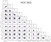 |
Fig. A.1. Two-dimensional and one-dimensional PDFs of the model parameters for NGC 3621: the two-dimensional PDFs are shown on the lower triangular of the matrix and the one-dimensional PDFs on the principal diagonals. The red and blue contour in each panel delineates the 68% and 95% confidence levels. The cyan stars correspond to Model-C, the blue diamonds to Model-A and the red square to Model-B. |
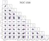 |
Fig. A.2. Two-dimensional and one-dimensional PDFs of the model parameters for NGC 1530. Lines and symbols are the same as in Fig. A.1. |
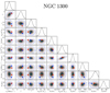 |
Fig. A.3. Two-dimensional and one-dimensional PDFs of the model parameters for NGC 1300. Lines and symbols are the same as in Fig. A.1 |
All Tables
Comparison between the model input parameters and the THINGS mass model results for NGC 3621.
All Figures
|
Fig. 1. Left panels: PDFs of the disk stability parameters, Q and X. Panel a is for the gas disk, while panel b is for the stellar disk. The stability parameters for the selected models are plotted on I where Model-A is shown as blue diamond, Model-B as cyan star and Model-C as red square. Right panels: PDFs of the RCs (panel c), gas surface density (panel d) and 3.6 μ surface brightness profile (panel e). The best fit to the data is shown as red lines, the stellar disk is shown as dark blue, the green lines are the gas disk contribution, the magenta line is the halo contribution and the light blue lines are the bulge component. The shaded area shows the 1-σ error and the data are shown as black points. |
| In the text | |
|
Fig. 2. Left panels: variation of the bar strength A2 as function of the epoch is shown on the top panel, the standard deviation of the residual σres on the middle and the variation of the likelihood. The vertical dashed line indicates the epoch of the selected snapshot. Right panel: histogram of the residuals for Model-A at T = 2.0 Gyr, the red line is the best fit to the data and σres is the standard deviation of the residuals. The vertical dashed lines indicate the mean and standard deviation of the residuals. |
| In the text | |
|
Fig. 3. Observed and simulated maps for NGC 3621, Model-A at T = 2 Gyr: the moment-1, model velocity field and residual maps are presented on the top panels. The black contours are spaced by 50 km s−1. The near-infrared K-band image from Jarrett et al. (2003; it is important to note that this is not used in any analysis, but to show the corresponding stellar systems to the gas maps that are used for the analysis) is shown with the moment-0 and the simulated gas surface density maps on the bottom panels. The moment1 and moment0 maps are obtained from the THINGS database (http://www.mpia.de/THINGS/Data.html). |
| In the text | |
|
Fig. 4. Comparison between the observed RC, the RC calculated from the gravitational potential with the ISO and NFW mass model results from de Blok et al. (2008) for the NGC 3621-A at T = 2.0 Gyr. |
| In the text | |
|
Fig. 5. Same as in Fig. 1 but for NGC 1530. The vertical dashed lines indicate regions that are excluded from our analysis due to the presence of the bar (RC and gas SD) or possible contamination (surface brightness). |
| In the text | |
|
Fig. 6. Same as Fig. 2 for NGC 1530. The dashed horizontal line is the A2 from Aguerri et al. (1998). The vertical dashed line indicates the location of the selected snapshot. |
| In the text | |
|
Fig. 7. Simulated and observed maps for NGC 1530, Model-B. The panels are the same as in Fig. 3. The black contours are spaced by 50 km s−1. The near-infrared K-band image is taken from Regan et al. (1995). |
| In the text | |
|
Fig. 8. DiskFit results for NGC 1530. The moment1 map is on the top left panel and the residual map is displayed on the top right panel. A histogram of the residuals is presented on the bottom right panel and a comparison between the DiskFit velocities Vt, V2t and V2r with the amplitude of the m = 0 and m = 2 Fourier mode A0 and A2 on the left panel. The black contours are spaced by 50 km s−1. |
| In the text | |
|
Fig. 9. Same as in Fig. 1 for NGC 1300, the vertical dashed delineate the part of data used in the fit. |
| In the text | |
|
Fig. 10. Same as Fig. 2 for NGC 1300. The dashed horizontal line is the A2 from Díaz-García et al. (2016). The vertical dashed line indicates the location of the selected snapshot. |
| In the text | |
|
Fig. 11. Simulated and observed maps for NGC 1300, Model-A. The panels are the same as in Fig. 3. The black contours are spaced by 50 km s−1. The near-infrared K-band image is taken from Jarrett et al. (2003). |
| In the text | |
|
Fig. 12. RC measured with ROTCUR is compared with the expected velocities from the gravitational force. The mass profile inferred from the ROTCUR RC and the expected mass from the snapshot are presented on the bottom panel where the black points are the ROTCUR RC, the expected velocities and mass are shown as black lines, the stellar disk is shown as dashed blue, the green dashed line is the gas disk contribution, the magenta line is the halo contribution, the cyan line the bulge component and the dashed black line on the bottom panel is the mass profile inferred from the ROTCUR RC. |
| In the text | |
|
Fig. A.1. Two-dimensional and one-dimensional PDFs of the model parameters for NGC 3621: the two-dimensional PDFs are shown on the lower triangular of the matrix and the one-dimensional PDFs on the principal diagonals. The red and blue contour in each panel delineates the 68% and 95% confidence levels. The cyan stars correspond to Model-C, the blue diamonds to Model-A and the red square to Model-B. |
| In the text | |
|
Fig. A.2. Two-dimensional and one-dimensional PDFs of the model parameters for NGC 1530. Lines and symbols are the same as in Fig. A.1. |
| In the text | |
|
Fig. A.3. Two-dimensional and one-dimensional PDFs of the model parameters for NGC 1300. Lines and symbols are the same as in Fig. A.1 |
| In the text | |
Current usage metrics show cumulative count of Article Views (full-text article views including HTML views, PDF and ePub downloads, according to the available data) and Abstracts Views on Vision4Press platform.
Data correspond to usage on the plateform after 2015. The current usage metrics is available 48-96 hours after online publication and is updated daily on week days.
Initial download of the metrics may take a while.