© ESO 2018

1. Introduction

Lagrangian coherent structures (LCS), introduced by Haller & Yuan (2000), have been proposed as dynamical replacements for invariant manifolds in the study of the dynamics of non-autonomous systems. They behave as hypersurfaces with maximally attracting or repelling properties and organizing the evolution of the system in a similar way as invariant manifolds do in autonomous problems.

Lagrangian coherent structures have been succesfully employed in the study of fluid dynamics problems (e.g., Farazmand & Haller 2012, 2013), or in the elliptic restricted three-body problem (ER3BP; see Gawlik et al. 2009). The exact concept of what a LCS is, is still evolving. Shadden et al. (2005), Lekien et al. (2007), Gawlik et al. (2009), among others, consider them as ridges of the values of finite-time Lyapunov exponents (FTLE) of the flow, whereas Farazmand & Haller (2012) and therein, Onu et al. (2015), characterize them as critical lines of the averaged material shear, which is an auxiliary autonomous functional also derived from the flow.

We seek to apply the theory of LCS to the study of the non-autonomous version of the precessing galactic bar model (Sánchez-Martín et al. 2016). This model is a Hamiltonian system which in its autonomous version has been studied by means of invariant manifolds. Our goal in this paper is to compare the results provided by the invariant manifolds with those of the LCS in the autonomous version, and furthermore, to study a simple non-autonomous version of this problem. We have developed software to implement the characterization of LCS given by Haller in two dimensions (Onu et al. 2015), such as stretch and strainlines. In the work it is to determine LCS in both autonomous and non-autonomous versions of a precesing galactic bar potential.

Lagrangian coherent structures are a quantitative characterization of chaotic transport, based on the fast dynamical indicator FTLE. In the literature there exist analogous methods to detect chaotic and ordered orbits of a dynamical system, such as the smaller alignment index (SALI; Skokos 2001), or the mean exponential growth factor of nearby orbits (MEGNO; Cincotta et al. 2003). The main idea of the SALI method is to study the evolution in time of two different deviation vectors. In this case, if SALI tends to zero the orbit is chaotic, whereas if it tends to a positive non-zero value the orbit is ordered. The eficiency of the SALI method has been widely proved in well known problems (Skokos et al. 2004) and in barred galaxies models (Manos et al. 2008). The MEGNO method is a refinement of the Lyapunov characteristic number (LCN): the latter studies the mean exponential rate of divergence of nearby orbits by integrating them over a long time span, while MEGNO is a time-weighted version of the LCN which can be found by integrating the perturbed orbits over a shorter time span and still detects the regularity or chaocity of the system, and estimates its hyperbolicity in the latter case. MEGNO has been applied to the study of the dynamics of elliptical galaxies (Cincotta al. 2008), and of planetary systems (Goździewski et al. 2001).

The paper is organized as follows: in Sect. 2 we review the theory concerning LCS and their correspondence with FTLE. Section 3 discusses in detail how to compute LCS in practice. The application of LCS to the galactic model, and their relation with the classical invariant manifolds is shown in Sect. 4. Section 5 presents the conclusions of the paper, and outlines directions for future work in the topic.

2. Lagrangian coherent structures

The starting point to study the local and global structure of a time-dependent flow is the Jacobian given by the variational flow. Let us consider a dynamical system of the form,$$\begin{array}{c}\hfill \dot{\mathbf{x}}=\mathbf{v}(\mathbf{x},t),\mathbf{x}\in U\subset {\mathbb{R}}^n,t\in [a,b],\end{array}$$(1)

where U denotes an open, bounded subset of ℝⁿ, the time t varying over the finite interval [a, b], and v : U × [a, b]→ℝⁿ is a sufficiently smooth vector field. For a ≤ t ₀ < t ≤ b, we define the flow map$$\begin{array}{c}\hfill {\mathbf{F}}_{t_0}^t({\mathbf{x}}_0):=\mathbf{x}(t),\end{array}$$(2)

where x(t) is the solution of Eq. (1) such that x(t₀) = x₀.

For a fixed time t, the Jacobian $\nabla F_{t_0}^t\hspace{0.17em}({\text{x}}_0)$ provides a linearization of the variation of the flow ${\mathbf{F}}_{t_0}^t$ with respect to the initial condition x₀. Its singular value decomposition (SVD) points out the directions where the flow is maximally spread (maximally compressed), with the rate of expansion (compression) given by the singular values of the Jacobian. For instance, the maximal expansion rate of the flow around x₀ is the first singular value of its Jacobian, which is the Euclidean norm¹ of the Jacobian $\left|\right|\nabla F_{t_0}^t\hspace{0.17em}({\text{x}}_0)\left|\right|$ , and the direction where this maximal expansion happens is given by its associated right-singular vector of the SVD.

The SVD of the Jacobian $\nabla F_{t_0}^t\hspace{0.17em}({\text{x}}_0)$ is equivalent to the diagonalization of the Cauchy-Green, or strain, tensor field, widely used in Mechanics:$$\begin{array}{c}\hfill {\mathbf{C}}_{t_0}^t={(\mathrm{\nabla }{\mathbf{F}}_{t_0}^t({\mathbf{x}}_0))}^T\mathrm{\nabla }{\mathbf{F}}_{t_0}^t({\mathbf{x}}_0),\end{array}$$(3)

where T stands for matrix transposition.

The eigenvalues of the Cauchy-Green tensor are the squares of the singular values of the Jacobian, and the eigenvectors of the Cauchy-Green tensor, ξ₁, ξ₂, …,ξ_n, are the right-singular vectors of the Jacobian. In both instances an orthonormal basis of vectors is adopted, but, unfortunately, opposite sorting conventions are followed: It is usual to sort the singular values from largest to smallest, $\left|\right|\nabla F_{t_0}^t\hspace{0.17em}({\text{x}}_0)\left|\right|$ = σ₁ ≥ σ₂ ≥ … ≥ σ_n, while the eigenvalues of the Cauchy-Green tensor are usually labelled in increasing order, λ₁ ≤ λ₂ ≤ … ≤ λ_n . See Golub & Van Loan (2012) for a mathematical discussion of these concepts.

The concept of a LCS is somewhat recent and still work in progress. Several versions with slight differences can be found in the literature. We shall use in this work the definition of LCS given by Haller, and the following characterization of LCS in two dimensions, based on variational theory, from Farazmand & Haller (2012).

A line ℳ(t₀) in the two dimensional spatial domain of the dynamical system is a repelling LCS (or strainline) for the system over the time interval [t₀, t] if and only if, for every point x₀ ∈ ℳ(t₀) the following conditions hold,

1. λ₁(x₀) ≠ λ₂(x₀) > 1;

2. ⟨ξ₂(x₀),∇²λ₂(x₀)ξ₂(x₀)⟩ < 0;

3. ξ₂(x₀) ⊥ ℳ(t₀);

4. ⟨∇λ₂(x₀),ξ₂(x₀) ⟩ = 0,

where λ₁ and λ₂, are respectively the smallest and largest eigenvalues of the Cauchy-Green tensor of the flow, and ξ₁, ξ₂ are the corresponding eigenvector fields. We note that condition (1) ensures that the stretching rate of the flow (i.e. the rate at which particular solutions of the system separate when integrated over the time interval [t₀, t]) is greater along the normal direction that along the tangential direction. Conditions (3) and (4) assure that the normal stretch rate of the flow along the strainline is a local extremum relative to close material lines, while condition (2) assures this extremum as a strict local maximum.

The characterization of an attracting LCS (or stretchline) is analogous to that of a strainline, but replacing the second eigenvalue and vector of the Cauchy-Green tensor by the first ones, and reversing the inequality in condition (2) above.

For a dynamical system close to being autonomous, in the neighbourhood of a hyperbolic equilibrium point the repelling LCS are the indicator analogue of stable invariant manifolds, while attracting LCS are the analogue of unstable invariant manifolds. The reason for this is illustrated by Fig. 1: a segment of initial conditions transverse to the stable manifold will stretch to a great extent when integrated beyond the equilibrium point, while a segment of initial conditions transverse to the unstable manifold will be greatly compressed by the flow. Both these stretchings and compressions are the greatest taking place in the neighbourhood of the equilibrium point.

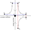Fig. 1. Neighbourhood of a hyperbolic equilibrium point in a two-dimensional, autonomous, dynamical system: The blue segment of initial conditions from Q0 to R0, transverse to the stable invariant manifold, will undergo great stretch when the system is integrated from time t0 to tf and it transforms into the curve from Qf to Rf. Conversely, the red segment of initial conditions from Q0 to S0 will undergo great compression when the system is integrated and it transforms into the curve from Qf to Sf. Any segment of initial conditions not intersecting the invariant manifolds will undergo lesser stretches or strains.

This definition of attracting and repelling LCS from Haller et al. (see e.g. Haller 2011) extends to higher dimensions: one just integrates the system forward in time and considers the largest and the smallest eigenvalues of the Cauchy-Green tensor. According to Farazmand & Haller (2013) a strain-surface or repelling LCS is a codimension one hypersurface in the spatial domain of the dynamical system such that at initial time t₀ it is everywhere normal to the eigenvector field of the largest eigenvalue of the Cauchy-Green tensor. A stretch-surface or attracting LCS is a codimension one hypersurface in the spatial domain of the dynamical system such that at initial time t₀ it is everywhere normal to the eigenvector field of the smallest eigenvalue of the Cauchy-Green tensor. Roughly speaking, a repelling LCS is an hypersurface that over the taken integration time interval is pointwise more repelling than any nearby hypersurface. On the contrary, an attracting LCS maximizes pointwise attraction when integrating the dynamical system among nearby hypersurfaces.

Let us point out that, in any dimension, the definition of LCS that we are using differs from the alternative one from Shadden et al. (2005), which is the one used in Gawlik et al. (2009) to study the dynamics of a non-autonomous ER3BP by determining its LCS in the role played by invariant manifolds in the autonomous case. According to Shadden et al. (2005), a repelling LCS is a ridge of the FTLE field of the flow $F_{t_0}^t\hspace{0.17em}({\text{x}}_0)$ , and an attracting LCS is defined in the same way, except that the dynamical system is integrated backwards in time for the computation of the FTLE field.

The inability of FTLE ridges, even in some autonomous flows, to completely explain the flow pattern in certain situations led Haller to propose his alternative definition. In our two-dimensional setting, the conditions (2) and (4) of the last characterization of repelling LCS are satisfied by ridges of the FTLE field, but conditions (1) and (3) not necessarily. Haller (2011) presents examples of repelling LCS which are not FTLE ridges, and of FTLE ridges that are not repelling LCS.

3. The computation of LCS

It is convenient to relax conditions (2) and (4) characterizing a repelling LCS in the previous section because of numerical computation reasons. Condition (2) is problematic because the eigenvalue λ₂(x₀) may be locally constant over part of the domain and in this case the numerical computation of strainlines becomes unstable.

It is recommended in such cases to allow the LCS to have non-zero thickness. According to Farazmand & Haller (2012), condition (4) is often numerically sensitive and it is advisable to replace this local condition by its average along the strainline. Relaxing condition (4) in this way is consistent with numerical and laboratory observations of tracer mixing in two-dimensional fluid flows (Farazmand & Haller 2012).

So, recalling that ξ₁, ξ₂ form an orthonormal basis of the plane, the alternative conditions to (1)–(4) are,

• (i)

  λ₁(x₀) ≠ λ₂(x₀) > 1;

• (ii)

  ⟨ξ₂(x₀),∇²λ₂(x₀)ξ₂(x₀)⟩ ≤ 0;

• (iii)

  ξ₁(x₀) || ℳ(t₀);

• (iv)

  ${\overline{\lambda }}_2(\gamma )$, the average of λ₂ over a curve γ, is maximal on ℳ(t₀) among all nearby curves γ satisfying $\dot{\gamma }(t_0)||{\xi }_1({\mathbf{x}}_0)$.

In order to create our software package for the computation of LCS, we follow the algorithm given in Onu et al. (2015), which implements a characterization shown in Farazmand et al. (2014) to be equivalent to conditions (1)–(4) and based on the integration of the autonomous vector fields given by the eigenvectors of the Cauchy-Green tensor (i.e. the left-singular vectors of the Jacobian $\nabla F_{t_0}^t$). We present a schematic flowchart of our implementation in Fig. 2

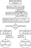Fig. 2. Flowchart of the algorithm followed for the computation of LCS. We note that it requires integration of two dynamical systems. First, the flow of the original dynamical system on a grid must be computed, in order to estimate its Jacobian. After that, we take as initial condition (i.c.) local extrema of the singular values and integrate the field given by the corresponding right-singular vectors.

A strainline or repelling LCS is obtained by taking as initial point x₀ a local maximum of the largest eigenvalue λ₂ and integrating from x₀ the eigenvector field ξ₁ forward and backward in time. Analogously, a stretchline or attracting LCS is obtained by taking as initial point x₀ a local minimum of the smallest eigenvalue λ₁ and integrating from x₀ the eigenvector field ξ₂ forward and backward in time. Let us detail the procedure followed by our software package in order to compute these strain and stretchlines for the flow ${\mathbf{F}}_{t_0}^t$ of a sufficiently smooth dynamical system over a rectangular spatial domain Γ.

Since the eigenvector fields will be determined numerically in a discrete set of points, we define a regular rectangular grid, henceforth called the main grid, covering the domain Γ with steps Δx, Δy along the x, y axes, respectively. For each point x_i = (x, y) in the main grid we compute the Jacobian of the flow ${\mathbf{F}}_{t_0}^t$. When variational equations are available one can easy take the so called state transition matrix resulting from the integration with initial conditions x_i = (x, y). Otherwise one can use the same main grid, or even with smaller steps, to approximate it with a numerical differentiation formula. This is, for each point x_i = (x, y) in the main grid we can select four neighbouring points $x_i^r=(x,y)+({\delta }_x,0),x_i^l=(x,y)-({\delta }_x,0),x_i^u=(x,y)+(0,{\delta }_y),x_i^d=(x,y)-(0,{\delta }_y)$, where δ_x, δ_y define suitable small displacements (see Fig. 3) and then to implement a centred difference scheme,$$\begin{array}{c}\nabla F_{t_0}^t(x_i)\approx \left(\frac{F_{t_0}^t(x_i^r)-F_{t_0}^t(x_i^l)}{2{\delta }_x},\frac{F_{t_0}^t(x_i^u)-F_{t_0}^t(x_i^d)}{2{\delta }_y}\right).\end{array}$$(4)

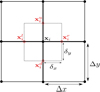Fig. 3. The four neighbouring points (red) to a point xi in the main grid which can be used to compute the Jacobian of the flow $F_{t_0}^t({\text{x}}_i)$ by finite differences.

The accuracy of this computation is crucial and a high order integrator is advisable (we use an adaptive Runge-Kutta-Fehlberg method of order 7–8). Special attention must be paid in the selection of δ_{x, y} when using the numerical differentiation approximation.

Once we have computed the Jacobian of the flow ${\mathbf{F}}_{t_0}^t$ in the points of the main grid, the next step is to perform a singular value decomposition (SVD) on each Jacobian. The purpose of this computation is to obtain the singular values ${\sigma }_1(x_i)=\hspace{0.17em}\left|\right|\nabla F_{t_0}^t\left|\right|\hspace{0.17em}\ge \hspace{0.17em}{\sigma }_2(x_i)$ , and the corresponding right-singular vectors, η₁(x_i), η₂(x_i), for each point of the main grid. We compute directly the SVD of the Jacobian, rather than the diagonalization of the Cauchy-Green tensor, to minimize error transmission from the values of the Jacobian to the result of the computation. In addition, in the cases where the Jacobian is singular, the SVD yields a singular value very close to zero and positive, while the diagonalization of the Cauchy-Green tensor, due to numerical rounding errors, can produce also an eigenvalue very close to zero but it may have positive or negative sign.

When our domain of the phase state, U, has dimension greater than 2, the computation of two-dimensional LCS (strain and stretch lines) can still yield a pretty amount of information about the dynamics of the system by strategically parameterizing selected surfaces S inside the domain U,$$\begin{array}{c}\hfill \begin{array}{cccc}\mathrm{\Psi }:& \mathrm{\Gamma }& ⟶& S\subset U\\ & (\mathrm{\alpha },\mathrm{\beta })& ⟼& \mathbf{x}(\mathrm{\alpha },\mathrm{\beta })\end{array}\end{array}$$(5)

being again Γ a rectangle. The flow ${\tilde{\mathbf{F}}}_{t_0}^t={\mathbf{F}}_{t_0}^t\circ \mathrm{\Psi }$ is now a flow defined on Γ ⊂ R ² to which the above computation can be applied. But in this case special care must be taken to account for the effects of the parametrization Ψ. Now we have $\mathrm{\nabla }{\tilde{\mathbf{F}}}_{t_0}^t=\mathrm{\nabla }{\mathbf{F}}_{t_0}^t·\mathrm{\nabla }\mathrm{\Psi }$, and so the Jacobian ∇Ψ of the parametrization introduces its own compression or spreading of tangent directions, which do not belong to the original flow ${\mathbf{F}}_{t_0}^t$ but it has been artificially inserted by the parametrization Ψ (for instance, the compression towards the north and south poles of a sphere introduced by standard spherical coordinates). The solution to this problem is to apply the SVD to the Jacobian $\nabla F_{t_0}^t$ , expressed in an orthonormal basis w₁, w₂ of the tangent space to the parametrized surface S = Ψ(Γ) at each point x. This depends only on the surface S and the point x, but not on the parametrization Ψ. If C is the base change from this orthonormal basis w₁, w₂ to the original one in our parametrization ∇Ψ(∂_α),∇Ψ(∂_β), then we perform the SVD to the matrix$$\begin{array}{c}\hfill {(\mathrm{\nabla }{\mathbf{F}}_{t_0}^t)}_{|S}(\mathbf{x})=\mathrm{\nabla }{\tilde{\mathbf{F}}}_{t_0}^t(\mathbf{x})·C\end{array}$$(6)

which is the Jacobian of the flow ${\mathbf{F}}_{t_0}^t$ restricted to the surface S using as a departure basis for the tangent space, T_xS, the orthonormal basis w₁, w₂ which does not introduce distortions to the flow.

Finally, according to the above conditions (i)–(iv), the strainlines are computed taking the local maxima of the largest singular value σ₁ in the main grid as initial condition and integrating the right-singular vector field η₂ forward and backward in time. The stretchlines are computed taking the local minima of the smallest singular value σ₂ in the main grid as initial condition, but now integrating the right-singular vector field η₁ forward and backward in time.

Let us note that the vector fields η₁, η₂ to be integrated in the computation of strain and stretch lines are known only in the discrete main grid. Because of this, the use of a variable step integrator requires interpolation of the fields and in fact it does not result in better accuracy for the computed solution. Accordingly, we have selected an order 4 Runge-Kutta (RK4) integrator with a fixed step, taken smaller than the main grid step. Moreover the choice of a fixed step RK4 simple integrator not only speeds up the computations but also handles an added difficulty of the discrete vector fields η₁, η₂. Pointwise, the vectors η₁(x_i), η₂(x_i) are defined up to the sign, which means that the orientation of the field can suddenly reverse. In practice this is indeed the case, since the SVD algorithm produces singular vectors that do not vary continuously, but suddenly change orientation when crossing certain boundaries in the domain. This is unavoidable when the vector field is not parallelizable (see Abraham et al. 1988), which happens for instance when the two singular values σ₁, σ₂ become equal at a point in the domain Γ. We avoid this discontinuity in the sign of the vectors, which would make the integrator to oscillate back and forth, by asking our integrator to compare the orientation of the current vector field value with the previous one used in the integration, and to reverse orientation of the current vector in case that an orientation discontinuity be detected.

Finally, in order to avoid local extreme values of the singular values σ₁, σ₂ introduced by fluctuation errors in their computation, our algorithm fixes a minimal radius such that, only points that are extrema for the singular value within this radius are considered as a starting point for a LCS. Moreover, if one of such points lies within this critical distance of an already computed LCS of its type (strainlines for maxima of the main value σ₁, stretchlines for minima of the smaller value σ₂), then it is discarded as a starting condition of a LCS. The reason for this is that it would produce a line that is superfluous, since it would be closely parallel to an already computed LCS of the same type.

4. LCS in the precessing bar galactic model

The purpose of this paper is the computation of LCS in both the autonomous precessing bar galactic model and a non-autonomous version, and to analise and compare the results with the invariant manifold structure of the same model. Let us start first with a summary of galactic models and the bar precessing one in particular.

Barred galaxies represent about 65% of disc galaxies (Eskridge et al. 2000), characterized mainly by a disc and a central bar-like structure. These components are usually mathematically modelled by analytical potentials (Athanassoula et al. 1983; Pfenniger 1984; Patsis et al. 2003; Skokos et al. 2002, among others). In our work, as in many others, the disc component is described by a Miyamoto-Nagai potential (Miyamoto & Nagai 1975),$$\begin{array}{c}\hfill {\mathrm{\varphi }}_d=-\frac{G{M}_{\mathrm{d}}}{\sqrt{R^2+{(A+\sqrt{B^2+z^2})}^2}},\end{array}$$(7)

where R² = x² + y² is the cylindrical coordinate radius in the disc plane, and z denotes the distance in the out-of-plane component. The parameter G is the gravitational constant and M_d is the mass of the disc while parameters A and B characterize the shape of the disc.

The bar structure is modelled by a Ferrers ellipsoid (Ferrers 1877) with density function,$$\rho =\{\begin{array}{ll}{\rho }_0{(1-m^2)}^{n_{\text{h}}},\hfill & m\le 1,\hfill \\ 0,\hfill & m>1.\hfill \end{array}$$(8)

Here m² = x²/a² + y²/b² + z²/c², and the parameters a (semi-major axis), b (intermediate axis), c (semi-minor axis) determine the shape of the bar while the parameter n_h determines the homogeneity degree for the mass distribution. The parameter ρ₀ is the density at the origin and, thus, the density distribution ρ depends on the degree of homogeneity n_h and the value ρ₀ selected.

The precessing bar galactic model (Sánchez-Martín et al. 2016) is a generalization of the classical galactic model (e.g. Pfenniger 1984; Skokos et al. 2002; Romero-Gómez et al. 2006) formed by a Ferrers bar and a Miyamoto-Nagai disc. In the precessing model the bar is assumed to be tilted and precessing in a small angle ε with respect to the galactic plane (z = 0). So it can be seen as an order ε perturbation of the classical model, which is recovered when ε = 0. A main advantage of the precessing model is that it can explain warp structures that appear in many galaxies.

In a non-inertial reference frame aligned with the main axis of the ellipsoidal bar (see Fig. 4) the equations of motion can be written as the following dynamical system:$$\begin{array}{c}\hfill \{\begin{array}{c}\ddot{x}=2\mathrm{\Omega }cos(\mathrm{\epsilon })\dot{y}+{\mathrm{\Omega }}^2{cos}^2(\mathrm{\epsilon })x+{\mathrm{\Omega }}^{2}sin(\mathrm{\epsilon })cos(\mathrm{\epsilon })z-{\mathrm{\varphi }}_x\hfill \\ \ddot{y}=-2\mathrm{\Omega }cos(\mathrm{\epsilon })\dot{x}-2\mathrm{\Omega }sin(\mathrm{\epsilon })\dot{z}+{\mathrm{\Omega }}^{2}y-{\mathrm{\varphi }}_y\hfill \\ \ddot{z}=2\mathrm{\Omega }sin(\mathrm{\epsilon })\dot{y}+{\mathrm{\Omega }}^{2}sin(\mathrm{\epsilon })cos(\mathrm{\epsilon })x+{\mathrm{\Omega }}^2{sin}^2(\mathrm{\epsilon })z-{\mathrm{\varphi }}_z\hfill \end{array}\end{array}$$(9)

where the constant value Ω is the bar pattern speed and the potential function ϕ is given by the sum of the potentials of the disc and the bar, ϕ = ϕ_d + ϕ_b. We note that when ε = 0 we recover the classical galactic model, and moreover if Ω is set to one, the dynamics of the system is someway similar to the so called Restricted Three Body Problem. The detailed derivation of the equations of motion of the precessing model can be found in Sánchez-Martín et al. (2016).

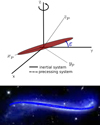Fig. 4. Top: precessing model with major axis of the bar aligned with the precessing x axis, and precessing z axis describing a cone about the inertial Z axis. (xp, yp, zp) denotes the axes in the precessing frame and (X, Y, Z) in the inertial one. Bottom: Integral Sign galaxy, UGC 3697, with a superposition of the warp obtained from the precessing model.

Since our computation of strain and stretch lines is performed on two-dimensional domains, while the phase space of the precessing model is six-dimensional, we select a simplified, yet physically relevant, case of the model whose dynamics can be captured by a well placed parametrized surface inside the phase space (x, y, z, ẋ, ẏ, ż). First, we set the tilt angle ε = 0 (classical model), to model an unwarped ringed galaxy whose dynamics along the z, ż axes are trivial. Next, we fix the values z = 0, ż = 0 to restrict ourselves to the equatorial, or galactic, plane, which is invariant and captures all the dynamics of the galaxy. The dynamics of these two-dimensional galaxy models have been studied in Sánchez-Martín et al. (2016), Romero-Gómez et al. (2006). Let us make a brief summary of their results:

4.1. Dynamics of the precessing model via invariant manifolds

In this paper we consider the parameters, A = 3, B = 1, GM_d = 0.9 for the disc and a = 6, b = 1.5, c = 0.6 for the bar with a pattern speed Ω = 0.05, since these parameters agree with observations and are widely studied (Pfenniger 1984). The dynamics are organized around the five equilibrium points (L_i, i = 1…5) of the model. In the top panel of Fig. 5 we show the equilibrium points and the zero velocity curves of the system. The points L₁, L₂ lie on the x-axis, they are symmetric with respect to the origin, unstable and surrounded by families of periodic orbits. L₄, L₅ lie on the y-axis and are surrounded by families of periodic banana orbits (Athanassoula et al. 1983; Contopoulos 1981; Skokos et al. 2002), while L₃ lies on the origin of coordinates and is linearly stable. The centre panel of Fig. 5 shows the x₁ family of planar periodic orbits about L₃, which is mainly stable and has been regarded as responsible for the skeleton of the bar’s structure. But we are particularly interested in the trajectories outside the bar, driven by the normally hyperbolic invariant manifolds associated to the libration point orbits about L₁ and L₂, since they are responsible of the main visible building blocks in the barred galaxies through the transport of matter. In the bottom panel of Fig. 5 we can observe these invariant manifolds for the set of parameters taken in the paper.

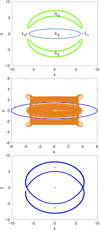Fig. 5. Dynamics in the xy plane of the precessing model with mass bar GMb = 0.1 and tilt angle ε = 0, for which the major axis of the bar rotates counterclockwise inside this plane. Top: Lagrange points and zero velocity curves for Jacobi constant CJ = −0.1876 (Ferrers bar of the model is outlined by the blue curve). Centre: in orange lines, family of periodic orbits of the mode, Ferrers bar in blue. Bottom: in blue, unstable invariant manifolds. In red, Lagrange points of the system.

Thus, the stable and unstable manifolds of periodic orbits of the same energy level (from now on denoted by $W_{{\gamma }_i}^s\hspace{0.17em}\text{and}\hspace{0.17em}{W}_{{\gamma }_j}^u$, where γ_i,γ_j indicate the periodic orbit), as well as their intersections, give rise to the responsible structures for the transport of matter in the galaxy. In this context, we call heteroclinic orbits the orbits which correspond to asymptotic trajectories, ψ, such that $\psi \in W_{{\gamma }_i}^u{{\displaystyle \cap }}^{\text{}}{W}_{{\gamma }_j}^s,\hspace{0.17em}i\ne j,i,\hspace{0.17em}j=1,2$ , while homoclinic orbits correspond to the asymptotic trajectories ψ when i = j.

The formation of pseudo-rings, rings and spirals in barred galaxies is related, besides to the invariant manifolds, to the existence of heteroclinic and homoclinic orbits. Following the classical nomenclature of inner rings (r) and outer rings (R), outer rings are called, R₁ when they have the major axis perpendicular to the bar major axis, R₂ if they have the major axis along the bar major axis and, R₁R₂ when they have a component parallel and another one perpendicular to the bar. As explained in Romero-Gómez et al. (2006, 2007), the formation of rR₁ rings is linked to the existence of heteroclinic orbits, R₁R₂ is linked to the existence of homoclinic ones, while spiral arms and R₂ rings appear when there exist neither heteroclinic nor homoclinic orbits.

So for instance, the existence of these heteroclinic orbits makes the galaxy a rR₁ ringed galaxy, because they establish a closed path along which the matter is transported (Fig. 6). The transfer of matter happens mainly from the inner region delimited between the bar and the zero velocity curves to the outer region. The transit orbits contained inside the manifold tubes (Romero-Gómez et al. 2006, 2007; Gidea & Masdemont 2007) are responsible for this action. On the other hand, the non-transit orbits are those that stay out of the manifold tube and move only around the bar without going out to the outer regions.

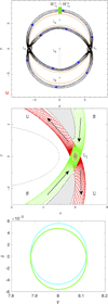Fig. 6. Dynamics of a rR1 ringed galaxy. Top: in blue, arrows indicating circulation of matter. In green, intersection of the invariant manifolds with hyperplane S. All of them in the (x, y) plane (image adapted from Athanassoula et al. 2009). Centre: neighbourhood of equilibrium point L1 in (x, y) plane. Arrows: motion along invariant manifolds (S = stable, U = unstable). Stripped areas: forbidden regions delimited by zero velocity curves (image taken from Athanassoula et al. 2009). Bottom: precessing model with masses GMb = 0.1, GMd = 0.9, pattern speed Ω = 0.05, and tilt angle ε = 0. We display the (y, ẏ) projections of the first crossings of the unstable and stable manifolds with the hyperplane S. In cyan: $W_{{\gamma }_1}^{s,1}$, in green: $W_{{\gamma }_2}^{u,1}$. See more details in the text.

As the dynamics of our system takes place in a six dimensional phase space, we compute the intersections of the trajectories of the invariant manifolds with the hyperplane S given by the section x = 0 in phase space. We consider the outer branches of the stable invariant manifold of the Lyapunov orbit around L₁, $W_{{\gamma }_1}^s$ , and the unstable invariant manifold of the Lyapunov orbit around L₂, $W_{{\gamma }_2}^u$ , both at the same energy level. The first intersection of these two invariant manifolds with the hyperplane S are two closed curves. Considering the y ẏ projection, we denote by $W_{{\gamma }_1}^{s,1}$ the closed curve resulting from the first intersection of $W_{{\gamma }_1}^s$ , and by $W_{{\gamma }_2}^{u,1}$ the closed curve resulting from the first intersection of $W_{{\gamma }_2}^u$ . The intersection $W_{{\gamma }_1}^{s,1}\cap W_{{\gamma }_2}^{u,1}$ corresponds to heteroclinic orbits for the given energy level of the invariant manifolds. Analogously, the second intersection of the invariant manifolds $W_{{\gamma }_1}^s,\hspace{0.17em}{W}_{{\gamma }_2}^u$ with the hyperplane S are denoted by $W_{{\gamma }_1}^{s,2}\hspace{0.17em}\text{and}\hspace{0.17em}{W}_{{\gamma }_2}^{u,2}$ respectively.

When the tilt angle ε takes the value ε = 0, the plane z = 0 is invariant, so the phase space is reduced to four dimensions, which, together with the fixed energy level let us define a state just selecting a (y, ẏ) point on S (this is, a point on S is defined by x = 0, and since z = ż = 0, selecting y and ẏ, for the fixed energy level and the sense of crossing, also ẋ is determined, completing this way the state).

Then the points on the curve $W_{{\gamma }_1}^{s,1}$ correspond to states on $W_{{\gamma }_1}^s$ and so they are orbits that tend asymptotically to the Lyapunov orbit γ₁. In the same way, the points on the curve $W_{{\gamma }_2}^{u,1}$ provide states on $W_{{\gamma }_2}^u$, therefore they are orbits that depart asymptotically from the Lyapunov orbit γ₂. This means that when γ₁ and γ₂ are both in the same energy level, the intersection points $W_{{\gamma }_1}^{s,1}\cap W_{{\gamma }_2}^{u,1}$ correspond to heteroclinic orbits between them. In the bottom panel of Fig. 6 we observe that for ε = 0 there are two heteroclinic orbits corresponding to the intersection of $W_{{\gamma }_1}^{s,1}\hspace{0.17em}\text{and}\hspace{0.17em}{W}_{{\gamma }_2}^{u,1}$.

As it is known, the (y, ẏ) points outside both curves, $W_{{\gamma }_1}^{s,1}\hspace{0.17em}\text{and}\hspace{0.17em}{W}_{{\gamma }_2}^{u,1}$, correspond to states whose trajectories remain inside the inner region of the galaxy delimited by the zero velocity curves, meaning they are non-transit orbits. Finally the (y, ẏ) points that are inside the intersection defined by both curves correspond to orbits that transit from the inner region to the outer one, meaning they are transit orbits. It is in this way how the invariant manifolds of the Lyapunov orbits drive the motion of the stars from the inner to the outer regions. See Fig. 6 and also Sánchez-Martín (2015) for many more details.

4.2. Dynamics of the precessing model via LCS

In order to obtain a surface containing the heteroclinic orbits between the L₁ and L₂ regions of our model, we fix an energy level C_L1 + δ slightly above of that of the equilibrium point L₁ (or L₂) and we set x = 0. As we have already mentioned, the states of the system on this surface can be parameterised by (y, ẏ) since using the Jacobi constant of the system,$$\begin{array}{cc}\hfill C(x,y,z,\dot{x},\dot{y},\dot{z})=& -({\dot{x}}^2+{\dot{y}}^2+{\dot{z}}^2)+2{\mathrm{\Omega }}^{2}sin(\mathrm{\epsilon })cos(\mathrm{\epsilon })xz\hfill \\ \hfill & +{\mathrm{\Omega }}^2({cos}^2(\mathrm{\epsilon })x^2+y^2+{sin}^2(\mathrm{\epsilon })z^2)-2\mathrm{\varphi },\hfill \end{array}$$(10)

and taking into account that for planar orbits z = ż = 0, we obtain ẋ as,$$\begin{array}{c}\hfill \dot{x}=\sqrt{-{\dot{y}}^2+{\mathrm{\Omega }}^2{y}^2-2\mathrm{\varphi }(0,y,0)-(C_{L_1}+\delta )}.\end{array}$$(11)

In this way we have a surface S ⊂ ℝ⁶ parametrised by$$\begin{array}{c}\hfill \mathrm{\Psi }(y,\dot{y})=(0,y,0,\sqrt{-{\dot{y}}^2+{\mathrm{\Omega }}^2{y}^2-2\mathrm{\varphi }(0,y,0)-(C_{L_1}+\delta )},\dot{y},0),\end{array}$$(12)

where we have chosen the positive value of ẋ, to obtain the plane containing the above mentioned heteroclinic orbits (from the L₂ neighbourhood to the L₁ one, this is, we cross S from x < 0 to x > 0).

We consider the same parameters as in the previous case. Unless otherwise indicated, the spatial domain for our parametrization is Γ = [7.8, 8.2]×[−0.007, 0.007]. Figure 7 shows the FTLE field and the strainlines corresponding to this model for an integration time T = [0, 505], where t = 505 is the time of the first intersection of the upper branch of the stable invariant manifold with the x = 0 plane. We note that the concentration of strainlines is found on the main ridges of the FTLE field, forming a closed curve.

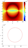Fig. 7. FTLE (top) and strainlines (bottom) of the classical model for time T = [0, 505].

Let us overimpose the FTLE field, the strainlines and the first cuts of the heteroclinic orbits with the {x = 0, y ≥ 0} semiplane, for the same level of energy (C_L1 + δ, with δ small). Figure 8 shows in the top panel how the strainlines follow the main ridge of the FTLE field. If we observe $W_{{\gamma }_1}^{s,1}\hspace{0.17em}\text{and}\hspace{0.17em}{W}_{{\gamma }_2}^{u,1}$ (centre panel), the one corresponding to the stable manifold follows as well the main ridge of the FTLE field, whereas the one corresponding to the unstable manifold is associated with the boundary of the ridge. When we join both figures, in the bottom panel, the strainlines correspond exactly with the heteroclinic orbit of the stable manifold. Therefore, we confirm that the strainlines are associated with the stable invariant manifolds, and more precisely with $W_{{\gamma }_1}^{s,1}$, at least in the autonomous problem. Let us remark that as the stretchlines are by definition perpendicular to the strainlines, they do not seem to carry any relevant dynamic information in our problem.

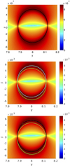Fig. 8. Classical model for time T = [0, 505]. Top: FTLE field and strainlines in black. Centre: FTLE field and heteroclinic orbits ($W_{{\gamma }_1}^{s,1}$ in cyan, $W_{{\gamma }_2}^{u,1}$ in green). Bottom: FTLE field, strainlines (in black) and heteroclinic orbits (in cyan and green). Cyan and black coincide perfectly.

When the integration time is increased, the accuracy of the description of the FTLE field and strainlines is gradually lost. This is due not only to the loss of accuracy in the integration of the dynamical system when computing the LCS, but also to the fact that, in the classical model, the successive intersections of the invariant manifolds with the semiplane {x = 0, y ≥ 0} become increasingly blurred due to the transversal intersection of manifolds and the inherent chaotic dynamics (see Gidea & Masdemont 2007). Taking an integration time T = [0, 1000] the ridges of the FTLE field are not so remarked, but the strainlines continue following these ridges, although the dynamics of the system is less clear (see Fig. 9).

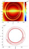Fig. 9. FTLE (top) and strainlines (bottom) of the classical model for time T = [0, 1000].

In order to observe the second intersection of the invariant manifolds with the semiplane {x = 0, y ≥ 0}, $W_{{\gamma }_1}^{s,2}\hspace{0.17em}\text{and}\hspace{0.17em}{W}_{{\gamma }_2}^{u,2}$, and the corresponding LCS, we take a time interval for the integration of T = [0, 1570]. Figure 10 shows the FTLE field, where the ridges are less marked than in the previous case, as well as the strainlines associated with these ridges, but still the impact of the chaotic dynamics is noticed with some structure. However we also observe some artifacts in the integration of strainlines that do not correspond to ridges of the FTLE field, but are due to the long time of integration, for example in the top right part of the figure of strainlines.

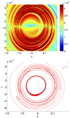Fig. 10. FTLE (top) and strainlines (bottom) of the classical model for time T = [0, 1570].

In Fig. 11 we observe how the strainlines (in black) follow the main ridges of the FTLE field, although some of the strainlines do not match these ridges (top panel). In the centre panel we show the cuts of the heteroclinic orbits, $W_{{\gamma }_1}^{s,2}\hspace{0.17em}\text{and}\hspace{0.17em}{W}_{{\gamma }_2}^{u,2}$, superimposed to the FTLE field, where we mark this second intersection of the invariant manifolds with dots in order to clarify the figure, since they do not follow a clear closed curve. We observe that the second intersection of the stable manifold (in blue) follows approximately the ridges of the FTLE field. To join this stable manifold to the strainlines and the FTLE field (bottom panel), the stable manifold (the first intersection with the plane x = 0 in magenta, the second one in blue) is closely approximated by the strainlines and the ridges of the FTLE field in its main components. Let us point out that both the strainlines and the ridges of the FTLE field also give false positives as time increases, that is, not all the strainlines follow the ridges of the FTLE field and furthermore some ridges of the FTLE field do not correspond to a defined structure of the dynamics of the model. This fact suggests that for long integration times the FTLE field and the strainlines lose its precision, a fact that is also stated by Farazmand & Haller (2012).

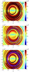Fig. 11. Classical model for time T = [0, 1570]. Top: FTLE field and strainlines in black. Centre: FTLE field and heteroclinic orbits for the second intersection of the {x = 0, y ≥ 0} semiplane ($W_{{\gamma }_1}^{s,2}$ in blue, $W_{{\gamma }_2}^{u,2}$ in green). Bottom: FTLE field, strainlines (in black) and heteroclinic orbits for the first intersection (in magenta), $W_{{\gamma }_1}^{s,1}$, and for the second one (in blue), $W_{{\gamma }_1}^{s,2}$, of the stable manifold.

For the integration time of T = [0, 505], for which we obtain good accuracy, we now increase the spatial domain Γ to [7, 9.5]×[−0.1, 0.1] (Fig. 12). The left part of both plots, in dark blue in the FTLE field, shows the region of forbidden motion, where the black dots indicate starting points in the computation of LCS. In the FTLE field as well as in the strainlines, we observe structures within the fixed energy level reflecting the dynamics of the system, corresponding to the heteroclinic orbits and probably to further features, such as intersections of the parametrised surface with other invariant manifolds.

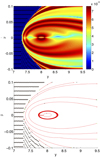Fig. 12. FTLE (top) and strainlines (bottom) of the classical model for time T = [0, 505] in the spatial domain [7, 9.5]×[−0.1, 0.1].

Figure 13 represents the superposition of the FTLE field and the strainlines (top panel), the FTLE field and the heteroclinic orbits (centre panel) and the three elements in the bottom panel. The heteroclinic orbits correspond to the central closed curve, whereas the rest of the main ridges of the FTLE field are followed by the strainlines. This suggests that there are stable manifolds with the same level of energy associated to other structures, which are easily captured by the main ridges of the FTLE field and the corresponding strainlines.

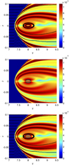Fig. 13. Classical model for time T = [0, 505] in the spatial domain [7, 9.5]×[−0.1, 0.1]. Top: FTLE field and strainlines in black. Centre: FTLE field and heteroclinic orbits ($W_{{\gamma }_1}^{s,1}$ in blue, $W_{{\gamma }_2}^{u,1}$ in green). Bottom: FTLE field, strainlines (in black) and heteroclinic orbits (in blue and green).

4.3. LCS in the non-autonomous case

In the autonomous problem we observed that the FTLE field and its corresponding strainlines are good indicators, analogue to the stable invariant manifolds. However the main purpose of LCS is to study the dynamics of non-autonomous problems where the computation of invariant manifolds is much more complex or when the basic structure associated to the invariant manifold (e.g. equilibrium point or periodic orbit) does not exist and so, the invariant manifolds are not defined. For these cases the computation of LCS still remains simple and valid, describing pretty well the organization of the motion moreover they can be seen as an extension of the invariant manifolds for the autonomous problems. With this idea we transform our precessing model into a non-autonomous model to observe the behaviour of its dynamics.

According to Widrow et al. (2008); Manos & Machado (2014) (among others) a parameter which is dependent on time in galaxy models is its pattern speed. The decrease in the pattern speed over time has been observed in galaxies, due to the transfer of angular momentum from the bar to the other components of the galaxy. So in this section, we consider a pattern speed depending on time in the precessing model, ${\tilde{\mathrm{\Omega }}}_{\mathbf{p}}={\mathrm{\Omega }}_{\mathbf{p}}(t)$, and this dependence introduces changes to the equations of the model. The vectorial form of the equations of motion in the rotating reference frame is now,$$\begin{array}{c}\hfill \ddot{\mathbf{r}}=-\mathrm{\nabla }\mathrm{\varphi }-2({\tilde{\mathrm{\Omega }}}_{\mathbf{p}}\times \dot{\mathbf{r}})-{\tilde{\mathrm{\Omega }}}_{\mathbf{p}}\times ({\tilde{\mathrm{\Omega }}}_{\mathbf{p}}\times \mathbf{r})-{\dot{\tilde{\mathrm{\Omega }}}}_{\mathbf{p}}\times \mathbf{r},\end{array}$$(13)

where the term $-{\dot{\tilde{\mathrm{\Omega }}}}_{\mathbf{p}}\times \mathbf{r}$ is the inertial force of rotation (see Binney & Tremaine 2008, for further details).

Taking ${\tilde{\mathrm{\Omega }}}_{\mathbf{p}}$ as in Sánchez-Martín et al. (2016), but now with $\tilde{\mathrm{\Omega }}=\tilde{\mathrm{\Omega }}(t)$ depending on time,$$\begin{array}{c}\hfill {\tilde{\mathrm{\Omega }}}_{\mathbf{p}}=(-\tilde{\mathrm{\Omega }}sin(\mathrm{\epsilon }),0,\tilde{\mathrm{\Omega }}cos(\mathrm{\epsilon })),\end{array}$$(14)

the new equations of motion are given by$$\begin{array}{c}\hfill \{\begin{array}{c}\ddot{x}=2\tilde{\mathrm{\Omega }}cos(\mathrm{\epsilon })\dot{y}+{\tilde{\mathrm{\Omega }}}^2{cos}^2(\mathrm{\epsilon })x+{\tilde{\mathrm{\Omega }}}^{2}sin(\mathrm{\epsilon })cos(\mathrm{\epsilon })z+\dot{\tilde{\mathrm{\Omega }}}cos(\mathrm{\epsilon })y-{\mathrm{\varphi }}_x\hfill \\ \ddot{y}=-2\tilde{\mathrm{\Omega }}cos(\mathrm{\epsilon })\dot{x}-2\tilde{\mathrm{\Omega }}sin(\mathrm{\epsilon })\dot{z}+{\tilde{\mathrm{\Omega }}}^{2}y-\dot{\tilde{\mathrm{\Omega }}}cos(\mathrm{\epsilon })x-\dot{\tilde{\mathrm{\Omega }}}sin(\mathrm{\epsilon })z-{\mathrm{\varphi }}_y\hfill \\ \ddot{z}=2\tilde{\mathrm{\Omega }}sin(\mathrm{\epsilon })\dot{y}+{\tilde{\mathrm{\Omega }}}^{2}sin(\mathrm{\epsilon })cos(\mathrm{\epsilon })x+{\tilde{\mathrm{\Omega }}}^2{sin}^2(\mathrm{\epsilon })z+\dot{\tilde{\mathrm{\Omega }}}sin(\mathrm{\epsilon })y-{\mathrm{\varphi }}_z.\hfill \end{array}\end{array}$$(15)

Let us remark that this system is non-autonomous, it has no integrals of motion, and in particular it does not preserve energy, so there are no constant-energy surfaces as in the autonomous precessing model. However in order to parametrise a surface to compute the FTLE field and the strainlines, we can consider the same conditions as in the previous case, taking the Jacobi constant function of the autonomous problem, Eq. (10) with $\mathrm{\Omega }=\tilde{\mathrm{\Omega }}$.

The parameters taken for the bar and disc are the same as previously, but now the pattern speed varies linearly from ${\tilde{\mathrm{\Omega }}}_{t_0}=0.05$ to ${\tilde{\mathrm{\Omega }}}_{t_f}=0.04$ for [t₀, t_f]=[0, 1500] time units, that is, with slope $\dot{\tilde{\mathrm{\Omega }}}=-\frac{2}{3}\times {10}^{-5}$. In the autonomous case, variations of pattern speed for Ω = 0.05 (shown in bottom panel of Fig. 5) to Ω = 0.04 (shown in Fig. 14) causes an increase of the period and the radius of the point L₁ by a factor of 1.2. The effect in the galaxy is to open the internal ring.

The decreasing slope of the pattern speed over time is in agreement to the behaviour observed in N-body simulations, due to the transfer of angular momentum from the bar to the other components of the galaxy (e.g. Widrow et al. 2008) In addition, the starting “energy” level continues to be C_L1 + δ, where C_L1 is the Jacobi constant for the equilibrium point L₁ in the autonomous problem. The selected spatial domain for the integration is Γ = [7.5, 8.7] × [−0.02, 0.02].

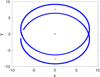Fig. 14. Unstable invariant manifolds (blue) and Lagrange points (red) of the model with mass bar GMb = 0.1, tilt angle ε = 0 and Ω = 0.04 in the xy plane.

In order to compare the new results with the ones obtained for the autonomous classical model, we take the same integration times. The first computation of LCS is for the time interval T = [0, 505] (Fig. 15). We observe that although the problem is non-autonomous, the shape of the main ridges of the FTLE field and the strainlines continues being that of a closed curve, and that the strainlines still follow the main ridges of the FTLE field. But, if we superimpose the cuts $W_{{\gamma }_1}^{s,1}\hspace{0.17em}\text{and}\hspace{0.17em}{W}_{{\gamma }_2}^{u,1}$ of the invariant manifolds of the autonomous model, we observe that the widths of the FTLE field and strainlines have increased (Fig. 16). Since the integration time is the same as the one taken in the autonomous problem (Fig. 8), the different range in the spatial domain is due to a variation of energy when integrating the initial conditions. This variation takes place because the function chosen to parametrise the surface of initial conditions is not an integral of motion of the non-autonomous model, and therefore the “energy” of the system given by this function in fact changes, as we observe in the bottom right panel of Fig. 16. Let us point out that in this figure the strainlines are associated with an abrupt change of energy.

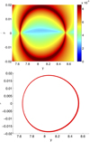Fig. 15. FTLE (top) and strainlines (bottom) of the non-autonomous classical model with tilt angle ε = 0 for time T = [0, 505].

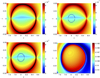Fig. 16. Non-autonomous classical model for time T = [0, 505]. Top left: FTLE field and strainlines in black. Top right: FTLE field and heteroclinic orbits of the autonomous classical model ($W_{{\gamma }_1}^{s,1}$ in blue, $W_{{\gamma }_2}^{u,1}$ in green). Bottom left: FTLE field, strainlines (in black) and heteroclinic orbits of the autonomous classical model (in blue and green). Bottom right: energy at the endpoint of each orbit.

Figure 17 displays the FTLE field and the strainlines for an integration time of T = [0, 1000], and the same spatial domain as in the previous integration for time T = [0, 505] of the non-autonomous problem. While in the integration of the autonomous classical model both FTLE ridges and strainlines became blurred and separated from heteroclinic orbits when the integration time increased to 1000, here they suffer a much smaller deformation compared to their position for integration time T = [0, 505].

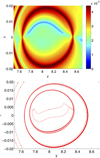Fig. 17. FTLE (top) and strainlines (bottom) of the non-autonomous classical model for time T = [0, 1000].

Figure 18 presents the strainlines overimposed on the FTLE field (top panel) and the final value of the energy in each orbit (bottom panel). Comparing the results with those of integration time T = [0, 505], we notice that an FTLE ridge-cum-strainline appears for values of y up to 7.7. The main strainlines follow the ridges of the FTLE field, but there is a secondary ring of central strainlines inside the main FTLE ridge that does not correspond to any feature of the FTLE field. In the bottom panel we observe that the main strainlines coincide with an abrupt variation of the final energy level of each orbit, and the central strainlines are placed over a smoother variation of the final energy level. An isolated central strainline diverging from the inner ring seems an artifact introduced by inaccuracies accumulated over the long integration time.

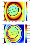Fig. 18. Non-autonomous classical model for time T = [0, 1000]. Top: FTLE field and strainlines in black. Bottom: energy at the endpoint of each orbit.

Figure 19 shows the FTLE field and the strainlines for an interval of integration of T = [0, 1570]. The distribution of values of the FTLE field is very similar to that of the interval of integration T = [0, 1000]. Regarding the strainlines, they cover the ridges of the FTLE field and there is a further inner ring of strainlines inside the main ridge of the FTLE field following a lesser ridge that borders areas of decrease of the FTLE field.

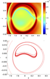Fig. 19. FTLE (top) and strainlines (bottom) of the non-autonomous precessing model with tilt angle ε = 0 for time T = [0, 1570].

Figure 20 illustrates that the behaviour of the strainlines in relation to the final energy of the orbits for integration time T = [0, 1570] is the same as for integration time T = [0, 1000]. Therefore, the main rings of strainlines border on the steepest variations of energy level and the inner ring of strainlines also borders on a secondary area of variation of the energy level.

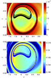Fig. 20. Non-autonomous precessing model with tilt angle ε = 0 for time T = [0, 1570]. Top: FTLE field and strainlines in black. Bottom: energy at the endpoint of each orbit.

Finally Fig. 21 shows the strainlines, FTLE field and final energy level for the orbits for a wider parametrised surface in the spatial domain $(y,\dot{y})\in \mathrm{\Gamma }=[7,9.5]\times [-0.1,0.1]$, for integration times T = [0, 505] in the left column and T = [0, 1000] in the right column. Looking at the FTLE field and the strainlines (top row) we see that there are more ridges of the FTLE field and strainlines surrounding the main one seen on the previous figures. A longer integration time leads to the appearance of further features (FTLE ridges and strainlines) of this type. The comparison of the final energy level of the orbits with the strainlines (bottom row) establishes that the strainlines point out curves of steepest variation for the final energy level of the orbits.

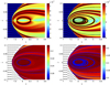Fig. 21. Non-autonomous precessing model with tilt angle ε = 0 for time T = [0, 505] and T = [0, 1000]. Top: FTLE field and strainlines in black for time T = [0, 505] (left) and T = [0, 1000] (right). Bottom: energy at the endpoint of each orbit for time T = [0, 505] (left) and T = [0, 1000] (right), and strainlines (in blue).

To sum up the computations of this section, we can state that FTLE ridges are covered by strainlines, that there appear some further strainlines associated to secondary features of the FTLE field (typically abrupt descents of the field value) and that strainlines in both cases mark curves of steepest descents of the final energy level of the orbits.

Our computations also show that the non-autonomous precessing model presents more stable FTLE field and strainlines than the autonomous version. This greater stability might be due to the energy-dissipative character of our non-autonomous model.

5. Discussion and conclusions

One of the main concerns when applying the manifold theory to barred galactic models is to know how it behaves when the system is under a certain secular evolution. The main goal of this paper is to establish the behaviour of our model in its non-autonomous version, in particular we want to assess whether an adiabatic decrease of the bar pattern speed can change the global morphology of the galaxy, as predicted by the invariant manifolds in the autonomous model. Since invariant manifolds do not exist as such in the non-autonomous problem, we introduce the LCS, and therefore, this paper deals with the study of the non-autonomous version of the galactic model in two dimensions by means of LCS. This is a recently developed theory to determine dynamical structures, either attracting or repelling, reflecting the dynamics of the system in non-autonomous problems. To apply this theory to our galactic model, we have created our own LCS computation software, made as accurate and efficient as possible, and capable of computing LCS in general two-dimensional dynamical systems and in parametrized surfaces in dynamical systems of any dimension. The LCS are based on the singular values and vectors of the Jacobian of the flow, equivalent to the eigenvalues and the eigenvectors of the Cauchy-Green tensor. In particular, the FTLE field is determined by the main singular value, i.e. the norm, of the Jacobian of the flow. Roughly speaking, these LCS give us the repulsion and attraction zones. In two-dimensional domains, we obtain strainlines and stretchlines which are the maximally repelling or attracting lines, respectively. Whereas for the strainlines we have found that they give us relevant information about the dynamics of the system, the strecthlines have turned out to be more ill-conditioned and less connected to the global dynamics of the system. Let us also remark that the LCS must be applied to “smooth problems”, in the sense that the problems have no abrupt changes in its behaviour, since the computation of the flow Jacobian and, above all, of the stretchlines, is very sensitive to sudden variations of the integrated vector field.

In order to better understand the information given by the FTLE field and the LCS, we apply it first to the autonomous galactic model. By selecting a parametrized surface given by the energy of the system in one of the equilibrium points (L₁ or L₂), and initial conditions in the $(y,\dot{y})$ plane, we obtain that the flow Jacobian norm field points to the zones where the stable invariant manifold is placed, and the strainlines accurately overlap with this stable manifold. As the integration time increases, the unavoidable build up of error in the computation of the flow causes it to lose precision in the related flow Jacobian norm field and therefore in the strainline computations, but these still approximate the related stable manifolds. Moreover, the flow Jacobian norm field and the LCS give information about other zones of maximal repulsion placed in a bigger spatial domain, which seem to correspond to invariant manifolds caused by other structures.

We then apply the LCS to the non-autonomous problem, although the energy is not preserved anymore. Selecting the same time intervals of integration as previously, we observe that the flow Jacobian norm field and the strainlines continue remarking the zones of maximal repulsion, with a shape analogous to the previous stable invariant manifold, but with a greater width. In contrast with the autonomous case, in this non-autonomous galactic model the flow Jacobian norm field and the strainlines are not distorted as the integration time increases. This stronger stability seems to be a consequence of the energy-dissipative character of the selected model. In addition, the other zones of maximal repulsion found in the autonomous problem continue existing in this time-dependent model, but now we observe that these zones are placed where a steepest change on the energy of the system happens.

From this study we can derive two main conclusions. First, the LCS strainlines of the non-autonomous galactic problem indicate zones of maximal repulsion in the domain and they are related to the stable manifolds of the galactic autonomous problem when this problem is integrated forward in time, or to its unstable manifolds when it is integrated backwards in time. Second, for a fixed set of input parameters defining the autonomous galactic problem, the invariant manifolds drive the motion of stars through the unstable periodic orbits giving the galaxy a certain morphology, namely ringed or spiral barred galaxy. When allowing a certain adiabatic secular evolution to the system, in this case, in the form of a slow decrease of the bar pattern speed with time, as seen from N-body simulations Widrow et al. (2008), e.g.), the invariant manifolds prediction still holds, since the LCS and the strainlines generalize the dynamics predicted by the manifolds.

Acknowledgments

This work started as part of the doctoral dissertation of P.S.M., supported by the Catalan PhD grants FI-AGAUR and FPU-UPC. J.J.M. thanks MINECO-FEDER (Spanish Ministry of Economy) for the grant MTM2015-65715-P, and the Catalan government for the grant 2017SGR1049. M.R.G. thanks MINECO for the grant ESP2016-80079-C2-1-R (MINECO/FEDER, UE) and MDM-2014-0369 of ICCUB (Unidad de Excelencia “María de Maeztu”).

References

All Figures

Fig. 1. Neighbourhood of a hyperbolic equilibrium point in a two-dimensional, autonomous, dynamical system: The blue segment of initial conditions from Q0 to R0, transverse to the stable invariant manifold, will undergo great stretch when the system is integrated from time t0 to tf and it transforms into the curve from Qf to Rf. Conversely, the red segment of initial conditions from Q0 to S0 will undergo great compression when the system is integrated and it transforms into the curve from Qf to Sf. Any segment of initial conditions not intersecting the invariant manifolds will undergo lesser stretches or strains.

In the text

Fig. 2. Flowchart of the algorithm followed for the computation of LCS. We note that it requires integration of two dynamical systems. First, the flow of the original dynamical system on a grid must be computed, in order to estimate its Jacobian. After that, we take as initial condition (i.c.) local extrema of the singular values and integrate the field given by the corresponding right-singular vectors.

In the text

	Fig. 3. The four neighbouring points (red) to a point xi in the main grid which can be used to compute the Jacobian of the flow $F_{t_0}^t({\text{x}}_i)$ by finite differences.
In the text

	Fig. 4. Top: precessing model with major axis of the bar aligned with the precessing x axis, and precessing z axis describing a cone about the inertial Z axis. (xp, yp, zp) denotes the axes in the precessing frame and (X, Y, Z) in the inertial one. Bottom: Integral Sign galaxy, UGC 3697, with a superposition of the warp obtained from the precessing model.
In the text

Fig. 5. Dynamics in the xy plane of the precessing model with mass bar GMb = 0.1 and tilt angle ε = 0, for which the major axis of the bar rotates counterclockwise inside this plane. Top: Lagrange points and zero velocity curves for Jacobi constant CJ = −0.1876 (Ferrers bar of the model is outlined by the blue curve). Centre: in orange lines, family of periodic orbits of the mode, Ferrers bar in blue. Bottom: in blue, unstable invariant manifolds. In red, Lagrange points of the system.

In the text

Fig. 6. Dynamics of a rR1 ringed galaxy. Top: in blue, arrows indicating circulation of matter. In green, intersection of the invariant manifolds with hyperplane S. All of them in the (x, y) plane (image adapted from Athanassoula et al. 2009). Centre: neighbourhood of equilibrium point L1 in (x, y) plane. Arrows: motion along invariant manifolds (S = stable, U = unstable). Stripped areas: forbidden regions delimited by zero velocity curves (image taken from Athanassoula et al. 2009). Bottom: precessing model with masses GMb = 0.1, GMd = 0.9, pattern speed Ω = 0.05, and tilt angle ε = 0. We display the (y, ẏ) projections of the first crossings of the unstable and stable manifolds with the hyperplane S. In cyan: $W_{{\gamma }_1}^{s,1}$, in green: $W_{{\gamma }_2}^{u,1}$. See more details in the text.

In the text

	Fig. 7. FTLE (top) and strainlines (bottom) of the classical model for time T = [0, 505].
In the text

	Fig. 8. Classical model for time T = [0, 505]. Top: FTLE field and strainlines in black. Centre: FTLE field and heteroclinic orbits ($W_{{\gamma }_1}^{s,1}$ in cyan, $W_{{\gamma }_2}^{u,1}$ in green). Bottom: FTLE field, strainlines (in black) and heteroclinic orbits (in cyan and green). Cyan and black coincide perfectly.
In the text

	Fig. 9. FTLE (top) and strainlines (bottom) of the classical model for time T = [0, 1000].
In the text

	Fig. 10. FTLE (top) and strainlines (bottom) of the classical model for time T = [0, 1570].
In the text

Fig. 11. Classical model for time T = [0, 1570]. Top: FTLE field and strainlines in black. Centre: FTLE field and heteroclinic orbits for the second intersection of the {x = 0, y ≥ 0} semiplane ($W_{{\gamma }_1}^{s,2}$ in blue, $W_{{\gamma }_2}^{u,2}$ in green). Bottom: FTLE field, strainlines (in black) and heteroclinic orbits for the first intersection (in magenta), $W_{{\gamma }_1}^{s,1}$, and for the second one (in blue), $W_{{\gamma }_1}^{s,2}$, of the stable manifold.

In the text

	Fig. 12. FTLE (top) and strainlines (bottom) of the classical model for time T = [0, 505] in the spatial domain [7, 9.5]×[−0.1, 0.1].
In the text

	Fig. 13. Classical model for time T = [0, 505] in the spatial domain [7, 9.5]×[−0.1, 0.1]. Top: FTLE field and strainlines in black. Centre: FTLE field and heteroclinic orbits ($W_{{\gamma }_1}^{s,1}$ in blue, $W_{{\gamma }_2}^{u,1}$ in green). Bottom: FTLE field, strainlines (in black) and heteroclinic orbits (in blue and green).
In the text

	Fig. 14. Unstable invariant manifolds (blue) and Lagrange points (red) of the model with mass bar GMb = 0.1, tilt angle ε = 0 and Ω = 0.04 in the xy plane.
In the text

	Fig. 15. FTLE (top) and strainlines (bottom) of the non-autonomous classical model with tilt angle ε = 0 for time T = [0, 505].
In the text

Fig. 16. Non-autonomous classical model for time T = [0, 505]. Top left: FTLE field and strainlines in black. Top right: FTLE field and heteroclinic orbits of the autonomous classical model ($W_{{\gamma }_1}^{s,1}$ in blue, $W_{{\gamma }_2}^{u,1}$ in green). Bottom left: FTLE field, strainlines (in black) and heteroclinic orbits of the autonomous classical model (in blue and green). Bottom right: energy at the endpoint of each orbit.

In the text

	Fig. 17. FTLE (top) and strainlines (bottom) of the non-autonomous classical model for time T = [0, 1000].
In the text

	Fig. 18. Non-autonomous classical model for time T = [0, 1000]. Top: FTLE field and strainlines in black. Bottom: energy at the endpoint of each orbit.
In the text

	Fig. 19. FTLE (top) and strainlines (bottom) of the non-autonomous precessing model with tilt angle ε = 0 for time T = [0, 1570].
In the text

	Fig. 20. Non-autonomous precessing model with tilt angle ε = 0 for time T = [0, 1570]. Top: FTLE field and strainlines in black. Bottom: energy at the endpoint of each orbit.
In the text

	Fig. 21. Non-autonomous precessing model with tilt angle ε = 0 for time T = [0, 505] and T = [0, 1000]. Top: FTLE field and strainlines in black for time T = [0, 505] (left) and T = [0, 1000] (right). Bottom: energy at the endpoint of each orbit for time T = [0, 505] (left) and T = [0, 1000] (right), and strainlines (in blue).
In the text

References

- Abraham, R., Marsden, J. E., & Ratiu, T. S. 1988, Manifolds, Tensor Analysis, and Applications (Berlin: Springer) [CrossRef] [Google Scholar]
- Athanassoula, E., Bienaymé, O., Martinet, L., & Pfenniger, D. 1983, A&A, 127, 349 [NASA ADS] [Google Scholar]
- Athanassoula, E., Romero-Gómez, M., & Masdemont, J. J. 2009, MNRAS, 394, 67 [NASA ADS] [CrossRef] [Google Scholar]
- Binney, J., & Tremaine, S. 2008, Galactic Dynamics, 2nd edn. (Princeton: Princeton Univ. Press) [Google Scholar]
- Cincotta, P. M., Giordano, C. M., & Simó, C. 2003, Physica D, 182, 151 [Google Scholar]
- Cincotta, P., Giordano, C., & Muzzio, J. C. 2008, Discrete Contin. Dyn. Syst. Ser. B, 10, 439 [CrossRef] [Google Scholar]
- Contopoulos, G. 1981, A&A, 102, 265 [NASA ADS] [Google Scholar]
- Eskridge, P. B., Frogel, J. A., Podge, R. W., et al. 2012, Physica D, 241, 439 [CrossRef] [Google Scholar]
- Farazmand, M., & Haller, G. 2012, Chaos, 22, 013128 [NASA ADS] [CrossRef] [Google Scholar]
- Farazmand, M., & Haller, G. 2013, Chaos, 23, 023101 [NASA ADS] [CrossRef] [Google Scholar]
- Farazmand, M., Blazevski, D., & Haller, G. 2014, Physica D, 278, 44 [NASA ADS] [CrossRef] [Google Scholar]
- Ferrers, N. M. 1877, Q.J. Pure Appl. Math., 14, 1 [Google Scholar]
- Gawlik, E. S., Marsden, J. E., Du Toit, P. C., & Campagnola, S. 2009, Celest. Mech. Dyn. Astron., 103, 227 [NASA ADS] [CrossRef] [Google Scholar]
- Gidea, M., & Masdemont, J. J. 2007, Int. J. Bifur. Chaos, 17, 1151 [CrossRef] [Google Scholar]
- Golub, G. H., & Van Loan, C. F. 2012, Matrix computations, 3rd edn. (London: JHU Press) [Google Scholar]
- Goździewski, K., Bois, E., Maciejewski, A. J., & Kiseleva-Eggleton, L. 2001, A&A, 378, 569 [NASA ADS] [CrossRef] [EDP Sciences] [Google Scholar]
- Haller, G. 2001, Physica D, 149, 248 [NASA ADS] [CrossRef] [Google Scholar]
- Haller, G. 2011, Physica D, 240, 574 [NASA ADS] [CrossRef] [Google Scholar]
- Haller, G., & Yuan, G. 2000, Physica D, 147, 352 [Google Scholar]
- Lekien, F., Shadden, S. C., & Marsden, J. E. 2007, J. Math. Phys., 48, 065404 [NASA ADS] [CrossRef] [Google Scholar]
- Manos, T., & Machado, R. E. 2014, MNRAS, 438, 2201 [NASA ADS] [CrossRef] [Google Scholar]
- Manos, T., Skokos, C., Athanassoula, E., & Bountis, T. 2008, Nonlinear Phenom. Complex Syst. 11, 171 [Google Scholar]
- Miyamoto, M., & Nagai, R. 1975, PASJ, 27, 533 [NASA ADS] [Google Scholar]
- Onu, K., Huhn, F., & Haller, G. 2015, J. Comput. Sci., 7, 26 [CrossRef] [Google Scholar]
- Patsis, P., Skokos, Ch., & Athanassoula, E. 2003, MNRAS, 342, 69 [NASA ADS] [CrossRef] [Google Scholar]
- Pfenniger, D. 1984, A&A, 134, 373 [NASA ADS] [Google Scholar]
- Romero-Gómez, M., Masdemont, J. J., Athanassoula, E., & García-Gómez, C. 2006, A&A, 453, 39 [NASA ADS] [CrossRef] [EDP Sciences] [Google Scholar]
- Romero-Gómez, M., Athanassoula, E., Masdemont, J. J., & García-Gómez, C. 2007, A&A, 472, 63 [NASA ADS] [CrossRef] [EDP Sciences] [Google Scholar]
- Sánchez-Martín, P. 2015. Doctoral Dissertation, Universitat Politècnica de Catalunya, Barcelona, http://hdl.handle.net/10803/299366 [Google Scholar]
- Sánchez-Martín, P., Romero-Gómez, M., & Masdemont, J. J. 2016, A&A, 588, A76 [NASA ADS] [CrossRef] [EDP Sciences] [Google Scholar]
- Shadden, S. C., Lekien, F., & Marsden, J. E. 2005, Physica D, 212, 271 [NASA ADS] [CrossRef] [Google Scholar]
- Skokos, C. 2001, J. Phys. A: Math. Gen, 34, 10029 [NASA ADS] [CrossRef] [MathSciNet] [Google Scholar]
- Skokos, Ch., Patsis, P. A., & Athanassoula, E. 2002, MNRAS, 333, 847 [NASA ADS] [CrossRef] [Google Scholar]
- Skokos, C., Antonopoulos, C., Bountis, T. C., & Vrahatis, M. N. 2004, J. Phys. A: Math. Gen., 37, 6269 [NASA ADS] [CrossRef] [MathSciNet] [Google Scholar]
- Widrow, L. M., Pym, B., & Dubinski, J. 2008, ApJ, 679, 1239 [NASA ADS] [CrossRef] [Google Scholar]