| Issue |
A&A
Volume 695, March 2025
|
|
|---|---|---|
| Article Number | A30 | |
| Number of page(s) | 13 | |
| Section | Numerical methods and codes | |
| DOI | https://doi.org/10.1051/0004-6361/202452432 | |
| Published online | 28 February 2025 | |
Dynamical modelling of rubble pile asteroids using data-driven techniques
Department of Aerospace Science and Technology, Politecnico di Milano,
Via La Masa 34,
Milan,
Italy
★ Corresponding author; iosto.fodde@polimi.it
Received:
30
September
2024
Accepted:
4
February
2025
Context. Most asteroids are likely rubble pile asteroids (i.e. aggregates of loosely consolidated material). Their dynamics are hard to model due to their granular nature leading to a complex multi-scale and multi-regime system.
Aims. This paper proposes a new data-driven methodology that aims to provide an analytical dynamical model of rubble pile asteroids using data coming from different numerical simulations. This analytical model will allow for the use of tools from the dynamical systems theory in order to investigate the results of the simulations while also providing more general results outside of what is contained within the training data.
Methods. We use a novel technique called sparse identification of nonlinear dynamics (SINDy) to obtain an analytical model. The data used originate from high-fidelity and numerically complex discrete element simulations that take into account the contact interactions of non-spherical particles and their gravitational forces.
Results. We find a simple analytical model that is accurate across various dynamical regimes. The dynamical model was used to characterise the phase space of the system, and we found that the stable region shrinks as the angular momentum increases. This allows for the determination of the critical angular momentum limit for asteroids with different shapes and bulk densities, and what the dynamical fate is of the asteroid after it reaches this limit.
Conclusions. This work shows that SINDy is capable of modelling the dynamics of rubble pile asteroids, thus allowing for the characterisation of the phase space using techniques from dynamical systems theory such as finite time Lyapunov exponents.
Key words: chaos / methods: numerical / minor planets, asteroids: general / planets and satellites: dynamical evolution and stability
© The Authors 2025
 Open Access article, published by EDP Sciences, under the terms of the Creative Commons Attribution License (https://creativecommons.org/licenses/by/4.0), which permits unrestricted use, distribution, and reproduction in any medium, provided the original work is properly cited.
This article is published in open access under the Subscribe to Open model. Subscribe to A&A to support open access publication.
1 Introduction
Through a combination of remote measurements and in situ investigations using spacecraft, it has been found that a large amount of asteroids in the size range of ∼200 m–10 km are so-called rubble piles, that is, gravitational aggregates of loosely consolidated materials (Hestroffer et al. (2019); thus also often called gravitational aggregates). Initial evidence for this came from the work of Chapman (1977), which argued that most cur rent asteroids originate from the re-accumulation of debris pro duced by the collision of two larger bodies. Furthermore, large scale characterisation of the size and rotational period distribu tion within the asteroid population by Pravec and Harris (2000) showed the existence of a spin barrier, which can be explained by the centrifugal force ejecting particles from the body as it exceeds the gravitational force for higher spin rates. The most compelling evidence has come from the measurements made by the various space missions that have visited aster oids over the past years, which mostly turned out to be rubble piles, for example, Itokawa (Yoshikawa et al. 2006), Ryugu (Watanabe et al. 2019), Bennu (Barnouin et al. 2019), and Didymos (Barnouin et al. 2024).
Dynamically modelling these types of asteroids allows for a better understanding of their origin, evolution, and physical shapes. Their rubble pile nature requires them to be treated as granular systems, which are complex to model as they are inherently multi-regime and multi-scale. Depending on exter nal excitations, they can macroscopically behave similar to a gas, liquid, or solid, which is additionally regulated by the microscopic properties of the individual particles. Furthermore, Scheeres et al. (2010) showed that granular systems in vacuum and low gravity environments behave significantly different from their terrestrial counterparts, making the scaling laws derived from Earth-based experiments less applicable to asteroid envi ronments. This was further confirmed by in situ observations, which found various unexplained features mainly related to the unexpected low strength of the surface material (see e.g. Lauretta et al. 2019, Arakawa et al. 2020, and Ballouz et al. 2021).
Due to the complexity of these systems and the difficulty of obtaining analytical models based on first principles (see section 2.1), this work proposes the use of data-driven dynamical model discovery techniques that use experimental or numerical data to derive analytical dynamical models. These techniques allow for the creation of efficient, accurate, and generalisable models that do not require the use of simplifying assumptions (Schmidt and Lipson 2009).
A large amount of data-driven techniques use the universal approximation properties of neural networks (NNs) to generate accurate models that are especially useful for prediction (see e.g. Chen et al. 2018, Lusch et al. 2018, and Vlachas et al. 2018). The main weaknesses of NNs are that they are hard to inter pret and have difficulties producing general results that are valid outside of the training data (Champion et al. 2019a). As here a general and interpretable model is necessary to be able to obtain an understanding of rubble pile dynamics over a large span of dynamical regimes, NNs are less desirable. Symbolic regres sion (SR) techniques try to improve upon this by obtaining a mathematical expression representing the data instead of a large network (see Angelis et al. (2023) for a survey on SR). Most of these methods are based on using genetic algorithms to derive the expressions, which require large amounts of training data and are numerically expensive as the search space is extremely large if not well constrained (Papastamatiou et al. 2022).
This work proposes the application of the sparse identifica tion of nonlinear dynamics (SINDy) method, first proposed in Brunton et al. (2016), to the problem of dynamically modelling rubble pile asteroids. This method obtains a symbolic expression of the dynamics through a sequential least squares operation, while promoting the sparsity of the final expression. This results in an expression of the dynamics that optimally balances the complexity and accuracy of the final model. This method has been successfully used for a large variety of systems, for exam ple: fluid flows (Loiseau and Brunton 2018), chemical reactions (Hoffmann et al. 2019), plasma flows (Dam et al. 2017), and structural modelling (Lai and Nagarajaiah 2019).
SINDy and other data-driven methods are often applied to fluid mechanics problems to determine the large-scale equa tions of motion of complex flows. For example, in Fukami et al. (2021), the turbulent flow across a cylinder was modelled using SINDy. The equations of motion on a microscopic scale are known in this case (i.e. the Navier–Stokes equations) but are heavy to integrate for higher resolutions and do not nec essarily give information on the macroscopic behaviour of the flow. Thus, SINDy was used to model the dynamics of a low- order representation of the flow. Similarly, here the equations of motion of individual particles within an aggregate are known, but a model for the global behaviour is not available. Thus, this work proposes that data-driven methods such as SINDy could equally well be applied to the case of modelling rubble pile asteroids.
The first goal of this work is to show that the SINDy method is capable of producing an accurate and general symbolic model of the dynamics of rubble pile asteroids, and we specifically look at modelling the effect of different shapes, bulk densities, and rotational periods. The second goal is to show what the main advantage is of having this dynamical model. Namely, it allows for the use of methods and tools from dynamical systems the ory. For example, the finite time Lyapunov exponent is used in this work to characterise the phase space of the system, allowing for the determination of stable and chaotic regions. The paper is structured as follows: Section 2 discusses current analytical mod els and the generation of numerical data, Section 3 explains the SINDy method in more detail, Section 4 discusses the results, and finally Section 5 gives a general summary and conclusion.
2 Rubble pile asteroid modelling
Data-driven techniques for the modelling of dynamical systems are generally designed to allow for a wide range of applica tions. However, to achieve accurate results, some knowledge of the system to be modelled and the process behind the data gen eration is needed. Various aspects like the selection of state variables, hyperparameter tuning, and feature library selection require domain-specific knowledge (Kutz and Brunton 2022). Therefore, this section both reviews the current state-of-the-art analytical models of rubble pile asteroids, and discusses the numerical model that is used to generate the final dataset.
2.1 Review of analytical models
The investigation into the possible shapes of Solar System bod ies started with determining equilibrium shapes for fluids under gravitational, centrifugal, and/or tidal forces. The main types of equilibrium shapes were classified under: MacLaurin ellipsoids (oblate spheroids with two equal axes) and Jacobi ellipsoids (ellispoids with three unequal axes) (Chandrasekhar 1969). How ever, the fluid assumption generally does not hold for small, rocky, Solar System bodies like asteroids and comets, which has also been confirmed by observational evidence in for example Chambat et al. (2023).
A more physically consistent approach was taken in Holsapple (2001) and Holsapple (2004), where a continuum mechanics model based on the Mohr-Coulomb (MC) failure cri terion was used to determine the spin limit at which structural failure would happen. The MC criterion is based on the fact that granular materials like gravel and sand can withstand a sig nificant amount of shear stress under a confining normal force (in asteroid scenarios stemming from self-gravity), even though they have zero tensile strength. The constant defining the lin ear relationship between the normal stress and the shear strength is called the angle of friction. It was shown that the MC limit for angles of friction comparable to terrestrial materials is lower than what is expected from the classical spin limit based on the balance of centrifugal and gravitational forces. Furthermore, as the angle of friction increases, the discrepancy increases as well. This effect shows the importance of considering granular mechanical effects.
Further improvements to this model were made in Holsapple (2007), where the more advanced Drucker-Prager (DP) criterion was used to include the effects of cohesion, where cohesion is formally defined as the shear strength of the material at zero pressure. The DP model together with a size-dependent cohe sion model was used to determine a spin limit which allows for the existence of smaller rubble pile asteroids spinning well above the classical spin limit, which were before postulated to be mainly monolithic objects (see e.g. Pravec and Harris 2000 and Rozitis et al. 2014). The physical origin of this cohesion was analysed in Scheeres et al. (2010), which found that the Van Der Waals force is much more important in vacuum and zero gravity conditions compared to terrestrial scenarios and thus the most likely candidate for the found cohesion of asteroids.
The previously mentioned methodologies represent a failure criterion for rubble pile asteroids, but do not detail how these are reshaped after a failure happens. Holsapple (2010) presents an ordinary differential equation for the evolution of the ellip soidal axes of the asteroid after a failure criterion is reached. This equation was obtained using a homogeneous and quasi-static motion assumption, which are reasonable for YORP spin up sce narios but less for more rapid scenarios like tidal interactions or impacts. A general analytical dynamical equation that governs all types of scenarios has not been obtained to the knowledge of the authors.
The main limitation of the previously discussed methods is that they are based on the assumption that asteroids can be treated as continuum bodies, which have constituents that are many orders of magnitude smaller than the size of the body itself. As highlighted in Hestroffer et al. (2019), the main prob lem with the continuum assumption is that it cannot model the multi-scale and multi-regime nature of granular systems (i.e. sys tems consisting of discrete elements). The multi-scale aspect of granular systems relates to the fact that the properties of individ ual interactions have a direct influence on the global behaviour of the system. For example, Ferrari and Tanga (2020) explored the effect of friction and the shape of particles on the large- scale evolution of an asteroid, and found that large differences are observed. Similar results for other contact parameters and particle distributions were found in Hu et al. (2021). The multi regime property in turn relates to the fact that granular systems exhibit completely different behaviour depending on the magni tude of external excitations. For large energies and inter-particle distances, the system can behave like a gas (e.g. in case of planetary rings). For intermediate energy levels, contacts have longer durations and the system behaves like a viscous fluid (e.g. avalanches or rock slides). Finally, for low energies and closely packed systems, granular system are in a quasi-stable state and act like solids (e.g. slowly rotating asteroids). Continuum mod els allow for the modelling of systems in either a diluted gaseous, viscous fluid, or dense solid state using theories taken from ther modynamics, fluid mechanics, or soil mechanics. However, the transitions between these states, which in nature can happen abruptly (for example, vibration induced avalanches), are much more complex to model. For example, Holsapple (2010) assumes homogeneous motion for its dynamical model which results in the shapes uniformly changing as a function of spin rate until global failure is reached. This in contrast to various numerical results which show that failures due to a spin-up happen on a local level (Hirabayashi 2015). These failures cause large defor mations and thus affect the general evolution of their shape, which leads to disagreements between theoretical and numeri cal investigations of the specific spin limit and its dependency on asteroid physical properties (Zhang et al. 2021). Therefore, it is of great importance that the granularity of these bod ies is taken into account by incorporating N-body dynamics (i.e. they are modelled as consisting of discrete elements). The N-body dynamics related to asteroid scenarios (i.e. considering finite density rigid bodies with possible contact forces) is analyti cally investigated in a series of papers: Scheeres (2012), Scheeres (2016), Scheeres (2020), and Scheeres and Brown (2023). Their main findings are related to a value called the amended potential or the minimum energy function:
 (1)
(1)
where H is the angular momentum, Ih the moment of iner tia along the angular momentum vector, U the gravitational potential energy, and E the total energy of the system. It was shown that as contact interactions dissipate the energy in the system, an equilibrium is reached when ℰ = E. As the individ ual terms in Eq. (1) are only dependent on the configuration of the N bodies and the constant angular momentum of the system, a minimum energy configuration for a given angular momentum can be determined. The different possible stable con figurations have been analytically determined for a low number of bodies N, but the specific dynamical structure of how these equilibria are reached is not specifically discussed. Neverthe less, these findings show the influence of angular momentum in the possible stable configurations and in general the impor tance of the amended potential ℰ to describe the granular N-body system.
2.2 Numerical modelling
To model more complex phenomena present in granular system, numerical methods are needed (Hestroffer et al. 2019). Different types of methods are available for this purpose like smoothed particle hydrodynamics (SPH), finite element modelling (FEM), and discrete element modelling (DEM). Generally, SPH simula tions can be used for longer timescales and are highly applicable in high energy impact studies (Raducan and Jutzi 2022), whereas FEM is more often used for analysing the evolution of the stress field due to, for example, tidal interactions (Hirabayashi et al. 2021). DEM considers the interactions between individual parti cles and their evolution over time, thus conserving some of the geophysical properties of granular media, at the cost of higher computational times. Due to their high accuracy in simulating granular materials, DEM methods are preferred for this study. Specifically, the GRAINS N-body code developed in Ferrari et al. (2017) and Ferrari et al. (2020) is used, which is built upon the Chrono physics engine (Tasora et al. 2016).
The contact interaction between the different particles in DEM simulations can be solved in various different ways. The three main types of contact models that have been imple mented for asteroid modelling are: hard-sphere (Richardson et al. 2011), soft-sphere/smooth (Tancredi et al. 2012), (Sánchez and Scheeres 2011), and non-smooth (Ferrari et al. 2017)). Both a non-smooth and smooth model are implemented within GRAINS, however the smooth model is preferred here as there are various cases where the settling of a gravitational aggregate is considered which includes continuous and long-lasting inter actions between the particles, which smooth models are better suited for Fleischmann et al. (2016).
GRAINS specifically allows for the efficient modelling of the individual particles as complex shapes instead of spherical parti cles. The additional torques modelled by the interaction between irregularly shaped objects allows for high-fidelity modelling of particle-scale interactions, including effects like geometrical interlocking, non-central collisions, and spin motions of indi vidual fragments. These effects have been shown to be of great importance in modelling gravitational aggregates (Movshovitz et al. 2012) (Ferrari and Tanga 2022) (Marohnic et al. 2023), potentially being the origin of the observed cohesion discussed in Section 2.1. The individual particles in the GRAINS simula tion are created by randomly generating a cloud of points and fitting a convex envelope around these points. The shape of the individual particles is different, but their general properties like axial ratios and sizes are kept constant. Collision detection is then performed at each timestep in two distinct steps: a first broad phase to detect “close” particles through their bounding boxes and a narrow phase where the precise contact points are found. The narrow phase uses the Gilbert – Johnson – Keerthi (GJK) algorithm (see Tasora and Anitescu 2010 for a more in-depth explanation) to create the contact points, which rapidly finds the closest points between two convex shapes.
The equations of motion in an inertial reference frame cen tred at the system barycentre for each individual particle are given as follows:
 (2)
(2)
 (3)
(3)
where mi, Ii, ri, and ωi are the mass, inertia tensor, position, and angular velocity of body i, respectively. The set of all contact points given by the GJK algorithm is denoted by 𝒦, with Fn the normal force at the contact point, Ft the tangential force, and T is the torque of the particle given by off-centre collisions and other contact related torques like rolling and spinning resistance.
A viscoelastic spring-dashpot model is used for the contact forces (Tasora et al. 2016):
 (4)
(4)
 (5)
(5)
where k and γ are the stiffness and damping coefficients respec tively, with the subscripts denoting their normal and tangential directions. These factors are directly related to the material prop erties of the individual particles like the Young modulus and Poisson ratio. The equations to convert between them can be found in Tancredi et al. (2012) and Sunday et al. (2020). The contact displacement vector δ, representing the overlap between the colliding particles that makes this method “soft”, is given by  , and υ is the velocity vector at the contact point. The exponents p, q, s are chosen based on the spe cific contact model. In this work the Hertzian model is used, for which p = 3/2, q = 1/4, and s = 1/2. The tangential force is calculated using the Coulomb friction condition. This condition states: |Ft| < µ|Fn| where µ is the friction coefficient. So, when |Ft| > µ|Fn|, δt is scaled such that |Ft| = µ|Fn|.
For this work, a dataset is created similar to the setup of Ferrari and Alessi (2023), consisting of GRAINS simulations with various setups that model how the shape of a gravita tional aggregate changes after an abrupt spinup, which resembles several different real-world scenarios, for example a meteorite impact, large landslides on the surface, or a fast tidal encounter with a planet. For the first step in generating this dataset, a large aggregate is created by simulating the accretion over time of 64 000 randomly generated particles. Each particle has a den sity of 3000 kg m−3, and because of their mutual gravitational interaction they will settle over time into a large stable aggre gate with zero spin and a macroporosity of around 45%. In the second step, this large aggregate is used to create smaller aggre gates with specific shapes that are used as initial conditions for the following simulations. In this way, the configuration of the individual particles inside the aggregate is physically consistent and does not require any type of packing algorithm. Finally, once the initial shape is created, a desired bulk density is assigned to the aggregate. This is done by first computing its volume taking the outer particles of the aggregate and using the alpha-shape method, first developed by Kirkpatrick and Seidel (1983), to find the polyhedron shape that covers the aggregate. The calculated volume, together with the measured macroporosity, is then used to scale the individual particle density to achieve the desired bulk density.
The goal of this paper is to model the dynamical behaviour of rubble pile asteroids across a wide range of different regimes. To achieve this, the dataset on which this dynamical model is based will contain 135 simulations with different initial conditions, each one ran for 10 hours in simulation time. Initial ellipsoidal shapes are considered, parameterised by the ratio of their semi axes: a, b, and c, where the axes are defined relative to the initial spin vector, where the c-axis along the spin vector and the x and y axes in the plane perpendicular to the spin vector. The consid ered combinations are: α = b/a = [1.0,0.75,0.5], and β = c/a = [1.0,0.75,0.5]. Then, the other parameters considered are the bulk density ρ = [1200.0,1400.0,1600.0,1800.0,2000.0] kg/m3 and initial rotational period P0 = [2.5,3.5,5.8] hours. These val ues are consistent with the known asteroid population and were further chosen such that the different simulations are spread both above and below the classical critical spin period for asteroids (Holsapple 2004):
 (6)
(6)
A detailed description of the simulation setup can be found in Appendix A. The time evolution of five different initial condi tions are shown in Figure 1. Case A has an initial spin period well below the critical spin period, 0.83 Pc, and clearly shows a dis aggregation of the asteroid, corresponding to what is expected from the classical limit of Eq. (6). However, Case B has an equal value in terms of spin period and bulk density, but dif ferent initial shape, and shows completely different behaviour. For this case, there is a disaggregation at the start but its internal strength due to the geometrical interlocking of the constituent particles is strong enough to keep two larger aggregates struc turally bound, leading to a stronger gravitational interaction and re-aggregation after a short time. This shows clearly the effect of the initial shape and configuration on the long-term stability. Case C, 0.96 Pc, is much closer to the spin limit which causes significant reshaping of the asteroid over time, while still remain ing a single coherent shape. Case D, 1.42 Pc, is much more stable with some reshaping and Case E, 2.48 Pc, shows the most stable behaviour with minimal to no change in shape.
A more quantitative difference between the simulation is pre sented in Figure 2, where the Ih and U values of Eq. (1) are plotted. These values are important for the amended potential ℰ, given in Eq. (1), which was shown to be a critical parameter in describing the state of the system in Scheeres (2012). These values are calculated as follows:
 (7)
(7)
 (8)
(8)
where  is the moment of inertia tensor of body i in the iner tial frame, rij = rj − ri, and
  is the direction of the angular momentum vector, which is calculated using:
 (9)
(9)
From Figure 2, it can be seen that for case A, Ih is con stantly increasing and U goes to zero as the particles move away from each other, thus clearly identifying the disaggregation of the asteroid. Case B and C show similar initial increase/decrease during the initial part of the simulation where the spinup causes the asteroid to briefly disaggregate before the particles move towards each other to form a differently shaped aggregate and Ih and U go towards a quasi-stable value. Case D and E show little to no change in both Ih and U, except for a small transient at the beginning, representing the change from the dynamical environ ment in which the large aggregate was formed to the dynamical environment of the cut aggregate.
To further improve the physical interpretation of the state variables Ih and U, Figure 3 shows their values for differently shaped asteroids. The polyhedron shape models of several dif ferent asteroids are converted to rubble pile models in GRAINS (see Ferrari et al. 2017 for a detailed explanation of this process) to calculate Ih and U, which are plotted in Figure 3a. The rub ble pile models are all scaled to have the same volume to be able to compare them based on just their shape and bulk den sity. As expected, the more elongated asteroids like Kleopatra (Figure 3b) and Geographos (Figure 3d) have relatively high Ih compared to the more spherically shaped asteroids like Golevka (Figure 3c) and Apophis (Figure 3e). The differences in U between all the asteroids is less prominent, except for some spe cial cases like Kleopatra which has a two lobed structure where the lobes are spread apart. The potential changes significantly more for different bulk densities compared to a change in their shape, where U moves closer to zero as the density is reduced.
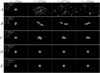 |
Fig. 1 Five different example simulations from GRAINS covering three different dynamical regimes, going from unstable or disaggregation in case A, different levels of reshaping in cases B–D, and stable in case E. The associated movies are available online. |
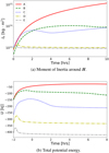 |
Fig. 2 Evolution of some of the global variables for the different exam ple simulations shown in Figure 1. |
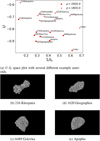 |
Fig. 3 Examples of how the shape and bulk density influences the dif ferent state variables. (a) The potential and moment of inertia around the angular momentum axis (in this case assumed to be the z-axis) for different asteroids and two different assumed bulk densities. (b–e) The rubble pile models of some of the asteroids used to calculate the state variable values. |
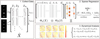 |
Fig. 4 Schematic illustration of the SINDy algorithm. A numerical derivative of the data from different GRAINS simulation are taken and put into a large data matrix |

3 Sparse identification of nonlinear dynamics
The SINDy algorithm was first developed in Brunton et al. (2016) with the aim to discover parsimonious dynamics from time series measurements of the system. It considers a dynami cal system described by an ordinary differential equation (ODE) of the form:
 (10)
(10)
where x ∊ ℝn is the state vector, β ∊ ℝp the static environment variable vector, and f (·) the dynamics of the system.
A general graphical description of the main steps of the SINDy algorithm are shown in Figure 4. The algorithm starts with the creation of a large data matrix X ∊ ℝ(m⋅k)×n consisting of snapshots of the state history x(t) at times t1,…, tm, for a set of k experiments each with a different set of environment parameters βi, i = {1,…, k}, as follows:
![$X = \left[ {\matrix{ {x_{{\beta _1}}^T\left( {{t_1}} \right)} \cr {x_{{\beta _1}}^T\left( {{t_2}} \right)} \cr \vdots \cr {x_{{\beta _1}}^T\left( {{t_m}} \right)} \cr {x_{{\beta _2}}^T\left( {{t_1}} \right)} \cr \vdots \cr {x_{{\beta _2}}^T\left( {{t_m}} \right)} \cr \vdots \cr {x_{{\beta _k}}^T\left( {{t_m}} \right)} \cr } } \right] = \left[ {\matrix{ {{x_{1,{\beta _1}}}\left( {{t_1}} \right)} & {{x_{2,{\beta _1}}}\left( {{t_1}} \right)} & \ldots & {{x_{n,{\beta _1}}}\left( {{t_1}} \right)} \cr {{x_{1,{\beta _1}}}\left( {{t_2}} \right)} & {{x_{2,{\beta _1}}}\left( {{t_2}} \right)} & \ldots & {{x_{n,{\beta _1}}}\left( {{t_2}} \right)} \cr \vdots & \vdots & \ddots & \vdots \cr {{x_{1,{\beta _k}}}\left( {{t_m}} \right)} & {{x_{2,{\beta _k}}}\left( {{t_m}} \right)} & \ldots & {{x_{n,{\beta _k}}}\left( {{t_m}} \right)} \cr } } \right].$](/articles/aa/full_html/2025/03/aa52432-24/aa52432-24-eq15.png) (11)
(11)
Afterwards, a function library is created which represents possible (nonlinear) terms which might be present in the dynam ics of the state variables. This function library is represented by the matrix  , where rx is the amount of library terms considered. An example of a function library is given in Eq. (12), where a combination of polynomials and trigonometric functions are chosen to be included:
![$\Theta (X) = \left[ {\matrix{ \mid & \mid & \mid & {} & \mid & \mid & \mid & {} \cr 1 & X & {{X^2}} & \ldots & {{X^d}} & {\sin (X)} & {X \cdot \sin (X)} & \ldots \cr \mid & \mid & \mid & {} & \mid & \mid & \mid & {} \cr } } \right].$](/articles/aa/full_html/2025/03/aa52432-24/aa52432-24-eq17.png) (12)
(12)
The monomial terms X(⋅) in Eq. (12) are defined as all possible combinations of the individual state variables up to order (·) at each snapshot, for example the first row of X2 is (ignoring β for ease of notation) ![${\left[ {x_1^2\left( {{t_1}} \right),{x_1}\left( {{t_1}} \right) \cdot {x_2}\left( {{t_1}} \right),{x_1}\left( {{t_1}} \right) \cdot {x_3}\left( {{t_1}} \right), \ldots x_2^2\left( {{t_1}} \right), \ldots x_n^2\left( {{t_1}} \right)} \right]^T}$](/articles/aa/full_html/2025/03/aa52432-24/aa52432-24-eq18.png) . There is a large amount of free dom in the selection of the specific library function, and the careful selection of library terms can improve the robustness of this method as the search space grows quickly if more library terms are included.
. There is a large amount of free dom in the selection of the specific library function, and the careful selection of library terms can improve the robustness of this method as the search space grows quickly if more library terms are included.
As this work considers parametric dynamics, additional terms for the β variables should be included in Θ. To remain as general as possible, a different set of library functions may be chosen for β compared to the function library of x. Thus, for each row of Θ(X), denoted by  , a tensor product is taken with the parameter function library
  :
:
 (13)
(13)
Stacking the feature libraries results in the final feature library Θ(X,β) ∊ ℝ(m⋅k)×r, where r = rx · rβ.
The final step of the SINDy algorithm is to find the correct combination of library terms that best represents the dynamics of the data. This is done by representing the dynamics as follows:
 (14)
(14)
where Ξ = [ξ1, ξ2,…, ξn] ∊ ℝr×n is the vector of coefficients rep resenting the importance of each individual function library term in the dynamics. The  is generally not directly available from the simulation, thus a numerical derivative of the data needs to be taken first. The coefficients in Ξ can be found by solving the following optimisation problem:
 (15)
(15)
where ||(·)||l represents the l-norm. Naively solving this problem will likely result in overfitting the data and a dynamical equation that does not hold outside the range of data provided to SINDy. Therefore, an l1 regularisation term is introduced to limit the magnitude of the coefficients and obtain sparse representation:
 (16)
(16)
where λ is a weight that can be tuned according to the amount of sparsity desired. This problem is solved in Brunton et al. (2016) using the sequential thresholded least squares (STLSQ) algorithm, which performs a least squares regression fit and after each fit zeroes out all the coefficients with magnitudes below a certain threshold. This will result in only a small amount of coefficients being non-zero, and thus a sparse representation of the dynamics. This also solves for redundancy in the function library terms (e.g. sin x can be included both directly or by its Taylor expansion in terms of monomials), but the sparsity regu- larisation term will always give preference to the least amount of terms. Other methods like the LASSO (Tibshirani 1996) or SR3 (Champion et al. 2019b) have also been shown to solve this type of regression problem well.
Besides reducing overfitting, promoting sparsity has other advantages. In Kutz and Brunton (2022), it is argued that promoting sparsity in data-driven dynamical systems is the best way of obtaining physical models. A parsimonious model is defined to have just enough complexity to describe the major components of the dynamics, and thus should identify the underlying dynamical mechanisms of the input data. Combining that with the ability to have a parametric dependency on relevant variables should produce a general model for the dynamics that is capable of predicting the evolution of initial conditions outside of the training dataset.
In Fasel et al. (2022), an extension to the normal SINDy algorithm was proposed, called library ensemble-SINDy (e-SINDy). In e-SINDy, a number of different models are generated from the same data, where for each model a part of the library terms are dropped from Θ(X,β). For each generated model, the coefficients are saved and at the end the median of all coefficients is used to generate the final model. This allows for the analysis of the probability distribution of each coefficient associated to a specific library term, and thus library terms with low inclusion probability, that is a associated coefficient with a probability close to zero, can be excluded. This not only makes the model more robust in case of high-noise levels and/or low amount of data, but also allows for an uncertainty quantification (UQ) associated with the final model.
4 Results and discussion
This section discusses the results of applying SINDy to the generated dataset from Section 2.2. The simulation dataset used here focuses on the effects of bulk properties like density and shape and how the change of shape due to increasing external forcing (i.e. increasing spin) is dependent on them. As the dataset spans different dynamical regimes, where the rubble pile may evolve both in a more fluid and solid like state, the capability to model the multi-regime nature of this system is tested. There are several other parameters that can be changed for these simulations, such as particle resolution, shape distribution, and contact parameters (here the damping and stiffness coefficients). To give an intuition of the effect of these parameters, simulations with several aggregates with different particle counts and size distribution were performed, which are shown in Figure 5. In short, increasing the amount of particles results in general in a shape that has more strength, as shown in Figure 5a. Similarly, Figure 5b shows that the monodisperse case is more robust against forcing due to the geometrical interlocking effect being more prominent, which is in agreement with previous studies like Zhang et al. (2021). The sensitivity to contact parameters is more complex and discussed in more detail in for example Hu et al. (2021).
As the goal of this study is to proof the effectiveness of SINDy in modelling this granular system, these parameters are kept constant across the simulations (see Appendix A for their values). This allows for a lower dimensional system which still exhibits the complexities of granular mechanics to be explored and thus for a simpler analysis and better understanding of the output of the methodology. The SINDy method allows for the inclusion of these parameters in β, thus no major changes to the proposed methodology are expected when including these parameters. Therefore, this investigation is left for future work.
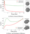 |
Fig. 5 Differences between aggregate simulation parameters. The top figure shows the difference between two different particle amounts, and the bottom shows the difference between using monodisperse and polydisperse particle sizes. |
4.1 SINDy accuracy
As discussed in Section 2.2, a large dataset is created for the generation of the e-SINDy dynamical model. Each simulation takes on average 45 minutes wall-clock time, on a system with an 13th Gen Intel(R) Core(TM) i7-13700 2.10 GHz CPU and 16 Gb of RAM. The dataset is separated into a training and testing set, with 80 percent of simulations used for the training set and 20 percent for the testing set. The data consists of the full 6 degree-of-freedom state of each particle in the simulation at each time step. Directly using these state variables with SINDy would result in a system of 6N equations of motion, which is numerically infeasible for SINDy and would result in the already known equations of motion for an individual particle given by Eqs. (2) and (3). Thus, a set of macroscopic coordinates need to be selected as state variables, which reduce the dimensionality of the problem and represent the large-scale state of the system well. Previous analytical models, as discussed in Section 2.1, have shown that amended potential ℰ plays a critical role in the dynamics of a finite-density N-body system. ℰ is calculated using two dynamical variables: Ih and U, together with the angular momentum H which remains constant over time. Thus, before the data is given to the e-SINDy algorithm all simulation data, consisting of different simulations with different values of H, is converted to a time-series of the state variables Ih and U using Eqs. (7) and (8). Thus, using the notation of Section 3, X = [Ih, U] and β = [H]. All state and environment variables are furthermore scaled to have an absolute maximum value of 1 for improved numerical performance.
The main variables that need to be selected for the e-SINDy algorithm are the sparsity regularisation parameter λ and the function library Θ. As discussed in the original SINDy paper Brunton et al. (2016), a monomial library has the most potential for the discovery of an accurate dynamical model when there is no prior physical information to aid the selection of the function library. After testing, it was found that constraining the function library associated to H to a maximum monomial degree of 2 produces the best results. This means that only the maximum monomial degree assosciated with the state variables Ih and U needs to be chosen. To select this and decide the value of λ, a set of models are created using a range of different values, λ = [1 e − 8,1.0], while also varying the maximum monomial degree present in the function library. Figure 6 shows the mean- squared error (MSE) for both the training and testing dataset as a function of the number of active coefficients (i.e. coefficients not thresholded away by the SINDy algorithm due to their low contribution to the equations of motion) in the found equations of motion. For lower λ and higher polynomial degrees, the number of active coefficients is higher as there are more potential terms in the function library and the sparsity weight is low. From Figure 6 it can be seen that only using linear terms is not sufficient, re-affirming the fact that the dynamics considered here are highly nonlinear. Including higher order terms in the function library significantly reduces the error but increases the complexity of the equations as well. To determine if the model is capable of accurately reproducing initial conditions outside the training data, the accuracy of the test set is also measured. Figure 6 and Table 1 present these accuracies and show that for the linear case, the testing set has a much worse performance; however, for the higher orders the training and testing accuracies are almost the same. Table 1 also shows the time it took for the solving of Eq. (16) by SINDy. It can be seen that there is an increase in time for higher orders and lower λ, but that even the longest duration is orders of magnitude quicker than running a single simulation. Thus, this shows that there is no over-fitting of the training data in most cases and that the computational complexity of SINDy is much lower than the running of individual simulations. Thus, generating a SINDy model from the data can be done at low numerical cost while still providing information on parameters that were not contained within the simulation dataset. From these results, a function library with maximum monomial degree of 3 is chosen together with λ = 0.5, as these values balance the complexity and accuracy of the final dynamical model well.
It is important to note that, ideally, if the underlying true dynamical model of this system is an ODE represented by a third order polynomial, including higher order terms in the function library should not change the discovered model, as SINDy would filter out these higher order terms. Clearly this does not happen here as a fifth order model has a higher number of active coefficients. This means that multiple models with different functional components are able to describe the same dynamics with similar accuracy for the system considered here. There are several ways this can be improved upon, for example: changing the state variables (see e.g. Champion et al. (2019a) where the optimal state variables and dynamical model are found in conjunction), adding other terms to the function library, and/or using other optimisation schemes for solving problem (Eq. (16)) (Champion et al. 2019b). This work is only concerned with finding a sparse and interpretable dynamical model that has sufficient accuracy to describe the different dynamical behaviours of this system. Determining if there is one true underlying analytical dynamical model and discovering it, can likely be achieved using (a combination of) the previously discussed techniques and an extensive tuning campaign. However, as this is not the main goal of this paper, this is left for future work.
The final dynamical model, found by the e-SINDy algorithm, is graphically shown in Figure 7a. The active coefficients associated to a specific monomial term are coloured for each of the two ODEs, where the colour represents their absolute value. The inverse of Ih is used as this turns the (0,0) coordinate to an attracting point for when the rubble pile disaggregates, instead of having the Ih term go to +∞ asymptotically. This was found to significantly improve the performance of the e-SINDy algorithm. Figure 7a shows that a significant amount of terms of the function library are non-active, meaning that a relatively sparse model is found.
As an important property of a data-driven dynamical model is its ability to model the different dynamical regimes well, it is important to consider how the accuracy of the e-SINDy model differs across these various regimes. The GRAINS dataset consists of simulations with different bulk densities, initial rotational rates, and initial shapes. For each of the density and rotational rate combinations, the average MSE of the nine different simulations (i.e. the nine different initial shapes for that combination of density and spin rate) is calculated. The results are shown in Figure 7. It can be seen that in general, the MSE remains constant as the bulk density and the rotational rate changes, showing a good accuracy across different regimes. The exception to this is the most stable case, P = 5.8 h, ρ = 2000.0 kg/m3, which has a lower accuracy compared to the other cases. This is likely due to the fact that for this case the time derivative is much closer to zero, meaning the numerical signal for e-SINDy is low compared to the other cases, which makes it harder for the algorithm to fit both.
The trajectories for the five different cases presented in Figure 1 are shown in Figure 8, where the solid lines are the true GRAINS simulations and the dashed lines are the e-SINDy results. This figure shows the capability of the model to capture the dynamical behaviour of these simulation well, together with predicting accurately the change in dynamics for different initial conditions and angular momenta H. Case A and B show that the e-SINDy model captures the large changes happening for the more unstable cases well, while for case C and D the initial change and return to stable behaviour is also present in the analytical model. As discussed previously, the stable case, case E, shows the lowest accuracy. However, the e-SINDy model does not present large changes or extremely different behaviour than expected for this case. Showing that the qualitative behaviour is still captured in the analytical model.
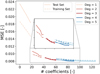 |
Fig. 6 Pareto front of e-SINDy models with different values of the maximum monomial degree and regularisation constant λ. The dashed lines represent the accuracy for the training set and the solid lines for the test set (i.e. simulations not contained in the e-SINDy training). |
Accuracy and computational time for different model parameters in mean squared errors (MSE).
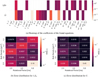 |
Fig. 7 Accuracy results for the e-SINDy model with degree 3 and λ = 0.5. |
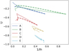 |
Fig. 8 Comparison of the predicted e-SINDy trajectory (dashed) versus the actual trajectory from GRAINS (solid) for the cases shown in Figure 1. |
4.2 Dynamical system analysis
As discussed before, one of the advantages of using SINDy is that it allows for the use of various tools and techniques from dynamical systems theory to be used on what was originally purely time series data. In this section, two examples of this are given. First, the vector field representing the flow of the system can be investigated for different parameter values, including the nullclines and equilibrium points. Second, coherent structures separating different regions of U−Ih space are determined using the finite time Lyapunov exponent.
The vector field in U−Ih space is plotted for different values of the angular momentum in Figure 9, where the arrows and their colour represent the direction and magnitude of the state derivative. The red and blue solid lines represent the nullclines, that is the regions where  and
and  , respectively. Thus, the intersections of these lines are the equilibrium points of this system. For all values of H, the (0,0) point is always found to be an attracting equilibrium point, as is expected as this point represents a breakup of the aggregate. For lower H, the nullclines dominate most of the U−Ih space and remain fairly close together, representing the small changes in shape happening for lower angular momenta. As the angular momentum increases, the nullclines and equilibrium points start to move to the lower left region of U−Ih space, which is the area where higher bulk density aggregates are located. Thus, the denser shapes remain more stable whereas the regions where lower density aggregates are located move towards the (0,0) equilibrium point, with an increase in the magnitude of the derivatives observed as well for these shapes. As H approaches zero, the U−Ih space is almost completely dominated by the flow moving towards the (0,0) point, and only high bulk density and closely packed shapes will not break up.
The U−Ih space can be further characterised by finding Lagrangian coherent structures (LCS), which are the most repelling, attracting, or shearing surfaces in phase space. They form surfaces that order the phase space into different regions with different dynamical behaviour. Various examples and a more in depth definition of LCS can be found in Haller (2015). There are various ways of determining the LCS in a system, see Hadjighasem et al. (2017) for a systematic comparison. In this work, the LCS are identified using the finite time Lyapunov exponents (FTLE), which are a type of chaos indicators which find the direction of maximum stretching of a region of initial conditions in phase space during a certain time interval. To calculate them, first the right Cauchy Green strain tensor was calculated as follows:
![$C\left( {{x_0}} \right) = {\left[ {\Phi _{{t_0}}^t} \right]^T}\Phi _{{t_0}}^t,$](/articles/aa/full_html/2025/03/aa52432-24/aa52432-24-eq28.png) (17)
(17)
where  is the state transition matrix (the linear flow of the system),
  is the flow map related to the dynamical system of Eq. (10) (i.e.
  ), and ∇ is the gradient operator. The FTLE was then defined as:
 (18)
(18)
where T = tƒ − t0, and λ is the largest eigenvalue of C(x0). This definition is the two-dimensional extension of the definition given in Ferrari and Alessi (2023). The LCS can then be identified by calculating the FTLE values for a large number of initial conditions and then finding the ridges of the FTLE field. The flow map and its gradient are hard to obtain, even for dynamical systems where an analytical estimate of the dynamics is available. Thus, the gradient was obtained numerically by propagating a set of trajectories using the e-SINDy model and calculating the derivatives as follows:
![$\nabla F_{{t_0}}^t\left( {{x_0}} \right) \approx \left[ {\matrix{ {{{I_h^{ - 1}\left( {t;{t_0},I_{h,0}^{ - 1} + {\delta _{{I_h}}}} \right) - I_h^{ - 1}\left( {t;{t_0},I_{h,0}^{ - 1} - {\delta _{{I_h}}}} \right)} \over {2\left| {{\delta _{{I_h}}}} \right|}}} & {{{I_h^{ - 1}\left( {t;{t_0},I_{h,0}^{ - 1} + {\delta _U}} \right) - I_h^{ - 1}\left( {t;{t_0},I_{h,0}^{ - 1} - {\delta _U}} \right)} \over {2\left| {{\delta _U}} \right|}}} \cr {{{U\left( {t;{t_0},{U_0} + {\delta _{{I_h}}}} \right) - U\left( {t;{t_0},{U_0} - {\delta _{{I_h}}}} \right)} \over {2\left| {{\delta _{{I_h}}}} \right|}}} & {{{U\left( {t;{t_0},{U_0} + {\delta _U}} \right) - U\left( {t;{t_0},{U_0} - {\delta _U}} \right)} \over {2\left| {{\delta _U}} \right|}}} \cr } } \right],$](/articles/aa/full_html/2025/03/aa52432-24/aa52432-24-eq33.png) (19)
(19)
where δi is a small perturbation in the ith coordinate direction.
An example of an FTLE map for the system identified in this work is given in Figure 10, where the different panels show different values of T. The colourmap shows clearly the ridge of maximum FTLE values as a yellow line, implying that this is an LCS (to be precise, a repelling LCS as these FTLE maps are calculated in forward time). To help interpret the maps further, the evolution of a set of initial conditions from a rectangular region at time t0 is also shown using blue dots. It can be seen in the FTLE maps that the rectangle of initial conditions is stretched nearly perpendicular to the FTLE ridge, one part of the rectangle moving below the ridge and the other above. This shows how the LCS separates the U−Ih space into regions with different behaviours. Important to note is the selection of the value for T, which here is taken to be at the end of the simulation (10 hours). For the case of Figure 10 it was found that for longer simulation times the relative FTLE values do not change significantly for longer simulation times. As such, it is assumed that this value for T is sufficient.
The change in the U−Ih space structure as the scaled angular momentum H changes can be quantified by the FTLE maps as well. This is shown in Figure 11, where the map for T = 10 hours is shown for eight different scaled angular momenta values. For each different value, the ridges can again clearly be seen by the yellow lines representing the highest FTLE values. For the lowest value of H, there are two main regions. First, the lower left region with the highest density asteroids have low FTLE values, representing relatively regular behaviour (labelled as stable in Figure 11). The other, larger, region has slightly higher FTLE values, meaning slightly more complex behaviour.
Comparing to the U–Ih space plot in Figure 9, this region contains nullclines and equilibrium points, showing that initial conditions here will move through the U−Ih space more, but likely end up in a stable shape instead of towards disaggregation. As the angular momentum increases, the larger region gets split into two different regions. The right region (labelled as reshaping in Figure 11) contains shapes that get elongated, and as the momentum increases, the ridge moves more to the left, meaning that more elongation is allowed. At around H = 0.75, the (0,0) equilibrium point is contained within this region and disaggregation becomes more likely for initial shapes in the right region (now labelled as disaggregation in Figure 11). The upper left region (labelled as quasi-stable for lower H and reshaping for higher H) is similar to the one described before, with several stable and unstable equilibrium points, leading to complex behaviour and also possible shape changes (and possibly disaggregation in medium to high H cases). This region also contains instances such as case B from Figure 1, which shows the detaching and re-attachment of parts of the aggregate, showing the complex shapes that are contained in that region.
Figure 11 also shows a set of white crosses, relating to the location in U−Ih space of the shapes of some known asteroids from Figure 3 (assuming a bulk density of 2000 kg/m3 ). This shows that most of these asteroids remain in the lower left stable region where there is little to no change in their shape, until the angular momentum crosses above the 0.6–0.7 region, where some are now contained in reshaping and disaggregation regions. This also shows that this transition happens at different points for different shapes, suggesting that certain shapes are more robust against changes in their spin states compared to others.
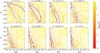 |
Fig. 9 Evolution of the U−Ih space as the angular momentum increases. The arrows represent the direction of the derivative and their colour representing the magnitude. The blue solid lines are the nullclines of U, the solid red lines the nullclines of 1/Ih, and the circles represent the equilibrium points. |
 |
Fig. 10 Finite time Lyapunov exponent maps over (simulation) time for a normalised angular momentum value of 0.6. The blue dots are a set of initial conditions that start from a rectangular region at time zero. The colourbars represent the value of the FTLE. |
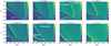 |
Fig. 11 Finite time Lyapunov exponent maps for different values of the angular momentum of the system. The white crosses represent the values for the different asteroids (with bulk density set to 2000 kg/m3) of Figure 3. |
5 Conclusion
In this work, a novel technique that is able to produce a sparse analytical dynamical model from data is used to analyse the shape dynamics of rubble pile asteroids. The data stems from a set of complex simulations of the gravitational and contact dynamics between a large amount of irregularly shaped particles, under different external conditions. The dynamical model was found to be accurate for the various different dynamical regimes considered here, only showing small inaccuracies under extremely stable conditions (i.e. very low rotational rates and high bulk densities). Even in those cases, the changes predicted by the model are very small, and thus the general qualitative behaviour is still captured well.
The discovered model showed that for small angular momenta, the U–Ih space contains several equilibirium points and nullclines, generally spread apart evenly. As the momentum increases, the U–Ih space becomes more dominated by the basin of attraction of the equilibrium point at the origin, representing the disaggregation of the asteroid. A similar analysis using Lagrangian coherent structures revealed that the U–Ih space can be separated into three different regions, each representing different dynamical behaviours, with their respective sizes changing as the angular momentum is increasing. This was validated by showing that the shapes of several real asteroids all fall inside the most stable region.
This work shows that SINDy is able to model various effects present in granular systems (e.g. nonlinear and multi-regime dynamics), thus being capable of providing insights into the dynamical behaviour of rubble pile asteroids. The equations of motion resulting from this method can be investigated using well known tools, such fixed point analysis and finite time Lyapunov exponents. Future studies can use the proof-of-concept of this methodology presented here to more extensively analyse the dynamical effects for other scenarios (e.g. YORP spin-up) and/or for other parameters (e.g. contact energy dissipation) to increase the knowledge of this complex dynamical system.
Data availability
Movies associated to Fig. 1 are available at https://www.aanda.org
Acknowledgements
The authors would like to thank the reviewer for their constructive comments which improved the manuscript greatly. Funded by the European Union (ERC, TRACES, 101077758). Views and opinions expressed are however those of the author(s) only and do not necessarily reflect those of the European Union or the European Research Council. Neither the European Union nor the granting authority can be held responsible for them.
Appendix A Simulation setup
A summary of the various settings used for the GRAINS simulation can be found in Table A.1. The selection of the dynamical parameters can depend on various properties of the granular materials. Here we use the values taken from the Fleischmann et al. (2016) and Ferrari et al. (2017) studies. Future experimental studies will be performed to further improve the estimates of these values (Vaghi et al. 2024).
Simulation initial conditions.
References
- Angelis, D., Sofos, F., & Karakasidis, T. E. 2023, Arch. Comput. Methods Eng., 30, 3845 [CrossRef] [Google Scholar]
- Arakawa, M., Saiki, T., Wada, K., et al. 2020, Science, 368, 18 [Google Scholar]
- Ballouz, R. L., Walsh, K. J., Sánchez, P., et al. 2021, MNRAS, 507, 5087 [NASA ADS] [CrossRef] [Google Scholar]
- Barnouin, O. S., Daly, M. G., Palmer, E. E., et al. 2019, Nat. Geosci., 12, 247 [Google Scholar]
- Barnouin, O. S., Ballouz, R. L., Marchi, S., et al. 2024, Nat. Commun., 15, 1 [Google Scholar]
- Brunton, S. L., Proctor, J. L., & Kutz, J. N. 2016, PNAS USA, 113, 3932 [NASA ADS] [CrossRef] [Google Scholar]
- Chambat, F., Vermersch, J., & Rambaux, N. 2023, A&A, 675, L2 [NASA ADS] [CrossRef] [EDP Sciences] [Google Scholar]
- Champion, K., Lusch, B., Nathan Kutz, J., & Brunton, S. L. 2019a, PNAS USA, 116, 22445 [NASA ADS] [CrossRef] [Google Scholar]
- Champion, K., Zheng, P., Aravkin, A. Y., Brunton, S. L., & Kutz, J. N. 2019b, IEEE Access, 8, 169259 [Google Scholar]
- Chandrasekhar, S. S. 1969, Ellipsoidal figures of equilibrium, Mrs. Hepsa Ely Silliman memorial lectures 1963 (New Haven: Yale University Press) [Google Scholar]
- Chapman, C. R. 1977, GCA, 40, 701 [NASA ADS] [Google Scholar]
- Chen, R. T. Q., Rubanova, Y., Bettencourt, J., & Duvenaud, D. K. 2018, in Adv. Neural. Inf. Process. Syst., 31 [Google Scholar]
- Dam, M., Brøns, M., Juul Rasmussen, J., Naulin, V., & Hesthaven, J. S. 2017, Phys. Plasmas, 24, 22310 [CrossRef] [Google Scholar]
- Fasel, U., Kutz, J. N., Brunton, B. W., & Brunton, S. L. 2022, Proc. R. Soc. A, 478 [CrossRef] [Google Scholar]
- Ferrari, F., & Alessi, E. M. 2023, A&A, 672, A35 [NASA ADS] [CrossRef] [EDP Sciences] [Google Scholar]
- Ferrari, F., & Tanga, P. 2020, Icarus, 350, 113871 [NASA ADS] [CrossRef] [Google Scholar]
- Ferrari, F., & Tanga, P. 2022, Icarus, 378, 114914 [NASA ADS] [CrossRef] [Google Scholar]
- Ferrari, F., Tasora, A., Masarati, P., & Lavagna, M. 2017, Multibody Syst. Dyn., 39, 3 [CrossRef] [Google Scholar]
- Ferrari, F., Lavagna, M., & Blazquez, E. 2020, MNRAS, 492, 749 [NASA ADS] [CrossRef] [Google Scholar]
- Fleischmann, J., Serban, R., Negrut, D., & Jayakumar, P. 2016, J. Comput. Nonlinear Dyn., 11 [Google Scholar]
- Fukami, K., Murata, T., Zhang, K., & Fukagata, K. 2021, J. Fluid Mech., 926, A10 [NASA ADS] [CrossRef] [Google Scholar]
- Hadjighasem, A., Farazmand, M., Blazevski, D., Froyland, G., & Haller, G. 2017, Chaos, 27 [CrossRef] [Google Scholar]
- Haller, G. 2015, Annu. Rev. Fluid Mech., 47, 137 [NASA ADS] [CrossRef] [Google Scholar]
- Hestroffer, D., Sánchez, P., Staron, L., et al. 2019, A&AR, 27, 1 [CrossRef] [Google Scholar]
- Hirabayashi, M. 2015, MNRAS, 454, 2249 [NASA ADS] [CrossRef] [Google Scholar]
- Hirabayashi, M., Kim, Y., & Brozovic, M. 2021, Icarus, 365, 114493 [NASA ADS] [CrossRef] [Google Scholar]
- Hoffmann, M., Fröhner, C., & Noé, F. 2019, J. Chem. Phys., 150, 25101 [NASA ADS] [CrossRef] [Google Scholar]
- Holsapple, K. A. 2001, Icarus, 154, 432 [NASA ADS] [CrossRef] [Google Scholar]
- Holsapple, K. A. 2004, Icarus, 172, 272 [NASA ADS] [CrossRef] [Google Scholar]
- Holsapple, K. A. 2007, Icarus, 187, 500 [NASA ADS] [CrossRef] [Google Scholar]
- Holsapple, K. A. 2010, Icarus, 205, 430 [NASA ADS] [CrossRef] [Google Scholar]
- Hu, S., Richardson, D. C., Zhang, Y., & Ji, J. 2021, MNRAS, 502, 5277 [NASA ADS] [CrossRef] [Google Scholar]
- Kirkpatrick, D. G., & Seidel, R. 1983, IEEE Trans. Inf. Theory, 29, 551 [CrossRef] [Google Scholar]
- Kutz, J. N., & Brunton, S. L. 2022, Nonlinear Dyn., 107, 1801 [NASA ADS] [CrossRef] [Google Scholar]
- Lai, Z., & Nagarajaiah, S. 2019, MSSP, 117, 813 [NASA ADS] [Google Scholar]
- Lauretta, D. S., DellaGiustina, D. N., Bennett, C. A., et al. 2019, Nature, 568, 55 [Google Scholar]
- Loiseau, J. C., & Brunton, S. L. 2018, J. Fluid Mech., 838, 42 [NASA ADS] [CrossRef] [Google Scholar]
- Lusch, B., Kutz, J. N., & Brunton, S. L. 2018, Nat. Commun., 9, 1 [NASA ADS] [CrossRef] [Google Scholar]
- Marohnic, J. C., DeMartini, J. V., Richardson, D. C., Zhang, Y., & Walsh, K. J. 2023, Planet. Sci. J., 4, 245 [NASA ADS] [CrossRef] [Google Scholar]
- Movshovitz, N., Asphaug, E., & Korycansky, D. 2012, ApJ, 759, 93 [NASA ADS] [CrossRef] [Google Scholar]
- Papastamatiou, K., Sofos, F., & Karakasidis, T. E. 2022, AIP Adv., 12, 25004 [NASA ADS] [CrossRef] [Google Scholar]
- Pravec, P., & Harris, A. W. 2000, Icarus, 148, 12 [NASA ADS] [CrossRef] [Google Scholar]
- Raducan, S. D., & Jutzi, M. 2022, Planet. Sci. J., 3, 128 [NASA ADS] [CrossRef] [Google Scholar]
- Richardson, D. C., Walsh, K. J., Murdoch, N., & Michel, P. 2011, Icarus, 212, 427 [Google Scholar]
- Rozitis, B., Maclennan, E., & Emery, J. P. 2014, Nature, 512, 174 [CrossRef] [Google Scholar]
- Sánchez, P., & Scheeres, D. J. 2011, ApJ, 727, 120 [CrossRef] [Google Scholar]
- Scheeres, D. J. 2012, CMDA, 113, 291 [NASA ADS] [CrossRef] [Google Scholar]
- Scheeres, D. J. 2016, in Recent Advances in Celestial and Space Mechanics, 23 (Cham: Springer), 31 [CrossRef] [Google Scholar]
- Scheeres, D. J. 2020, CMDA, 132, 1 [CrossRef] [Google Scholar]
- Scheeres, D. J., & Brown, G. M. 2023, CMDA, 135, 1 [CrossRef] [Google Scholar]
- Scheeres, D. J., Hartzell, C. M., Sánchez, P., & Swift, M. 2010, Icarus, 210, 968 [NASA ADS] [CrossRef] [Google Scholar]
- Schmidt, M., & Lipson, H. 2009, Science, 324, 81 [CrossRef] [Google Scholar]
- Sunday, C., Murdoch, N., Tardivel, S., Schwartz, S. R., & Michel, P. 2020, MNRAS, 498, 1062 [NASA ADS] [CrossRef] [Google Scholar]
- Tancredi, G., Maciel, A., Heredia, L., Richeri, P., & Nesmachnow, S. 2012, MNRAS, 420, 3368 [NASA ADS] [CrossRef] [Google Scholar]
- Tasora, A., & Anitescu, M. 2010, J. Comput. Nonlinear Dyn., 5, 1 [Google Scholar]
- Tasora, A., Serban, R., Mazhar, H., et al. 2016, in High Performance Computing in Science and Engineering, 9611 (Springer Verlag), 19 [Google Scholar]
- Tibshirani, R. 1996, J. R. Stat. Soc. Series B Stat. Methodol., 58, 267 [CrossRef] [Google Scholar]
- Vaghi, S., Fodde, I., & Ferrari, F. 2024, in The 7th International Conference on Multibody System Dynamics, Madison, WI, USA [Google Scholar]
- Vlachas, P. R., Byeon, W., Wan, Z. Y., Sapsis, T. P., & Koumoutsakos, P. 2018, Proc. R. Soc. A: Math. Phys. Eng. Sci., 474 [Google Scholar]
- Watanabe, S., Hirabayashi, M., Hirata, N., et al. 2019, Science, 364, 268 [NASA ADS] [Google Scholar]
- Yoshikawa, M., Fujiwara, A., & Kawaguchi, J. 2006, Proc. Int. Astron. Union, 2, 401 [CrossRef] [Google Scholar]
- Zhang, Y., Michel, P., Richardson, D. C., et al. 2021, Icarus, 362, 114433 [CrossRef] [Google Scholar]
All Tables
Accuracy and computational time for different model parameters in mean squared errors (MSE).
All Figures
|
Fig. 1 Five different example simulations from GRAINS covering three different dynamical regimes, going from unstable or disaggregation in case A, different levels of reshaping in cases B–D, and stable in case E. The associated movies are available online. |
| In the text | |
|
Fig. 2 Evolution of some of the global variables for the different exam ple simulations shown in Figure 1. |
| In the text | |
|
Fig. 3 Examples of how the shape and bulk density influences the dif ferent state variables. (a) The potential and moment of inertia around the angular momentum axis (in this case assumed to be the z-axis) for different asteroids and two different assumed bulk densities. (b–e) The rubble pile models of some of the asteroids used to calculate the state variable values. |
| In the text | |
|
Fig. 4 Schematic illustration of the SINDy algorithm. A numerical derivative of the data from different GRAINS simulation are taken and put into a large data matrix |
| In the text | |
|
Fig. 5 Differences between aggregate simulation parameters. The top figure shows the difference between two different particle amounts, and the bottom shows the difference between using monodisperse and polydisperse particle sizes. |
| In the text | |
|
Fig. 6 Pareto front of e-SINDy models with different values of the maximum monomial degree and regularisation constant λ. The dashed lines represent the accuracy for the training set and the solid lines for the test set (i.e. simulations not contained in the e-SINDy training). |
| In the text | |
|
Fig. 7 Accuracy results for the e-SINDy model with degree 3 and λ = 0.5. |
| In the text | |
|
Fig. 8 Comparison of the predicted e-SINDy trajectory (dashed) versus the actual trajectory from GRAINS (solid) for the cases shown in Figure 1. |
| In the text | |
|
Fig. 9 Evolution of the U−Ih space as the angular momentum increases. The arrows represent the direction of the derivative and their colour representing the magnitude. The blue solid lines are the nullclines of U, the solid red lines the nullclines of 1/Ih, and the circles represent the equilibrium points. |
| In the text | |
|
Fig. 10 Finite time Lyapunov exponent maps over (simulation) time for a normalised angular momentum value of 0.6. The blue dots are a set of initial conditions that start from a rectangular region at time zero. The colourbars represent the value of the FTLE. |
| In the text | |
|
Fig. 11 Finite time Lyapunov exponent maps for different values of the angular momentum of the system. The white crosses represent the values for the different asteroids (with bulk density set to 2000 kg/m3) of Figure 3. |
| In the text | |
Current usage metrics show cumulative count of Article Views (full-text article views including HTML views, PDF and ePub downloads, according to the available data) and Abstracts Views on Vision4Press platform.
Data correspond to usage on the plateform after 2015. The current usage metrics is available 48-96 hours after online publication and is updated daily on week days.
Initial download of the metrics may take a while.