| Issue |
A&A
Volume 618, October 2018
|
|
|---|---|---|
| Article Number | A113 | |
| Number of page(s) | 42 | |
| Section | Stellar atmospheres | |
| DOI | https://doi.org/10.1051/0004-6361/201833235 | |
| Published online | 23 October 2018 | |
Searching for the weakest detectable magnetic fields in white dwarfs⋆
Highly-sensitive measurements from first VLT and WHT surveys
1
Armagh Observatory and Planetarium, College Hill, BT61 9DG Armagh, UK
e-mail: stefano.bagnulo@armagh.ac.uk
2
University of Western Ontario, London, N6A 3K7 Ontario, Canada
e-mail: jlandstr@uwo.ca
Received:
14
April
2018
Accepted:
18
July
2018
Our knowledge of the magnetism in white dwarfs is based on an observational dataset that is biased in favour of stars with very strong magnetic fields. Most of the field measurements available in the literature have a relatively low sensitivity, while current instruments allow us to detect magnetic fields of white dwarfs with sub-kG precision. With the aim of obtaining a more complete view of the incidence of magnetic fields in degenerate stars, we have started a long-term campaign of high-precision spectropolarimetric observations of white dwarfs. Here we report the results obtained so far with the low-resolution FORS2 instrument of the ESO VLT and the medium-resolution ISIS instrument of the WHT. We have considered a sample of 48 stars, of which five are known magnetic or suspected magnetic stars, and obtained new longitudinal magnetic field measurements with a mean uncertainty of about 0.6 kG. Overall, in the course of our survey (the results of which have been partially published in papers devoted to individual stars) we have discovered one new weak-field magnetic white dwarf, confirmed the magnetic nature of another, found that a suspected magnetic star is not magnetic, and suggested two new candidate magnetic white dwarfs. Even combined with data previously obtained in the literature, our sample is not sufficient yet to reach any final conclusions about the actual incidence of very weak magnetic fields in white dwarfs, but we have set the basis to achieve a homogeneous survey of an unbiased sample of white dwarfs. As a by-product, our survey has also enabled us to carry out a detailed characterisation of the ISIS and the FORS2 instruments for the detection of extremely weak magnetic fields in white dwarfs, and in particular to relate the signal-to-noise ratio to measurement uncertainty for white dwarfs of different spectral types. This study will help the optimisation of future observations.
Key words: magnetic fields / polarisation / white dwarfs
The spectra are only available at the CDS via anonymous ftp to cdsarc.u-strasbg.fr (130.79.128.5) or via http://cdsarc.u-strasbg.fr/viz-bin/qcat?J/A+A/618/A113
© ESO 2018
1. Introduction
During the past century, observations have gradually established that magnetic fields can be directly detected, usually through the Zeeman effect, in some (but not all) stars in most of the major phases of stellar evolution. Evolutionary stages in which stellar magnetic fields have been detected include the T Tau and Herbig AeBe phases, the main sequence (upper and lower), and the red giant, AGB, white dwarf, and neutron star phases (Donati & Landstreet 2009; Bagnulo & Landstreet 2015). Thus, the potential importance of magnetic fields extends over most of the observable HR diagram.
The incidence and the typical strength and morphology of the magnetic field are different for different kinds of stars. In most of the cases, the origin of the magnetic field is not understood, and we do not know how fields evolve as stars evolve. At an even more basic level, the situation is that we simply do not understand why magnetic fields occur in some stars but not in others. In this situation, exploratory observations can play an important role by establishing clearly the circumstances in which magnetic fields are found, the strength and surface geometry of the fields, and the statistics of field occurence as a function of such parameters as stellar mass, age, and rotation, during various evolutionary phases.
In this and forthcoming papers we focus on the incidence of magnetic fields in the most common final stage of stellar evolution, that of white dwarfs (WDs). During this phase, we observe that a rather small fraction of stars (of the order of 10%, e.g. Landstreet et al. 2012) exhibit surface magnetic fields. These fields range in global field strength from a few kG to nearly 103 MG. Most of the known fields have strengths between roughly 1.5 MG and 75 MG (which may be due to observational bias, see Sect. 2).
The fields observed in WDs do not appear to change their intrinsic structure on an observable time scale, and seem to be of fossil nature (that is, fields inherited from an earlier stage of evolution; for a review on the possible mechanisms that may have generated a magnetic field, including the merging of a binary system, see Ferrario et al. 2015). In principle, the rotation period of a magnetic white dwarf (MWD) may be determined from variation of the appearance of the field on the visible hemisphere of the star as it rotates; and modelling of the shape of spectral lines, particularly of the effect of the magnetic fields on these lines, may make it possible to obtain an approximate map of the surface structure of the stellar magnetic field. This has been attempted for a number of MWDs with some, but not complete, success (Jordan 1992; Euchner et al. 2002, 2006).
At present, the observational situation for WD magnetism still leaves a number of questions for which the answers should help to stimulate and improve our theoretical ideas about how the observed fields arise and evolve. (1) We do not yet have a clear picture of the frequency of occurence of magnetic fields of various strengths in either magnitude or volume limited WD samples. In particular, is the relative deficit of large and small fields relative to the 1.5 − 75 MG range of field strengths (Ferrario et al. 2015) real, or is it an artefact of selection effects in the discovery process? (2) We do not know if fields occur that are larger than 109 G or less than about 5 kG. (3) We do not know how the frequency of occurence of fields varies with WD mass or age, although there are hints that magnetic WDs may be more massive than the average, and that magnetic fields may be more common in cooler, older WDs than in hot, young stars (Liebert & Sion 1979; Liebert et al. 2003). (4) We have no information on how the surface structure of magnetic fields may vary with WD age or mass.
The observational data currently available do not provide sufficient constraints to any of these issues (see e.g. Ferrario et al. 2015), mainly because of two reasons: (1) the weak-field regime is probed only by a small fraction of the relevant measurements, or, in simpler words, the large majority of magnetic field strength measurements available in the literature have rather large uncertainties; and (2) the database of available measurements is quite inhomogeneous in both space distribution and stellar parameters.
To improve this situation, ideally we need a large survey of WD magnetism aimed at a complete coverage of a volume-limited region of space, with uniform field detection thresholds. The survey volume should be large enough to establish with statistical precision the incidence of magnetism as a function of mass and age.
In practice, there are major problems with completing such a survey. Even within a distance of 20 pc from the Sun it is thought that the known sample of about 140 WDs is still missing about 20 undiscovered stars (Holberg et al. 2008, 2016), whose absence will clearly affect statistical conclusions. A certain number of the WDs that are within such a volume are nevertheless old enough (more than about 5 Gyr) and cool enough (Teff < 5000 K) that some are fainter than V ∼ 17. Such stars require the use of the largest telescopes to acquire the necessary normal or polarised spectra, but the field detection threshold would still be substantially higher than in case of V = 13 or 14 stars. A third problem is that the sensitivity of (spectro-) polarimetry to the detection and measurement of fields varies considerably from WDs with a strong line spectrum (DA, DB, DZ stars) for which uncertainties smaller than 1 kG can be obtained, to stars lacking any optical atomic spectral lines (DC, DQ stars), for which the practical uncertainties are of the order of 1 MG or larger. To the best of our knowledge, the only attempt to conduct a volume-limited sample study of the incidence of magnetism was made by Kawka et al. (2007), who considered a volume within 13 pc thought to be complete by Holberg et al. (2002).
An alternative approach would be to observe a magnitude-limited sample, which, however, would very strongly favour hot, young WDs, and certainly would be a poor representation of the local WD population (and obviously would still have the problem of insensitivity to the fields of DC stars). In practice, all the surveys undertaken so far have effectively been magnitude-limited surveys, and the best possible approach, especially now that the Gaia parallaxes are made available, will be to collect new data that complement the existing ones towards the completion of a volume-limited sample, while being aware fully aware of the various observational biases.
To inform the strategy of future surveys, we need first to assess the degree of completeness of the available observations of WDs. In Sect. 2 we present a short review the main characteristics and the results of the surveys carried out so far, which will be a starting point to establish our criteria for target selection in this and forthcoming survey papers. Regarding the choice of the instrument for our surveys, over the past 50 years or so, several different techniques have been used to measure magnetic fields in WDs. Their detection limits depend not only on signal-to-noise ratio (S/N) but also on the spectral characteristics of the star, and this will be discussed in Sect. 3. For our survey we have used the FORS2 instrument of the European Southern Observatory’s Very Large Telescope (ESO VLT), the ISIS instrument of the William Herschel Telescope (WHT), a low-resolution and a mid-resolution spectropolarimeter, respectively, and the high-resolution spectropolarimeter ESPaDOnS of the Canada-France-Hawaii Telescope (CFHT). In this paper we present the results obtained so far with the FORS2 and ISIS spectropolarimeters. More details on the FORS2 and ISIS instruments and the settings used in this survey are given in Sect. 4. Our observing strategy was aimed in part at assessing the reliability of the instruments (in particular of ISIS, which is less commonly used in spectropolarimetric mode than FORS2), and our experiments are described in Sect. 5. Data reduction is described in Sect. 6. The results of our tests, including quality checks, are given in Sect. 7. The results of our observations of scientific targets are given in Sect. 8. In Sect. 9 we consider the relative sensitivity of magnetic field detections as obtained with the two different instruments, and as a function of the spectral types of the WDs. In Sect. 10 we discuss our scientific results, and in Sect. 11 we summarise our conclusions.
2. Previous surveys of magnetic fields in WDs
Techniques employed for detection and modelling of magnetic fields in WDs are optical spectroscopy, broad-band polarimetry, and spectropolarimetry, and the quantitative data interpretation depends on the field strength. The simplest case is when field strength is ≲1 MG. In this regime, the continuum is not detectably polarised, and the Stokes profiles of spectral lines may be interpreted in terms of the linear Zeeman effect. In this regime, detection and modelling of magnetic fields in WDs is very similar to that carried out for non-degenerate stars (e.g. Mathys 1989; Donati & Landstreet 2009; Bagnulo & Landstreet 2015). For field strengths in the range ∼1 to 50 MG, spectral lines are formed in the quadratic Zeeman regime, and line polarisation and splitting may be interpreted in terms of field strength with the aid of numerical computations of the atomic structure of H and He (e.g. Kemic 1974). For field strengths ≳50 MG, the magnetic field polarises the continuum (Kemp 1970), and the various components of the spectral lines may be shifted by several hundred Å, or are washed out so completely as to become indistinguishable from the continuum. The estimate of the field strength rely again on numerical atomic computations (Wunner et al. 1985). In all regimes, as a general rule, unpolarised spectroscopy is sensitive to the field strength averaged over the visible stellar disk, or mean field modulus ⟨|B|⟩; circular polarisation is sensitive to the longitudinal component of the magnetic field, again averaged over the visible stellar disk, and called the mean longitudinal field ⟨Bz⟩. Linear polarisation is sensitive to the field transverse components, but is far less commonly employed as a diagnostic tool than the other techniques. Below we summarise the outcome of the main surveys for magnetic fields in WDs carrried out in the last 60 years.
2.1. Early non-detections of WD fields
During the 1960’s, extensive spectroscopy of WDs (particularly that carried out by J. L. Greenstein, for example Eggen & Greenstein 1965), made it clear that WDs with H or He line spectra (DA or DB white dwarfs) show in general no sign of magnetic splitting. Based on a sample of more than 100 DA and DB stars observed with a typical spectral resolving power of several hundred (typically with dispersion of 190 Å mm−1, Eggen & Greenstein 1967), no indication was found that large fields having ⟨|B|⟩ of the order of a MG or more occur in WDs. The threshhold of this general absence of fields was quantitatively estimated by Preston (1970), who showed that, based on a sample of about 20 DA WDs, “few if any WDs... have surface magnetic fields as large as 5 × 10⁵ G”.
The first survey of WDs for still weaker magnetic fields (a project suggested by L. Woltjer) was made by Angel & Landstreet (1970b), using interference filters with a photoelectric polarimeter to isolate the wings of the Hβ line in DA stars, searching for Zeeman-effect induced circular polarisation in these line wings. This survey reached uncertainties in ⟨Bz⟩ of the order of 30 kG for nine WDs, but detected no fields.
2.2. First discoveries and early successful surveys
The discovery of the first magnetic WD was made by Kemp et al. (1970) by means of broad-band circular polarimetry. This approach was stimulated by Kemp’s theory (Kemp 1970) that a field of the order of 107 G at the surface of a WD would cause broad-band continuum circular polarisation of the optical radiation. This idea turned out to be qualitatively correct, and led to the discovery of a field of many MG in the white dwarf Grw+70°8247 (= WD 1900+705). It was quickly discovered that the radiation of this MWD is also linearly polarised (Angel & Landstreet 1970a), and eventually it was shown that the field of this star is in the 100s of MG range (Angel et al. 1985). Grw+70°8247 still has one of the strongest MWD fields known.
Further surveys, mostly looking for broad-band circular polarisation, gradually uncovered roughly 1–2 MWDs per year: G195-19 (Angel & Landstreet 1971a), G99-37 (Landstreet & Angel 1971), G99-47 (Angel & Landstreet 1972), etc. The first clear indication of magnetic variability was observed in the 1.33 d periodic variation of circular polarisation in the light of G195-19 (Angel & Landstreet 1971b). For the first 20–25 years of magnetic investigations of WDs, most MWDs were detected and studied using broad-band optical circular polarisation (see e.g. Angel et al. 1981; Landstreet 1992), but it was also realised that Zeeman splitting of Balmer lines by magnetic fields is rare in WDs, but not absent (e.g. G99-47 and Feige 7, Liebert et al. 1975, 1977). Combining all field detections and non-detection of the first decade together, Angel et al. (1981) concluded that the probability of finding a magnetic field of between 3 106 and 3 108 G in a WD is at least 3%.
2.3. More recent spectropolarimetric surveys
Schmidt & Smith (1995) carried out a spectropolarimetric survey of 170 DA stars brighter than B = 15 to search for fields below roughly 1 MG. The method used was to search for the circular polarisation produced in the wings of Balmer lines by the presence of a non-zero mean longitudinal field ⟨Bz⟩. This method is very similar in principle to that of Angel & Landstreet (1970b); however, the use of a low-resolution (R ∼ 700) spectropolarimeter allowed both Hα and Hβ to be observed simultaneously. The mean error bar σ⟨Bz⟩ was 8.6 kG, but 7 targets were re-observed with long exposure times to achieve σ⟨Bz⟩ ≲ 2 KG. This survey discovered four new MWDs, bringing the total number of MWDs known at that time to 42 (see Table 2 of Schmidt & Smith 1995).
Putney (1997) observed 46 isolated WDs classified as DCs in the WD catalogue by McCook & Sion (1987) for spectrally resolved circular polarisation. Her survey used spectral coverage from 3700 to 8000 Å with spectral resolving power R ∼ 400. She found that many of her targets were misclassified: of the 46 DC WDs, only 22 are genuine DC stars. Most of the remaining ones are DA stars with very weak Hα and almost no other visible Balmer series lines. Fields were detected in five faint stars (V ∼ 16 − 17), two of which still need to be confirmed by further observations.
A spectropolarimetric survey of 61 bright DA white dwarfs in the southern hemisphere, with similar field measurement uncertainties as those of Schmidt & Smith (1995), was reported by Kawka et al. (2007). This survey reported marginal evidence of a field in WD 0310−688, which was not confirmed by later observations. At the time of their survey, Kawka et al. (2007) were able to list approximately 170 known MWDs. The abrupt increase in the total number of known MWDs was due to the first impact of wholesale discovery of WD fields in the range of ⟨|B|⟩ ∼ 2 to 80 kG by the Sloan Digital Sky Survey (SDSS; see Sect. 2.6 below.)
Kawka & Vennes (2012) carried out a magnetic survey of some 58 high proper motion DA white dwarfs using ESO FORS1 and FORS2 with uncertainties σ⟨Bz⟩ of typically a few kG. These stars tend to be relatively cool (the median value of Teff is about 6500 K). Kawka & Vennes (2012) discovered a previously unknown magnetic field in one DAZ star of Teff ≈ 6000 K, and may have found a weak field in a cool DA star (NLTT 347); they also discovered magnetic variability in two previously unknown cool, MG-field WDs.
Vornanen et al. (2010), 2013 carried out a small survey of 11 DQ (C-rich) WDs for magnetic fields, and found a field of ⟨Bz⟩ ≈ 1.5 MG in WD 2153−512 = GJ 841B, a rare C-rich WD with CH bands. It appears that cool WDs with atomic or molecular metal lines may be a fruitful category of WD to search for weak fields, but such stars are usually rather faint, and the molecular Swan bands of C2 in the visible are extremely insensitive to magnetic fields.
2.4. Searching for extremely-weak fields in WDs
Two papers based on small spectro-polarimetric surveys of WDs with the VLT brought attention to the possibility that a large number of WDs may have a magnetic field that is not strong enough to be detected with in the previous low-resolution spectroscopic surveys. Aznar Cuadrado et al. (2004) and Jordan et al. (2007) used FORS1 to observe samples of 12 and 10 WDs respectively, with typical ⟨Bz⟩ error bars of 1 kG, and found respectively 3 and 1 new MWDs, each of which has a longitudinal field of only a few kG. The conclusion from these papers was that the rate of weak-field MWD was actually relatively high, perhaps up to 25%. However, one of the MWDs detected by these two studies was previously identified as a candidate magnetic star in a high-resolution spectroscopic survey (see Sect. 2.5), and one was not confirmed. When these two stars are removed from the survey statistics, the discovery frequency is similar to that found in other studies.
A similar survey of six DA stars and one sdO star by Valyavin et al. (2006) using the low-resolution prime focus UAGS spectropolarimeter at the 6-m BTA telescope at the Special Astrophysical Observatory yielded marginal evidence for a field in WD 1105−048. This field was still not fully confirmed in spite of numerous further measurements (but see Sect. 10 in this paper).
Landstreet et al. (2012) presented the results of another small VLT spectropolarimetric survey focussed on 10 relatively cool WDs, with a typical ⟨Bz⟩ error bar between 1 and 1.5 kG. They detected a field in a WD which Koester et al. (1998) had flagged as possibly magnetic, but considered also the possibility that the Hα line core is broadened by rotation. Landstreet et al. (2012) revised the data reductions of earlier FORS1 samples of 36 WDs with high-precision field measurements, showing that some of the previous marginal detections obtained with FORS1 were probably spurious. Landstreet et al. (2012) concluded that WDs with very weak magnetic fields are not much more common than WDs with strong and very strong magnetic fields.
Recent VLT spectropolarimetric field measurements of five DAZ stars, most with ⟨Bz⟩ uncertainties σ⟨Bz⟩ below 1 kG, are reported by Farihi et al. (2018), but fields were found only in the two WDs that were already known to be magnetic from previous measurements (see Sect. 2.5).
2.5. High-resolution spectroscopic surveys
In Sect. 2.1 we noted that the first large survey for MG magnetic fields, with negative results, was effectively carried out by classification spectroscopy in the 1960s. More recently, high-resolution spectroscopy has been found to be a tool that is effective for searching for MWDs with fields of some tens of kG or more.
Koester et al. (1998) reported detection of three new MWDs with ⟨|B|⟩ fields in the kG range from close examination of high-resolution (flux) spectra of a sample of WDs, taken to find evidence of rotation by searching for rotational broadening of the core of Hα. High resolution spectroscopy of WDs was continued within the framework of the ESO Supernova Ia Progenitor Survey (SPY) project, a search for close SB2 white dwarf pairs (possible SN Ia progenitors) with the ESO UVES spectrograph. SPY was the first project for which a substantial sample of WDs was systematically observed with high spectral resolving power (R ∼ 18 000 − 80 000). The SPY survey confirmed that such observations provide, as a side product, a powerful method of detecting not only magnetic fields in the 1–100 MG range, but that the sensitivity extends down to mean surface fields ⟨|B|⟩ of the order of 50 kG, which can be detected via Zeeman splitting in the core of the Hα line. Still weaker fields, down to about 20 kG, broaden the core of the Hα line significantly, but to distinguish this from rotational broadening, spectropolarimetry is required.
Based on SPY data, Koester et al. (2001, 2009) identified several further MWDs with ⟨|B|⟩ below 1 MG. Because fields as weak as ⟨|B|⟩ ∼ 50 kG will generally have longitudinal fields ⟨Bz⟩ below 15 kG, this is a field detection method almost as powerful as sensitive spectro-polarimetric surveys of Sect. 2.4.
High-resolution spectroscopic studies of DAZ WDs by Zuckerman et al. (2011) and Farihi et al. (2011) revealed sub-MG fields in two cool stars via detection of the Zeeman effect in the metal lines. Another cool DAZ was found to have a sub-MG field by Kawka & Vennes (2014), who point out that four of the 13 known cool (Teff < 7000 K) DAZ stars are not only magnetic, but have sub-MG fields. This is a very high fraction compared to estimates of the weak-field magnetic WDs in the general WD population of the order of 5%.
2.6. Discoveries of large magnetic field white dwarfs from the Sloan Digital Sky Survey
Until early in this century, magnetic WDs were discovered at a rate of at most a few per year. The rate of discovery of magnetic WDs increased dramatically as a result of the Sloan Digital Sky Survey, a huge project searching for and measuring the redshifts of millions of nearby galaxies. As a byproduct, this project has revealed roughly 30 000 new WDs, of which several hundred host magnetic fields (Schmidt et al. 2003; Külebi et al. 2009; Kleinman et al. 2013; Kepler et al. 2015, 2016; see also the summary of Ferrario et al. 2015). However, the rate of discovery of MWDs with fields below about 1 MG is still only one or two per year.
The data produced by the SDSS project are qualitatively different from those resulting from earlier studies. The MWDs discovered in earlier surveys are mostly among the brighter WDs, with magnitudes of 13 < V < 16. Many of these stars have been observed multiple times, often at relatively high S/N and/or high spectral resolution. The fields detected range over five orders of magnitude, from a few kG up to nearly 103 MG. In contrast, the MWDs discovered in the SDSS are mostly in the brightness range between V = 16 and V = 20. The spectra, taken with the low resolving power of R ∼ 1800, have low S/N, usually ≲20. Because of the low S/N and R, the threshold for detecting fields is roughly 2 MG, and field strengths can only be usefully estimated for the better spectra. In conclusion, this enormous increase in the number of known magnetic WDs has mainly increased our knowledge about the 2–80 MG range of the ⟨|B|⟩ field strength distribution, and the newly discoverd MWDs can mostly only be studied further using the largest telescopes.
2.7. The scope of our new surveys
The total sample of known MWDs, single and in binary systems, was recently analysed by Ferrario et al. (2015). Among the approximately 250 best-characterised magnetic WDs, only about 30 are known with fields (⟨Bz⟩ or ⟨|B|⟩) below 1 MG, and a slightly smaller number with fields ⟨|B|⟩ ≳ 80 MG; about 80% of well-characterised magnetic WDs have fields in the range of 1.5–80 MG.
Because of the difficulty of identifying the largest fields in DC or nearly DC spectra, and the lack of sensitivity to the weakest fields in most general surveys of WDs, it is unlikely that this distribution represents the true frequency of very low and very high fields. The considerably higher relative frequency of kG fields found in surveys sensitive to them, as discussed above, implies that there should still be a substantial number of such weak-field magnetic WDs to be discovered even among relatively bright (V less than 15 or 16) WDs. Thus, a survey to find more weak-field WDs has the potential to substantially improve our knowledge of the actual distribution of magnetic field strengths among WDs, to provide more bright examples of weak-field stars for detailed modelling and analysis, and to assist us in understanding whether magnetic fields decay during white dwarf cooling or whether some process(es) generate new magnetic flux. Our survey target list was originally based on a magnitude-limited sample, in order to better understand the capabilities and limitations of FORS2 and (especially) ISIS, and on the desire to monitor some of the MWDs that were discovered to be variable. The target lists of our future surveys will be aimed mainly at surveying a volume-limited sample of WDs such as the 20 or 25-pc samples described by Holberg et al. (2016), and will certainly benefit from the April 2018 release of new high-precision astrometry from the Gaia mission.
3. Magnetic field detection techniques: threshold and accuracy
On the base of the large body of experiment and experience applied to detect and measure fields in MWDs, we summarise here the strengths and limitations of the various methods.
3.1. Broad-band circular polarimetry
Broad-band circular polarimetry is sensitive in practice only to magnetic fields with typical strength ⟨Bz⟩ larger than roughly 10 MG, which are usually able to polarise the continuum at a detectable level (above about 0.1% polarisation) regardless of the spectral type. These measurements may be interpreted in terms of longitudinal field through the relationship between ⟨Bz⟩ in MG and circular polarisation in % (Kemp 1970) (1)
(1)
Equation (1) is actually little more than an order of magnitude estimate, and often underestimates the actual field as determined by modelling by a factor of order 10 (for example, compare the polarisation and ⟨|B|⟩ data in Table 2 of Landstreet 1992).
3.2. Circular spectropolarimetry
Circular narrowband or spectro-polarimetry of spectral lines is sensitive to the mean longitudinal field ⟨Bz⟩, with a sensitivity that is determined by the signal-to-noise (S/N) that may be reached with current telescopes: practically, with current mid- to large-size telescopes, of a few hundred G in bright (V ∼ 13) DA stars. The threshold field sensitivity depends on the nature of the stellar spectrum, but polarisation may be detected in H Balmer lines, He and/or metal lines even when Zeeman splitting is negligible compared to the intrinsic line broadening (see Sect. 6). The detection threshold of the mean longitudinal magnetic field also depends on the instrument spectral resolution. There is no upper limit to the magnetic field that may be detected with circular polarimetry, because at the field regimes at which the magnetic fields washes out spectral features, the continuum is certainly polarised (see Sect. 3.1). We note that since spectro-polarimetry resolves the WD intensity spectrum to a greater or lesser extent, depending on the spectral resolution, the same data may be used to measure ⟨|B|⟩ if the field is large enough for the Zeeman splitting to be significantly larger than the spectral resolution element (see Sect. 3.3 below).
3.3. High-resolution spectroscopy
The mean magnetic field modulus ⟨|B|⟩ may be measured from the Zeeman splitting of spectral lines observed in intensity. The sensitivity of this technique increases with spectral resolution, but there is a lower limit to the value of ⟨|B|⟩ that can be detected that is set by the intrinsic broadening of the line cores of the lines used. It is a little difficult to specify the typical threshhold field above which high-resolution spectroscopy can reliably detect a field, as this depends on the field geometry (whether the geometry leads to a well-defined Zeeman triplet or not) and S/N, as well as the spectral class. However, for the commonest case of spectra of DA stars, we may take observation as a guide, and note that the (estimated) ⟨|B|⟩ ≈ 42 kG field of WD 2105−820 (Landstreet et al. 2012) does not lead to a clear Zeeman pattern in the core of Hα, while the 60 kG field of WD 2047+372 (Landstreet et al. 2017) does. Based on this, we estimate that the available high-resolution spectra of the WDs that show no clear Zeeman splitting provide upper limit of ⟨|B|⟩ ≲ 50 kG to possible fields. Spectroscopy may become less useful in the presence of fields above 80 MG, when spectral lines sometimes nearly disappear, as they do for G195-19 (Greenstein et al. 1971). Obviously, Zeeman splitting cannot be measured in DC stars, which have no spectral lines, and in which a magnetic field may be detected with circular polarimetric techniques only if strong enough to measurably polarise the continuum.
3.4. Accuracy of the field measurements
Regardless of the sensitivity that may be achieved in the measurement of polarisation, and the accuracy quoted for derived measurements such as ⟨Bz⟩ and ⟨|B|⟩ that are obtained with the various techniques, it is essential to recall that the interpetation of the actual I and V/I spectra in terms of ⟨Bz⟩ and ⟨|B|⟩ relies on simplifying assumptions that are not very accurate. The adopted transformations may lead to precise values for the field strengths, but the precise meaning of these values is rarely clear. The result is that different methods of field strength measurement, and even measurements with the same techniques in different wavelength regions, may lead to field strength values that differ by much more than the nominal uncertainties. This does not invalidate the usefulness of these field values for estimating the strength of observed fields, but indicates that caution is required in interpreting them. The issue has recently been discussed in some detail with respect to field measurements of main sequence stars using FORS1 by Landstreet et al. (2014), and we comment on it again in Sect. 7.1.
4. Instruments and instrument settings of our survey
Both ⟨|B|⟩ and ⟨Bz⟩ measurements are needed for simple dipole modelling of the stellar magnetic structure, using the customary modelling techniques historically applied to Ap and Bp stars (e.g. Landstreet & Mathys 2000; Bagnulo et al. 2002a; Landstreet et al. 2017). However, even for detection purpose, it is useful to have both high-resolution I and V/I spectra, since there are examples of MWDs with large ⟨|B|⟩ values with little or no signal of circular polarisation (e.g. WD 2359−434, Landstreet et al. 2017), or, viceversa, with no clear indication of Zeeman splitting but with a measurable signal of circular polarisation in spectral lines (e.g. WD 0446−789, Aznar Cuadrado et al. 2004).
Based on these considerations, it is clear that the ideal instrument to detect magnetic fields in WDs would be a high-resolution spectropolarimeter that can accurately measure both continuum and line polarisation. Being fibre-fed, high-resolution spectropolarimeters lack accuracy in the determination of polarisation in the continuum, so the best viable option is a multi-instrument approach that makes use of both low- and mid-resolution spectropolarimetry (with capabilities in the continuum) and mid- to high-resolution spectroscopy or spectro-polarimetry of spectral lines. Based on these considerations we have decided to use the FORS2 instrument of the ESO VLT, the ISIS instrument of the 4.2 m WHT of the Issac Newton Group (ING), and the high-resolution spectropolarimeter ESPaDOnS at the Canada-France-Hawaii Telescope (CFHT).
The first two instruments are those used in this survey, and are briefly described in the following paragraphs. In a forthcoming paper we will report survey results obtained with ESPaDOnS.
Both FORS2 and ISIS have polarimetric optics arranged according to the optical design described by Appenzeller (1967). The polarimetric module consists of an achromatic retarder waveplate (λ/2 for observation of linear polarisation, or λ/4 for observation of circular polarisation) which can be rotated to a series of fixed positions, followed by a beam splitting device: a Wollaston prism in the case of FORS2, and a Savart plate in case of ISIS. Essentially, these devices split the incoming radiation into two beams polarised in directions perpendicular to each other, one along the principal plane of the plate (the parallel beam f‖), and one perpendicularly to that plane (the perpendicular beam f⊥). The beams split by the Wollaston prism are tilted at an angle of about 20°, while the beams split by a Savart plate propagate parallel to each other but separated. A Wollaston mask (Scarrott et al. 1983) or a special dekker prevents the superposition of each beam split by the beam splitter with the light coming from the other parts of the observed field of view.
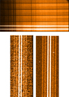 |
Fig. 1. Raw image of spectropolarimetric data obtained with FORS2 (top panel), ISIS blue CCD (bottom left panel) and ISIS red CCD (bottom right panel). For all images, the dynamic range is set to show the sky background, which is at the level of a few hundred ADUs (while the spectra are at the level of several thousand ADUs). The FORS2 image refers to WD 2039−202 observed on 2015-06-02. The ISIS image refers to WD 2111+498 observed on 2015-08-30. For display purpose, the images of the ISIS spectra have been trimmed in the dispersion direction. Note in ISIS images the four strips illuminated by sky background. |
4.1. FORS2
FORS2 (FOcal Reducer Spectrograph) is a multi-purpose instrument capable of imaging and low-resolution spectroscopy in the optical, equipped with polarimetric optics. It is attached at the Cassegrain focus of Unit 1, Antu, of the ESO VLT of the Paranal Observatory. The instrument is described in Appenzeller & Rupprecht (1992) and Appenzeller et al. (1998). A raw spectropolarimetric image obtained with FORS2 is shown in the upper panel of Fig. 1. In our survey we used grism 1200B, which, with a dispersion of 0.71 Å per pixel (2 × 2 rebinning), covers the spectral range 3700–5200 Å. We used a 1″ slit width for a spectral resolving power of 1400. A discussion about the best choice for spectral range is presented in Sect. 9.2.
Currently, the FORS2 calibration plan includes regular monitoring of standard stars for linear polarisation, but does not include a regular check of the λ/4 waveplate. However, the polarimetric optics are fixed in one of the instrument wheels, and need not be realigned when they are used. It is probably safe to assume that the correct alignment of the λ/4 retarder waveplate may be monitored from occasional measurements of well known magnetic stars obtained within a few months. For instance, the well known magnetic Ap stars HD 94660 and HD 188041 were observed in 2015 and 2016 and the measured values of the field were in agreement with previous literature values (Bagnulo et al. 2017b).
4.2. ISIS
The Intermediate dispersion Spectrograph and Imaging System (ISIS) is mounted at the Cassegrain focus of the 4.2 m WHT. The instrument is equipped with polarimetric optics, and the use of dichroic filters permits simultaneous observing in two arms (blue and red), covering different spectral regions.
The observations in the blue arm were obtained with grating R600B, centred at λ = 4400 Å, for a dispersion of 0.44 Å per pixel. Most of the observations were carried out with a 1″ slit width, but for a few cases, under some less ideal seeing conditions, we widened the slit to 1.2″, or even 2.0″ (for four observations). Spectral resolving power, as measured near the central wavelength on the lines of the arc lamp, was about 2600, 2200 and 1250 for slit widths of 1.0″, 1.2″ and 2.0″, respectively. In the red arm we employed grating R1200R centred at λ = 6500 Å, with 0.26 Å per pixel. Observations were mostly made with a 1.0″ slit width, and only in a few occasions with a 1.2″ slit width. Spectral resolving power measured at the central wavelength with slit widths 1.0″ and 1.2″ was 8600 and 7200, respectively. Five measurements in the red arm were obtained with grating R158R (dispersion = 1.8 Å per pixel) with a 1.0″ slit width, for a spectral resolving power of 1100.
4.2.1. Alignment of the polarimetric optics
The alignment of the retarder waveplate of ISIS is checked during the afternoon before the first night of observations by inserting a linear polariser in the optical beam, and finding at which angles of the retarder waveplate the contrast between the fluxes measured in the two beams is minimum or maximum. This way, the instrument scientist measures the offset α0 between the zero position of the encoders, and the angle between the one of the axes of the retarder waveplate and the ordinary beam of the Savart plate. It is then left to the user to set the retarder waveplate at the correct positions separated by 90° to measure the reduced Stokes parameter V/I.
4.2.2. The use of the dichroic in spectropolarimetric mode
Observations may be carried out simultaneously in the red and blue arm by inserting a dichroic, or in one arm at a time, by inserting a mirror (when observing in the blue arm)1 or leaving the optical path free (in which case only the red arm is fed). We note that in the two different arms the positions of the ordinary and extra-ordinary beam are swapped (due to the different direction of the readout of the two CCDs in the two arms). Without taking this into account, the polarisation of the same object observed in the two arms would be measured with opposite sign.
ISIS documentation warns that “using a dichroic is not recommended for spectropolarimetric observations due to the reflected light from its rear. The reflected light is displaced along the slit, partly into the spectrum of the other polarisation, which may compromise the polarimetry measurements”. To investigate this problem, we carried out some experiments in linear polarimetric mode, and observed some discrepancy between observations obtained in the same arm with and without dichroic. We originally thought that these discprepancies could be ascribed to scattered light due to the presence of the dichroic, and we decided to use only one arm at a time (mainly the blue arm). Later, we discovered that these discrepancies had probably an alternative explanation, linked to an inaccurate positioning of the retarder waveplate, as discussed by Bagnulo et al. (2017a) regarding FORS2 measurements. Therefore in our second run we decided to experiment with the use of the dichroic in circular polarimetric mode. Two magnetic stars, HD 157751 and γ Equ, were observed simultaneously in both arms with the dichroic; then, immediately afterwards, in the blue arm and in the red arm individually. The results of our experiments, presented in Sect. 7.2, showed us that the use of the dichroic does not have any impact on our field measurements. Therefore in our August 2015 run we proceeded with simultaneous observations in the blue and in the red arm. Among the five available dichroics we used the standard one with cut-off centred at 5300 Å.
5. Observing strategy and tests
Our new observations were carried out with the FORS2 instrument of the ESO VLT in service mode between March and September 2015 (during semester P95) and between April and July 2016 (during semester P97), and with the ISIS instrument of the 4.2 m WHT of the ING during two dedicated observing runs in visitor mode, in February 2015 and in August 2015 (during semesters 15A and 15B, respectively). Prior to these observing runs, four field measurements of three WDs were obtained with ISIS in January 2014 as a pilot experiment, and two stars were observed with FORS2 as a backup programme. In total we have observed 48 WDs. Twelve of these stars were observed more than once, and the total number of new spectropolarimetric observations of WDs is 79. Science targets and observations are discusssed in later Sections. Here we discuss more technical aspects of our campaign.
5.1. Observations of well known magnetic stars to check ISIS performance
During our WHT observing runs we frequently checked the instrument performance. A reliable way to do this is to observe bright stars with well known magnetic fields. The most obvious candidates are the magnetic Ap/Bp stars of the main sequence, many of which have been well studied in the past. Ap/Bp stars usually have variable magnetic fields, but their variability is often well known, and prediction can be made for the expected field values ⟨Bz⟩ and sometimes ⟨|B|⟩ at a given epoch. The reference stars that we used in our survey are HD 65339 (= 53 Cam), HD 157751, HD 201601 (= γ Equ) and HD 215441 (Babcock’s star). Below we describe the characteristics of the magnetic fields of these stars; the comparison with our observations will be made in Sect. 7.1.
5.1.1. HD 65339
HD 65339 is a extremely well studied magnetic stars with a longitudinal magnetic field that changes from +4500 to −4600 (as measured using an Hβ photoelectric polarimeter) with a rotation period of P = 8.02681 ± 0.00004 d. The zero point of the ephemeris refers to the magnetic maximum HJD = 2448498.186 ± 0.022, and the mean longitudinal field curve may be fit by (2)
(2)
with B0 = −53 G and B1 = 4572 G (Hill et al. 1998).
5.1.2. HD 157751
HD 157751 is a star discovered as magnetic by Hubrig et al. (2006). It is not clear if its field is variable, but it was observed because it has a strong field and could serve for the purpose of comparing field measurements with and without dichroic (see Sect. 4.2.2).
5.1.3. HD 201601
HD 201601 = γ Equ has a fairly strong magnetic field with an extremely long rotation period, of the order of a century; Bychkov et al. (2016) report a rotation period of P = 35462.5 ± 1150 d, refer the rotation phase to the positive cross-over on HJD = 2425176.5, and provide for Eq. (2) the coefficients B0 = −265 G and B1 = 850 G. At the time of our observations of this star, the nominal value of ⟨Bz⟩ ≈ −745 G.
5.1.4. HD 215441
With a mean field modulus of about 35 kG, Babcock’s star HD 215441 is the star with the strongest magnetic field known among Ap stars. The field measurements available in the literature do not allow us to calculate the rotation period: the mean field modulus is nearly constant, while only a few longitudinal field measurements are available. Therefore we rely on the photometric ephemeris brightness in the B filter, P = 9.487574 ± 0.000030 d, with a light maximum at HJD = 2448733.714 (North & Adelman 1995), and on a qualitative correlation between field strength and star brightness: by comparing data of Borra & Landstreet (1978) with the light curve of Leckrone (1974) we find that the magnetic maximum occurs close to maximum brightness. From a fit to the Hβ data by Borra & Landstreet (1978) we find B0 = 15 700 G and B1 = 4800 G.
5.2. Zero field measurements
In a few experiments we also observed reference stars after setting the retarder waveplate at position angles such that the polarisation signal should be zero, that is, we set the retarder waveplate at position angles of 0° and 90° instead of ±45° with respect to the principal axes of the beam splitter. Any non–zero field resulting from this experiment would point either to a misalignemnt of the retarder waveplate or to instrument flexures (for a discussion on how instrument flexures may lead to spurious detections see Bagnulo et al. 2013). We call these measurements “Zero field measurements” to distinguish them from the null field, i.e., the field estimate that one would obtain by using the null profiles instead of the V/I profiles (for definition and discussion of the use of the null profiles and the null fields, see Bagnulo et al. 2012, 2013).
5.3. The effect of a small offset of the retarder waveplate
The possibility to set the retarder waveplate at an arbitrary position angle allowed us to perform some experiments, namely: to experimentally check if and how the measured value of the longitudinal magnetic field changes for small deviations of the position of the retarder waveplate from the nominal values, and to check that after offsetting the positions of the retarder waveplate by 45°, one actually measures a null polarisation signal (and a magnetic field consistent with zero) even in strongly magnetic stars. We also measured the magnetic field of two reference stars, HD 215441 and γ Equ, after systematically offsetting the position angle of the retarder waveplate by ±5deg, and compared the results with the measurements obtained without this artificial offset. The results of these experiments are described in Sect. 7.
6. Data reduction
Steps for data reduction are similar for both FORS2 and ISIS instruments. After bias-subtraction, background subtraction, flux extraction and wavelength calibration, we obtained the reduced Stokes V profiles (PV = V/I) by combining the various beams according to the well known formulas (3)
(3)
where f‖ and f⊥ are the flux measured in the parallel and perpendicular beam of the beam splitter device, respectively (e.g. Bagnulo et al. 2009), and αi = 315° or 135° (in the large majority of cases we had N = 4 and αi = 315°). The uncertainty of the PV profile in a certain spectral bin is approximately given by S/N−1, where the S/N is accumulated in that spectral bin adding up the fluxes measured in both beams at all positions of the retarder waveplate (e.g. Bagnulo et al. 2009).
In the Zeeman regime, field measurements may be obtained by using the technique described by Bagnulo et al. (2002b), i.e., by minimising the expression: (4)
(4)
where, for each spectral point i, yi = V(λi)/I(λi), and b is a constant introduced to account for possible spurious polarisation in the continuum, geff is the effective landé factor, and (5)
(5)
where e is the electron charge, me the electron mass, and c the speed of light. An extensive discussion of these techniques is provided by Bagnulo et al. (2012). For this survey we have adopted the same σ clipping algorithm used by Landstreet et al. (2012), but also decided to clean the spectra from cosmic-rays using the relevant option in the IRAF apall procedure. In some cases, especially those with the longest exposure times, this has allowed us to decrease the uncertainties of our measurements. Our spectral analysis is shown in Fig. A.1, which are organised as follow. In the upper panel, the black solid line shows the intensity profile, the shape of which is heavily affected by the transmission function of the atmosphere + telescope optics + instrument. The red solid line is the V/I profile (in % units) and the blue solid line is the null profile offset by −2.25% for display purpose. Photon-noise error bars are also centred around −2.25% and appear as a light blue background. Spectral regions highlighted by green bars have been used to detemine the ⟨Bz⟩ value from H Balmer lines. The two bottom panels show the best-fit obtained by minimising the expression of Eq. (4) using the V/I profiles (left panels) and the NV profiles (right panels).
6.1. Determining the sign of Stokes V
Field measurements of the reference stars are crucial not only to check instrument performance, but also, at a very basic level, to establish the correct sign of the Stokes V profiles (hence, of the magnetic field).
The sign of V can be obtained via analytical formulas once the orientation of the polarimetric optics is known. However, getting the PV profile with the correct sign from these “first principles” is a challenging task. One needs to identify which of the parallel and perpendicular beams of the beam splitter device illuminates which image on the CCD (remembering that, for ISIS, red and blue CCDs are read out in different ways, and that therefore the position of the parallel and perpendicular beams are swapped in the red and blue arms). Then one has to be sure of the convention used by the software package of preference regarding the naming of the aperture (i.e., whether aperture number increases towards the left or towards the right). Each of these issues may well be gotten under control, but there is no doubt that a comparison of the field measurement of a reference star with the expected value from previous literature studies represents an attractive short-cut to determine the correct sign of our field determination, and this is the method that we have used. In summary, our determination of the sign of the V profile was guided by the goal to make the sign of the longitudinal magnetic field measured for our reference stars consistent with the value expected from previous literature data.
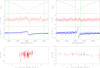 |
Fig. 2. Hβ (left panel) and Hα (right panel) lines of star WD 1840−111 observed with ISIS in the blue and red arm, respectively. Top panel: I profile (in arbitrary units). Second panel from top: V/I profile. Third panel from top: x = −Cz λ2(1/I)dI/dλ vs. wavelength. The green vertical lines show the wavelength intervals in which the x values clearly depart from zero, and which have been choosen to apply the least-square technique. Bottom panel: relation between V/I and x for the points within the solid green lines in the upper panels. Note that the x and V/I ranges of the Hβ plots are half the size of the corresponing ranges in the Hα plots. |
6.2. Measurements in the Hα profile
It is important to note that the Hα profile is often affected by fringing issues (in the case of ISIS) and water vapour features, and, less often, by features due to a WD or dMe companion, like the double degenerate WD 0135−052 (Saffer et al. 1988) and the WD+dMe system WD 1213+528, or non ideal background subtraction (the solar spectrum may pollute the target spectrum in observations obtained during full moon nights or during twilight, if the background is not accurately subtracted). These spurious signals clearly have a negative impact on the field measurements, and in a subtle way. While photon noise scatters V/I along the y direction, fringing and water vapour features scatter the points along the x direction, invalidating the use of a least squares technique under the approximation that the errors on x are much smaller than the errors on y. Practically, these issues are effectively indistinguishable from the contribution of spectral lines showing no polarisation, and they dilute the field (if present) while still formally adding precision to the measurements. Figure 2 shows that this situation is mitigated by considering only the core of Hα, where I is sufficiently steep that fringing issues becomes negligible with respect to photon-noise.
7. Test results and quality checks
7.1. Magnetic field measurements of the reference stars
The values of the field measurements of the reference stars of Sect. 5.1 allow us to perform a first basic quality check of our observations and to find the sign of our Stokes V measurements.
HD 65339 was observed during our January 2014 run at rotation phase ∼0.9 and during our February 2015 runs at various rotational phases from ∼0.1 to ∼0.5. The remaining reference stars were all observed during our August 2015 run. Table A.1 shows the observing log of the magnetic reference stars, and the measured magnetic field.
We found that all our field measurements of magnetic Ap stars are broadly consistent with the field value predicted by simple sinusoidal curves based on their known rotation period, (Fig. 3 shows the case of 53 Cam) but with some discrepancies that have various explanations. First of all, we note that high S/N measurements of γ Equ and 53 Cam that were obtained during a short interval of time (a few minutes) with identical instrument settings are sometimes inconsistent with their (small) errorbars. Similarly, Table A.2 shows the results of high S/N observations obtained with the retarder waveplate at 0° and 90°, which depart from zero by much more than can be explained by photon-noise. This suggests that, as in the FORS spectrograph (Bagnulo et al. 2012), small flexures create spurious signals that become important when photon-noise is very low. This interpretation is confirmed by the fact that if we consider the high S/N measurements of the Ap stars, the distribution of the null field values normalised by their error bars departs from a Gaussian distribution with σ = 1.
Simultaneous or quasi-simultaneous observations of the same Ap star in two different arms show remarkable discrepancies, and so do the field measurements obtained from H Balmer lines and those obtained from He and metal lines. This phenomenon is well known and discussed by Landstreet et al. (2014). The quantity ⟨Bz⟩ is conceptually an average of the line-of-sight component of the surface magnetic field over the visible hemisphere, but which average? It is clear that the surface does not emit the same specific intensity in the direction of the observer from every surface element (for example, due to limb darkening), and also that the spectral lines in which the polarisation is measured do not have exactly the same shape and strength over the whole visible hemisphere (lines tend to weaken mildly towards the limb). Thus the hemispheric average of the longitudinal field is weighted somewhat towards the centre of the visible disk. This weighting will vary with wavelength, and from one line to another (due to the details of line formation). The result is that we can confidently expect that values of ⟨Bz⟩ determined in different wavelength regions, or with different spectral lines, will have similar magnitudes but will frequently differ from one another by considerably more than the nominal uncertainties imply. This is the case for the measurements we report. The discrepancies between the fit to previous measurements and our new datapoints seen in Fig. 3 are also to be ascribed to the fact that the ephemeris of 53 Cam is not accurate after a time interval of 20 years.
Another important point to keep in mind is the following. The technique we use here for deducing the value of ⟨Bz⟩ from a polarised spectrum is valid in the “weak-field” limit, where the splitting of the components of the Zeeman multiplet is small compared to the natural width (as convolved with the spectrograph profile) of the line. In general, this assumption is valid. An obvious exception are the ⟨Bz⟩ measurements of HD 215441 with ISIS using the R1200R grating. In this case many line components are close to being resolved by the instrument, and the peaks of the polarisation no longer coincide with the global line wings, but with the centres of the Zeeman σ components. Thus the proportionality between large V/I and large line slope in I is broken and the value of ⟨Bz⟩ is underestimated.
Finally, another implicit assumption of this method is that the spectral lines are mostly well separated from neighbours. In the cases of metal lines of red spectra of HD 215441 obtained with grating R1200R, and of both H Balmer and metal lines of HD 65339 obtained with the R158R grating, the resolving power is so small that many lines are blended together with near neighbours. Again the proportionality of V/I with dI/dλ is broken, and the field is underestimated. The case of HD 215441 was discussed in detail by Landstreet et al. (2015). For the remaining cases, the ⟨Bz⟩ values should be realistic estimates of field on the observed stellar hemisphere. For a more fundamental discussion of these points, see Landstreet (1982) or Mathys (1989).
Table A.1 includes also the results of some observations obtained with the retarder waveplate delibrately offset by ±5°, immediately before or after observations obtained with the retarder waveplate set in the correct position. Bagnulo et al. (2009) showed that deviations from the nominal values of the position angle of the retarder waveplate are compensated to first order by the beam swapping technique (in circular polarisation only); their Fig. 3 shows that a systematic offset of 5° would introduced a relative error on Stokes V/I of about 1%. In HD 215441, we see that field measurements are within error bars, confirming the expectation that a misaligment as small as 5° does not significantly alter the field measurements. More significant differences are seen on the field measurements of HD 201601, which are characterised by a much higher S/N, and may be ascribed again to instrument flexures.
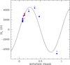 |
Fig. 3. Comparison of our ISIS measurements of reference star 53 Cam = HD 65339 with the sinusoidal curve obtained by Hill et al. (1998). Filled circles refer to measurements obtained from metal lines, and empty squares to field measurements from H Balmer lines. Blue symbols refer to data obtained with grating R600B, and red symbols to data obtained with the R1200R grating. Error bars are shown only for the measurements obtained from H Balmer lines; their size is comparable to the symbol size. |
7.2. The impact of using a dichoric on the circular polarisation measurements
Table A.1 includes also the results of the observations of reference stars obtained simultaneously in the red and in the blue arms, and (quasi-simultaneosuly) in the red and in the blue arm separately, as explained in Sect. 4.2.2; the differences in field measurements obtained when observing in one arm at a time and with dichroic actually agree surprisingly well within photon-noise error bars. Furthermore, when comparing the PV profiles, we did not discover significant discrepancies beyond those due to photon-noise. In conclusion, we found that the dichroic could be used without affecting our measurements.
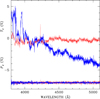 |
Fig. 4. First-order effects of imperfect flat-fielding that are in fact canceled out by adopting the beam-swapping technique. The solid thick blue line refers to FORS2 data (with grism 1200B), the thin solid red line to ISIS data (grating R600B). Offset by −7% (for display purpose) are the PV profiles obtained with the beam swapping technique. |
7.3. The spurious polarisation removed by the beam-swapping technique
The beam swapping technique removes the instrumental polarisation introduced by the polarimetric optics (see Bagnulo et al. 2009). It is of some interest to check how much is the contribution that would be introduced mostly by imperfect flat-fielding (see Eq. (34) of Bagnulo et al. 2009). This can be calculated simply by replacing  in Eq. (3) with the expression
 (6)(see also Maund 2008; Ilyin 2012). Figure 4 compares examples taken from FORS2 and ISIS observations, and shows that the quantity
  is much higher (in absolute value) and much more wavelength dependent in FORS2 observations than in ISIS observations. This exercise suggests that in cases of ISIS, spectropolarimetric observations obtained with just at one position of the retarder waveplate may still be useful, perhaps after a normalisation to the continuum. The impact of imperfect flat-fielding in FORS2 data is such that data obtained at just one position of the retarder waveplate are difficult to correct.
7.4. Distribution of the null field measurements
Figure 5 shows the histogram of the ratio between null field and its error bar (in the ideal case it should be a Gaussian distribution with σ = 1). This histogram is obtained considering all FORS2 and ISIS measurements. When ISIS observations were obtained simultaneously in the red and in the blue ISIS arm, the ⟨Nz⟩ estimate is obtained by combining the two spectra. The distribution appears generally well within 3 σ and has only just a few outliers. It is not affected by instrument flexures because spectral lines of WDs are broad and photon-noise error bars are relatively high.
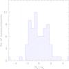 |
Fig. 5. Distribution of the ⟨Nz⟩ measurements normalised by their error bars for the WD observations. |
8. Results
We have obtained 79 ⟨Bz⟩ field measurements of 48 different WDs, 12 of them observed twice or more. With FORS2, we obtained 27 observations of a total of 13 stars (one of which is featureless, for which we could only rule out the presence of a field strong enough to polarise the continuum). With ISIS, we obtained 54 polarisation spectra of 38 stars (three targets were in common with the VLT sample). Twenty-four ISIS observations were obtained simultaneously in the blue and red arm, 25 observations were obtained only with in the blue arm, and five in the red arm only (four of them on the same star, with the low resolution grating R158R).
The log of the observations of WDs and the field measurements are given in Table A.3 (spectra of an additional star, WD 1900+705, will be presented in a forthcoming paper). All our spectra (Stokes I and V/I profiles) are made available at CDS. We note that some of our target WDs are also spectro-photometric standard stars with absolute fluxes tabulated in literature. For example, WD 0501+527 = BD+52 913 = G 191-B2B (Oke 1990; Bohlin 1995) was observed simultaneously in both ISIS arms (using the dichroic); WD 0549+158 = GD 71 (Bohlin 1995; Moehler et al. 2014), was observed in both ISIS arms with the dichroic; WD 1134+300 = GD 140 (Massey et al. 1988; Massey & Gronwall 1990) was observed with ISIS blue arm (with mirror insertion in the optical path); WD 2032+248 = HD 340611 = Wolf 1346 (Massey et al. 1988; Massey & Gronwall 1990), was observed in both ISIS arms with the dichroic; WD 0310−688 = GJ 127.1 = EG 21 (Hamuy et al. 1992) was observed with FORS2 / grism 1200B. The spectra of these stars may be used for an approximate flux calibration of all our targets, neglecting the effects due to slit losses. Airmass extinction coefficients for La Palma and for Paranal are given by King (1985) and Patat et al. (2011), respectively.
Table A.3 includes distances obtained from the most recent Gaia release (Gaia Collaboration 2018), and spectral types taken from Simbad database. In some cases we have adopted a more accurate spectral classification (DAZ) than that listed in Simbad (DA); these cases are WD 1116+026 (Xu et al. 2014), WD 1202−232 (Zuckerman et al. 2003), WD 1337+705 (Holberg et al. 1997; Zuckerman et al. 2003), WD 1632+177 (Zuckerman et al. 2003) and WD 2105−820 (Koester et al. 2005, 2009). We also note that Gaia distances are generally known with much better accuracy than what is shown in Table A.3, but higher accuracy is not important in the context of this work.
In addition, because of a typo in our target list, we obtained two observations of an sdOp star with the blue arm of ISIS, and because of a mistake from our side in the preparation of the observations, for two stars observed with FORS2 we obtained only intensity spectra. The log of these observations is given in Table A.4.
Figure 6 shows the distribution of the error bars of all FORS2 and ISIS ⟨Bz⟩ measurments. As in the case of Fig. 5, observations obtained simultaneously in the ISIS blue and red arm were combined together. This figure shows that the large majority of our new observations have an uncertainty smaller than 1 kG. The mean uncertainty of all field measurements of our survey is 0.6 kG.
In the course of the surveys presented in this paper we detected a magnetic field in six WDs: WD 2359−434 (observed with FORS2, already discovered as magnetic by Koester et al. 1998 and by Aznar Cuadrado et al. 2004), WD 0446−789 (observed with FORS2, already discovered as magnetic by Aznar Cuadrado et al. 2004), WD 1105−048 (observed with FORS2 and ISIS, already suspected as magnetic by Aznar Cuadrado et al. 2004), WD 2047+372 (observed with ISIS, detected as magnetic through Zeeman splitting in Hα, and discussed already by Landstreet et al. 2016, 2017), WD 2051−208 (observed with FORS2, already discovered as magnetic by Koester et al. 2009), WD 2105−820 (suggested as possibly magnetic from spectroscopy by Koester et al. 1998 and confirmed with FORS1 spectropolarimetry by Landstreet et al. 2012). In addition, we have obtained a single marginal field detection at about the 3σ level in two white dwarfs: WD 1031−114, a DA1.9 WD, and WD 2138−332, a DZ WD within the 20-pc volume around the Sun. Neither of these detections is at a sufficiently high level of significance to convince us that we have detected kG-level fields in these stars, so further observations of each will be undertaken. In particular, we note that some high-resolution (but low S/N) spectra obtained with the FEROS instrument are available in the ESO archive. None of the metal lines show sign of Zeeman splitting. FEROS observations do not support our marginal detection, but are not inconsistent with the presence of a very weak field (say ⟨Bz⟩ ≲ 20 kG). We note that the detection in WD 2138−332, if confirmed, would further support the suggestion by Hollands et al. (2015) that the incidence of magnetic fields in cool DZ stars is higher than in WDs of other spectral types.
A strong polarisation signal was detected with ISIS in the well known magnetic star WD 1900+705 (the first WD discovered as magnetic, Kemp et al. 1970), which will be studied in a forthcoming paper.
All the remaining stars, if magnetic, have a field that is not sufficiently strong to be detected in our survey, or that at the time of our observations was seen in a unfavourable geometrical configuration. The results of our observations of WDs will be discussed in more detail in Sect. 10.
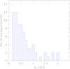 |
Fig. 6. Distribution of the uncertainties of the ⟨Bz⟩ measurements presented in this survey. |
9. The efficiency of the magnetic field measurements in WDs
In this survey we have used two different instruments, FORS2 and ISIS, and the ISIS instrument was used with two different settings, one with the red arm and one with the blue arm. The moderate-resolution spectropolarimeter ISIS is a rather different instrument than FORS2 in two important ways. First, all of the Balmer lines in the visible window, including Hα can be observed simultaneously. Secondly, the spectral resolving power in the blue arm is about 2500, almost twice the value (R ≈ 1400) used in FORS2 in the same region, and about 8600 in the red arm. Measurements using two arms may be made simultaneously, and therefore combined to improve the measurement precision. In this section we make a comparison of the efficiency of the results obtained adopting different instruments and instrument settings, by analysing separately the results obtained with FORS2, with the blue arm and with the red arm of the ISIS instrument, and we also comment on the efficiency of the field measurements as a function of stellar temperature. In our forthcoming papers, this analysis will be continued by incorporating new magnetic field data obtained with the ESPaDOnS instrument of the CFHT and with the grism 1200R of the FORS2 instrument.
9.1. The efficiency of the instruments as photon counters
The most basic comparison is to check the efficiency of the different spectropolarimeters simply as photon-counters, independently of telescope size. This comparison could be carried out with the Exposure Time Calculators of the respective instruments, but the data obtained from our survey allow us to make a more realistic comparison that takes into account also the polarimetric optics of the instruments. An obvious way to perform this exercise is to compare the measurements obtained on the same stars. In our survey, three targets were observed (at different epochs) with both FORS2 and the blue arm of ISIS: WD 1031−114, WD 1105−048 and WD 1327−083. Thin cirrus and clouds were present on sky during WHT observations, and during the observation of WD 1105−048 obtained on 2016-07-02 with FORS2, so this dataset cannot be used to properly measure the photon collection efficiency. However, since the magnitudes of almost all of our targets are known from previous studies with a good accuracy, it is possible to calculate the quantity (7)
(7)
where texp is the exposure time, V the star magnitude, A the telescope primary mirror area, (S/N)max the peak S/N per Å, k an average extinction coefficient in the observed spectral range, and X the airmass. By considering only the observations obtained during clear nights and with good seeing, we compared statistically the E values for the three instruments, and we found that for our target list of WDs the efficiency of FORS2 in the blue regions and that of ISIS in the blue arm are roughly similar.
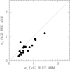 |
Fig. 7. Uncertainties of the observations obtained simultaneously in the red arm and in the blue arm of ISIS. The single star above the equality line is a DB star with only a rather weak line at 6678 Å and a low ratio red/blue flux because of Teff ∼ 25 000 K. All the remaining points refer to DA WDs. |
9.2. Comparison of the precision of the field measurements obtained with the two arms of the ISIS instrument, and with the FORS2 instrument
The uncertainty of field measurements decreases with the number of the observed spectral lines, their strength and slope, and their wavelength (the Zeeman π − σ splitting is proportional to λ 2). In the case of our ISIS observations of DA WDs, the spectral range observed in the blue arm includes Balmer lines from Hβ to H9, while the red arm includes Hα only. Roughly speaking, in terms of measurement precision, the fact that Hα is at longer wavelength than the remaining Balmer lines does not fully balance the fact that the blue arm includes up to six times more Balmer lines than the red arm (as (6500/4400)2 ∼ 2.1). Furthermore, for equal exposure time, a higher S/N is reached in the blue arm than in the red arm. On the other hand, the red arm has about three times larger spectral resolution than the blue arm. Figure 7 shows the uncertainties of the fields measurements obtained in the red and in the blue arm for DA WDs (observations in the two arms were obtained simultaneously with the use of the dichroic).
Another way to analyse the efficiencies of the field measurements is by plotting error bars agains the S/N for the various instrument modes and setting, as is done in Fig. 8.
It appears that the relationship between the uncertainty σ⟨Bz⟩ of the ⟨Bz⟩ measurements and the S/N per Å as obtained with the blue arm of ISIS is very similar to the relationship that describes the FORS2 data. Thus for blue arm field measurements, the standard errors are about twice as large using ISIS as using FORS2 for the same shutter time. In contrast, the red arm provides uncertainties that range from roughly 25% smaller than those from the blue arm to almost two times smaller, even though the S/N per Å is always smaller in the red arm measurement than in the blue arm data (with the exceptions of the observations obtained in the red arm with the low resolution grating R158R). In spite of lower continuum S/N, the red arm provides substantially more accurate measurements than the blue. This is partly because of the larger Zeeman splitting at Hα compared to the higher Balmer lines (the splitting varies as λ 2), but mainly because the higher resolving power allows us to exploit the large slope and polarisation signal near the deep and sharp core of Hα to obtain a more tightly constrained slope in the correlation diagram. In the future we will investigate whether the use of grism 1200R (and R ≈ 2800) with FORS2 would bring to a higher sensitivity in our measurements.
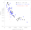 |
Fig. 8. Uncertainties versus S/N per Å for the field measurements obtained with the FORS2 instrument (black solid squares), and with the ISIS instrument in the blue arm (blue filled circles) and in the red arm (red empty circles). |
9.3. Efficiency of the field measurements as a function of spectral type
It was pointed out in Sect. 9.2 that the precision of field measurements depends on the specific features of spectral lines. These in turn depend on stellar temperature. In general we can expect that in two DA WDs of similar magnitude but different temperature, field measurements will be more precise in cooler than in hotter stars, because cooler WDs have deeper and steeper Balmer lines, at least down to Teff ≈ 7000 K. To express this concept in a more quantitative way, we may consider the product S/N × σ⟨Bz⟩ as a function of the spectral type (or stellar temperature) as a proxy for the efficiency of the field measurement. In order to get figures close to unity, it is convenient to divide the S/N by 1000, and expresss σ⟨Bz⟩ in kG. Figure 9 shows the product of the errorbar σ⟨Bz⟩ and the peak S/N per Å versus the effective temperature of all DA WDs observed in this survey. This plot tells us for instance that a field measurements obtained in the blue arm of the ISIS instrument with a S/N per Å = 1000 in a DA1.0 WD has a 1 kG uncertainty. A measurement with same peak S/N on a DA4.0 WD would have an uncertainty of about 0.3 kG. More generally, measurements with the same peak S/N in DA1.0 stars have error bars 3–4 four times higher than in the coolest WDs. From the practical point of view, one should also remember that cooler WDs are fainter than hotter stars; therefore, in terms of shutter time the comparison may be more favourable to hotter stars.
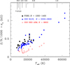 |
Fig. 9. Efficiency of the field measurements versus spectral classes for DA WDs. Spectral class (shown at the top of the diagram) is linked to the stellar temperature through the relation class = 50 400/Teff. The meaning of the symbols is the same as in Fig. 8. |
9.4. Precision versus exposure time
During observation planning it is clearly useful to have an idea of the precision than may be achieved as a function of exposure time. While it is easy to anticipate that σ⟨Bz⟩ ∝ t−1/2, it is less obvious how to express the resulting precision in real field strength units. Figure 10, combined with the use of the instrument Exposure Time Calculator, helps to associate the precision that may be achived as a function of exposure time. Clearly, the final numbers depend on the WD spectral class, but as a first approximation one can see that in order to reach a precision of 3–400 G, one has to reach a S/N of 1000, but that with half the exposure time needed to reach a S/N = 1000 per Å one can still obtain an uncertainty better than 0.5 kG, while to go below 0.2 kG one needs a four times longer exposure time.
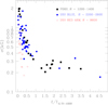 |
Fig. 10. Uncertainty reached as a function of the exposure time for the field measured obtained with the FORS2 instrument (black solid circles), and with the ISIS instrument in the red and in the blue arm (blue filled circles and red empty circles, respectively). Exposure time is normalised to the time needed to obtained S/N = 1000 per Å. The meaning of the symbols is the same as in Figs. 8 and 9. |
10. Discussion
In our surveys we had two main science objectives.
-
(1)
Increasing substantially the number of WDs that have been searched for kG-level longitudinal magnetic fields, in order to clarify the frequency of occurrence of the weakest detectable fields in various types of WDs. A basic goal was to determine whether fields occur at the ⟨Bz⟩ ∼ 1 kG level (frequently, sometimes, never), and particularly to discover whether we have reached a lower limit of the field distribution yet.
-
(2)
Improve the monitoring of the (currently small) number of MWDs of any type known to have kG-level fields, in order to develop our modelling techniques and obtain models of as many such stars as possible.
All ISIS spectropolarimetry, except for one star (40 Eri B, see Sect. 10.3.2) were obtained only for survey purpose, and not to monitor any individual star.
In this section we discuss separately the survey component of the FORS2 observing runs (Sect. 10.1), the ISIS survey (Sect. 10.2), and the monitoring of individual stars (Sect. 10.3). Finally, we discuss some preliminary statistical conclusions (Sect. 10.4).
10.1. FORS2 spectropolarimetric survey
Of the ten newly observed FORS2 stars, two observations failed because of incorrect wave-plate settings, and one of the stars, WD 1917−077, was found to be effectively a DC star (it is classified as a DBQA5, but all absorption features are broad and shallow, so no field measurement was attempted).
Of the seven remaining survey stars observed with FORS2, six are DA white dwarfs with V magnitudes in range of 11.4–13.1, while one is a fainter DZ star. All have been previously observed for magnetic fields, but with higher field detection thresholds. All have been studied using low-resolution optical spectra (e.g. Gianninas et al. 2011). In such data, fields of about ⟨|B|⟩ > 1 MG are readily visible, so normal parameter fitting identifies and filters for such fields. Furthermore, the DA stars have been observed with high-resolution optical spectroscopy, (mostly in the context of the SPY project, e.g. Koester et al. 2009), providing upper limits on ⟨|B|⟩ of roughly 50 kG.
For all DA WDs, the computed value of σ⟨Bz⟩ is between 220 and 310 G. Only one DA star appears to show a marginal detection: WD 1031−114, with ⟨Bz⟩ = −870 ± 290 G. This detection is significant at just barely 3 σ⟨Bz⟩. The single DZ star, WD 2138−332, also shows a marginally significant field detection, at the 3.3 σ⟨Bz⟩ level. These two stars are discussed individually below.
Our uncertainties for the DA star ⟨Bz⟩ measurements are about a factor of two smaller than those obtained for previous measurements of some of the same stars. This improvement is due to the longer integration times that we have used and the higher-resolution grism that we have adopted (1200B instead of 600B). We have reached a level of uncertainty that should reveal fields of order ⟨Bz⟩ ≈ 1−1.5 kG if they are present in any of the stars of this small sample, and it appears that we may have detected one such field.
10.2. ISIS spectropolarimetric survey
Using ISIS we made 54 ⟨Bz⟩ measurements on 38 WDs. Most of the stars observed have V magnitudes between 12.5 and 14. Using total shutter times of somewhat more than one hour, the data have uncertainties σ⟨Bz⟩ below 300 G for one observation of each of 11 stars; for the remainder, σ⟨Bz⟩ is mostly in the range between 300 and 700 G. It appears that the high measurement efficiency of ISIS in the red arm is a sufficiently important factor to compensate for the relative mirror area of about 4:1 in favour of FORS2; the two spectropolarimeters provide data with roughly similar uncertainties for observations with similar shutter times on stars with similar magnitude. A larger ⟨Bz⟩ survey of DA and related WDs with ISIS would also be capable of revealing fields of about 1 kG in a statistically interesting sample of some tens of WDs.
Of the 36 WDs for which useful ⟨Bz⟩ measurements were obtained with ISIS (two stars had featurless spectra), all had been previosuly studied at low resolution, and were known to be non-magnetic at the 1 MG or higher level. About 40% have been observed at high resolution in unpolarised light, and thus probably do not have fields exceeding ⟨|B|⟩ ∼ 50 kG. Three stars observed with ISIS (WD 1031−114, WD 1105−048, WD 1327−083) have also been observed with FORS2. WD 1105−048 is strongly suspected of hosting a variable field near the detection threshhold, and will be discussed in Sect. 10.3. For the other two stars, measurements with the two instruments provide concordant non-detections.
As discussed above, the values of σ⟨Bz⟩ for the ISIS ⟨Bz⟩ measurements mostly lie in the range of 180–700 G, and are thus sensitive to fields larger than roughly 1–2 kG. One new MWD was discovered in this sample: WD 2047+372 (Landstreet et al. 2016). This WD has a constant field modulus of ⟨|B|⟩ ≈ 60 kG, and a longitudinal field which varies between −12 and +15 kG with a period of 0.243 d (Landstreet et al. 2017). No other stars of the ISIS survey sample have significant fields. This discovery increased the number of confirmed MWDs having fields below 200 kG from six to seven (see Table 6 of Landstreet et al. 2017). Even a single discovery is capable of having a substantial effect on the statistics of weak-field frequency.
10.3. Comments on individual stars
10.3.1. WD 2359−434
With FORS2, we have obtained four new ⟨Bz⟩ measurements of the known MWD WD 2359−434 (Koester et al. 1998; Aznar Cuadrado et al. 2004). These data have already been reported by us in a previous paper (Landstreet et al. 2017), and were analysed together with a large data set obtained with ESPaDOnS on the CFHT. The full data set reveal a field whose ⟨Bz⟩ values always lie between roughly 0 and 10 kG, while the field modulus varies between about 50 and 100 kG. These data have been used in the modelling of the strongly non-dipolar magnetic field geometry of this star (Landstreet et al. 2017).
10.3.2. 40 Eri B = WD 0413−077
This star has been monitored both with ISIS and with the ESPaDOnS instrument (Landstreet et al. 2015) to attempt to confirm the magnetic field of ⟨Bz⟩ ∼ 4 kG reported by Fabrika et al. (2003). Landstreet et al. (2015) did not find any evidence of the presence of a magnetic field above the level of about 250 G. In this survey we also report previously unpublished measurements obtained using the red arm of the ISIS instrument with the low resolution grating R158R. All are consistent with no field detection.
10.3.3. WD 0446−789
This star was originally discovered to be a MWD with FORS1 by Aznar Cuadrado et al. (2004). Two of their non-zero ⟨Bz⟩ measurements hinted at possible variability. Our four new data points, while all having the same sign as the discovery observations, further confirm at higher precision the probability that the star is a magnetic variable. The data are not numerous enough to strongly constrain the star’s period, but if we assume that the ⟨Bz⟩ variations are roughly sinusoidal in form, then the longest period consistent with the ⟨Bz⟩ data is about 10 d, the mean field B0 is between −5500 and −4000 G, and the amplitude of the ⟨Bz⟩ curve is ∼1400 − 2400 G.
The line core of Hα is not broadened enough to provide a very strong constraint on ⟨|B|⟩, apart from establishing 20 − 25 kG as an upper limit (see Landstreet et al. 2012, Fig. 3)
Combining all these constraints, it appears possible that that the global field of WD 0446−789 may be roughly dipolar, with a polar field of the order of 30 kG. If this model is basically correct, both the angle between the line of sight and the stellar rotation axis, and the angle between the rotation and magnetic axes, are small, with one of order 20° − 30°, and the other of the order of 5°–10°.
10.3.4. WD 1031−114
Our survey data from FORS2 and ISIS reported in this paper has identified as a possible very weak field MWD the DA1.9 star WD 1031−114. One of our FORS2 measurement was ⟨Bz⟩ = −870 ± 290 G, barely significant at the 3 σ level, while another ISIS measurement (with uncertainty more than three times larger than the measurement obtained with FORS2) did not show a significant field. This star is not yet confirmed as magnetic, but is well worth following up with further measurements achieving uncertainties of the order of 300 G or better. Assuming a roughly dipolar configuration for the magentic field, our positive field detection also places a constraint on the mean field modulus ⟨|B|⟩, namely ⟨|B|⟩ ≳ 3 kG. Zeeman broadening or splitting of the Stokes I profile of Hα may be detected only if ⟨|B|⟩ ≳ 25 kG, i.e., several times larger than the lower limit of 3 kG.
10.3.5. WD 1105−048
WD 1105−048 has a possible magnetic field detected as ⟨Bz⟩ = 3340 ± 655 G, significant at the 5 σ level, in one of two previously published field measurements with FORS1; the other measurement of about the same precision showed no significant field (Aznar Cuadrado et al. 2004; Landstreet et al. 2012). A barely significant detection of a –8 kG field was also reported by Valyavin et al. (2006). On the basis of this evidence we have considered WD 1105−048 to be probable but unconfirmed MWD. We have obtained three new FORS2 field measurements and one new ISIS observation. Two of the FORS2 measurements have uncertainties of ∼270 G; the other two measurements have substantially larger uncertainties. One of the two new high-precision FORS2 measurements shows a field of ⟨Bz⟩ = 2145 ± 270 G, significant at the 7.9 σ level. The other three measurements are all consistent with zero field. However, with now two high-significance field detections of this star, we now consider WD 1105−048 to be a confirmed MWD.
The field of the star appears to vary between a ⟨Bz⟩ value of roughly zero and about +3 kG in such a way that ⟨Bz⟩ is usually closer to the minimum than to the maximum value. This suggests a field ⟨|B|⟩ of the order of 10 kG or larger. The intensity profile of Hα does not show any obvious broadening of the non-LTE line core (Landstreet et al. 2012, Fig. 3), suggesting that ⟨|B|⟩ is less than about 20–25 kG.
10.3.6. WD 2047−372
Our single ISIS field measurement of WD 2047+372 showed a non-zero field of ⟨Bz⟩ = 100 ± 410 G, a marginally significant value, but confirmed the presence of a field through an almost resolved Zeeman triplet in Hα. This star was then observed extensively with ESPaDOnS, revealing a longitudinal field ⟨Bz⟩ varying sinusoidally between −12 and +15 kG, and a ⟨|B|⟩ value that is virtually constant at 60 kG. The resulting data set has been described and modelled with a simple dipolar field structure (Landstreet et al. 2017).
10.3.7. WD 2105−820
This star was previously suggested as possibly magnetic by Koester et al. (1998), who estimated that a field of ⟨|B|⟩ ≈ 42 kG might be present. Landstreet et al. (2012) obtaind five spectropolarimetric observations from FORS2, which showed a longitudinal field ranging in ⟨Bz⟩ values from +8.2 to +11.4 G, fully confirming the presence of a magnetic field. This range is about as large as would be expected if ⟨Bz⟩ were actually constant at +9500 G. We have three new FORS2 measurements of this WD, all with ⟨Bz⟩ values that are positive but smaller than the five previous measurements. One of the measurements, of ⟨Bz⟩ = 3545 ± 685 G, is different enough from the earlier data to establish with high probability that the field of this star is in fact mildly variable. It is clear from the precision of these measurements that a FORS2 time series with the attainable precision would probably reveal a weakly variable field from which the rotation period could be derived. However, the data are sufficiently widely spaced to provide no useful constraints on the rotation period.
A single measurement of ⟨Bz⟩ = +5.3 ± 0.3 kG was obtained by Farihi et al. (2018). This measurement confirms the presence of a field in this star, but because this measurement was made using only Hα, in contrast to our measurements using only higher Balmer lines, it is unlikely that this measurement is on exactly the same scale as ours.
Landstreet et al. (2012) modelled the star’s magnetic field as a simple dipole having either the magnetic axis nearly aligned with the rotation axis, or a viewing geometry in which the star is viewed with the rotation axis nearly aligned with the line of sight. The new data do not discredit this model, but suggest that the inclination of the rotation axis to the line of sight is slightly larger than previously estimated, or that the angle between the rotation axis and the dipole axis is slightly larger than estimated. However, the smaller of these two angles is still probably less than about 20°.
10.3.8. WD 2138−332
Our single observation of the DZ star WD 2138−332 yields a field of ⟨Bz⟩ = 3300 ± 990 G, significant at the 3.3σ level. The larger value of σ⟨Bz⟩ compared to the DA stars is due to a combination of fainter magnitude, shorter integration time, and the weakness of the Mg I, Ca I and II, and Fe I lines used to measure the field. This single detection is not significant enough for us to consider that this star definitely has a weak magnetic field, but it certainly calls for further observations, which have been proposed. Low S/N spectra of the DZ star WD 2138−332 taken with FEROS and obtained from the ESO Archive show deep and sharp metal lines. Modelling of these lines would probably allow one to set upper limits on ⟨|B|⟩ of the order of 20 kG. A field upper limit of this level would be consistent with the marginal detection of non-zero ⟨Bz⟩, but does nothing to support the possible field detection. Note that this star is within the sphere of radius 20 pc centred on the Sun.
10.4. Preliminary statistical considerations
The surveys of Aznar Cuadrado et al. (2004), Jordan et al. (2007) and Landstreet et al. (2012) looked in total at 30 stars for which no previous study had pointed to a magnetic field of any strength, plus two stars (WD 2105−820 and WD 2359−434) for which Koester et al. (1998) had already suggested the presence of weak fields, both of which were confirmed by spectropolarimetry to be MWDs. Among the remaining 30 stars, two new very weak field stars were found (WD 0446−789 and WD 1105−048). This suggests a frequency among what is essentially a magnitude limited survey of about 6 ± 4% for fields in the range of 1 ≤ ⟨Bz⟩ ≤ 10 kG.
We have surveyed 14 WDs with measurements obtaining σ⟨Bz⟩ ≤ 300 G and a total of 20 with σ⟨Bz⟩ ≤ 500 G. Both these samples contain the one suspected magnetic star (WD 1031−114), for which the largest measured ⟨Bz⟩ value is actually slightly below 1 kG. Considering this star to be really magnetic, with a ⟨Bz⟩ values in the 1–10 kG range, we have a frequency of occurence of fields in this range of roughly 5 ± 5%, in reasonable agreement with the older result. These two frequency estimates both have rather large relative uncetainties, but both suggest that very weak WD fields occur, in the range of 1 ≤ ⟨Bz⟩ ≤ 10 kG, roughly as frequently as larger fields, which appear to have a frequency of occurence of the order of 3 − 4% per dex (per factor of ten in field strength) as found for example by Kawka et al. (2007).
To summarise, our data do not suggest that we have reached a minimum field strength at ⟨Bz⟩ ∼ 1 kG below which WD fields become extremely rare, nor have we reached a field strength at this level at which WD fields become ubiquitous. Instead, the situation prevailing for stronger field MWDs, that fields are uncommon but not rare, seems to continue.
We shall postpone a more detailed discussion of the statistics of detection of very weak fields to the next paper in this series, which will add to the data here the results of a parallel survey using ESPaDOnS at the CFHT, and examine these data in a larger context.
11. Conclusions
We have reported several significant results, both of instrumental nature and concerning the observation of very weak magnetic fields in WDs.
11.1. Instrumental advances
We have shown that with the ESO’s FORS2 instrument in spectropolarimetric mode it is practical to measure the mean longitudinal field with uncertainties of the order of 250–300 G in DA and DB stars having V ≲ 13.
Similarly, we have established that the spectropolarimeter ISIS on the WHT is an effective instrument for searching for and measuring very weak fields in WDs. First we have shown that field measurements with ISIS on known magnetic Ap/Bp stars are consistent with those obtained with other spectropolarimeters. We have further established that the use of a dichroic does not introduce spurious effect when we measure the magnetic fields, and therefore the red and blue arm of the instrument can be used simultaneously. This significantly improves the power of ISIS for measuring very weak WD fields. Like FORS2, ISIS is capable of achieving σ⟨Bz⟩ values of around 300 G on bright WDs.
We have compared the efficiency of ISIS and FORS2 in several ways, finding that, in terms of photon detection efficiency, in the blue spectral region FORS2 with grism 1200B and the blue arm of ISIS with grating R600B have a comparable efficiency (per unit of telescope collecting area). When we compare field measurements in the blue spectral region obtained with similar S/N (or photon count) per Å, the two instruments yield essentially similar field uncertainties. Thus their effectiveness as faint object, high-precision spectropolarimeters is similar, apart from the difference in efficiency and telescope aperture.
A very important asset of ISIS is that the red arm is equipped with a grating that allows one to observe with R ≈ 8600. It is found that this is an extremely valuable tool for weak field measurements of stars with a substantial Hα line. For a given S/N level, the field uncertainty derived from Hα alone is of the order of two times smaller than that obtained from using five Balmer lines in the blue window. This high detection efficiency is possible because the resolving power is high enough to almost resolve the sharp, deep non-LTE core of Hα, which substantially reduces σ⟨Bz⟩ compared to a meaurement which does not resolve this core (see the discussion in Landstreet et al. 2015). Using the red and blue arms of ISIS together, we are able to achieve roughly the same uncertainties σ⟨Bz⟩ in a given integration time as is achieved with FORS2 + grism 1200B on a telescope with four times larger area.
The conclusion is that both FORS2 and ISIS can quite practically carry out a large survey searching for fields of ⟨Bz⟩ ∼ 1 kG in the more than 150 DA stars of V ≲ 14 mag.
11.2. Astrophysical results
In the course of the FORS2 survey presented in this paper we have obtained several ⟨Bz⟩ measurements of each of four previously known MWDs: WD 0446−789, WD 2051−208, WD 2105−820, and WD 2359−434. The first three of these MWDs all have somewhat variable ⟨Bz⟩ values, and we have used the observed range of these values, together with very rough estimates of ⟨|B|⟩, to propose very approximate dipole-like field models (for WD 0446−789, see Sect. 10.3.3; for WD 2051−208 and WD 2105−820, see Landstreet et al. 2012, 2017). The FORS2 ⟨Bz⟩ data for WD 2359−434 have already been published, and have been used in the construction of a reasonably constrained field geometry model of the MWD, which quite clearly departs from a simple dipole (Landstreet et al. 2017). With the ISIS and the ESPaDOnS instruments we have also discovered and monitored the very weak-field star WD 2047+372, for which we now have enough ⟨Bz⟩ and ⟨|B|⟩ data to establish the 0.24 d rotation period and to construct a well-constrained dipole model (Landstreet et al. 2016, 2017).
Another significant result of our survey is to confirm the magnetic nature of WD 1105−048, which was previously in doubt because only one really convincing field detection had previously been achieved. This star is the MWD with the weakest confirmed magnetic field so far found. The field cleaerly varies between ⟨Bz⟩ ≈ 0 and 2100 G, with a still unknown period.
About 20 bright WDs of our sample have been surveyed with uncertainties ≲500 G, so that we are sensitive to fields of 1–2 kG. For most of the stars of our target list, we have strong upper limits on ⟨Bz⟩ of at most about 2 kG. In the course of the survey, one DA and one DZ star, WD 1031−114 and WD 2138−332, have yielded one ⟨Bz⟩ measurement each that is significantly different from zero at about the 3 σ⟨Bz⟩ level. These could be new examples of extremely weak fields like that of WD 1105−048, or they could be spurious detections. We plan to re-observe both these stars as soon as practical.
From this modest survey, it already seems clear that even at the 1 kG level, magnetic fields are still present in WDs, but not common. We have not found a floor beneath which fields die away, nor a level at which fields appear to be ubiquitous.
Acknowledgments
This survey is based on observations collected at the WHT operated on the island of La Palma by the Isaac Newton Group, programmes P28 during semester 15A and P17 during semester 15B, and at the European Organisation for Astronomical Research in the Southern Hemisphere under ESO programmes 095.C-0855 and 096.C-0159. A smaller number of observations were obtained at the ING WHT in the context of ING programme P11 during semester 13B, and at the ESO VLT as backup during programme ID 093.D-0680. This project has made extensive use of the Montreal White Dwarf Database (www.MontrealWhiteDwarfDatabase.org). Work by one of us (JDL) has been supported by the Natural Sciences and Engineering Research Council of Canada. We thank the referee Dr. Adela Kawka for very useful comments which contributed to improve the manuscript.
References
- Angel, J. R. P., & Landstreet, J. D. 1970a, ApJ, 162, L61 [NASA ADS] [CrossRef] [Google Scholar]
- Angel, J. R. P., & Landstreet, J. D. 1970b, ApJ, 160, L147 [NASA ADS] [CrossRef] [Google Scholar]
- Angel, J. R. P., & Landstreet, J. D. 1971a, ApJ, 164, L15 [NASA ADS] [CrossRef] [Google Scholar]
- Angel, J. R. P., & Landstreet, J. D. 1971b, ApJ, 165, L71 [NASA ADS] [CrossRef] [Google Scholar]
- Angel, J. R. P., & Landstreet, J. D. 1972, ApJ, 178, L21 [NASA ADS] [CrossRef] [Google Scholar]
- Angel, J. R. P., Borra, E. F., & Landstreet, J. D. 1981, ApJS, 45, 457 [NASA ADS] [CrossRef] [Google Scholar]
- Angel, J. R. P., Liebert, J., & Stockman, H. S. 1985, ApJ, 292, 260 [NASA ADS] [CrossRef] [Google Scholar]
- Appenzeller, I. 1967, PASP, 79, 136 [NASA ADS] [CrossRef] [Google Scholar]
- Appenzeller, I., & Rupprecht, G. 1992, The Messenger, 67, 18 [NASA ADS] [Google Scholar]
- Appenzeller, I., Fricke, K., Fürtig, W., et al. 1998, The Messenger, 94, 1 [NASA ADS] [Google Scholar]
- Aznar Cuadrado, R., Jordan, S., Napiwotzki, R., et al. 2004, A&A, 423, 1081 [NASA ADS] [CrossRef] [EDP Sciences] [Google Scholar]
- Bagnulo, S., & Landstreet, J. D. 2015, Stellar Magnetic Fields, eds. L. Kolokolova,J. Hough, & A.-C. Levasseur-Regourd, 224 [Google Scholar]
- Bagnulo, S., Landi Degl’Innocenti, M., Landolfi, M., & Mathys, G. 2002a, A&A, 394, 1023 [NASA ADS] [CrossRef] [EDP Sciences] [Google Scholar]
- Bagnulo, S., Szeifert, T., Wade, G. A., Landstreet, J. D., & Mathys, G. 2002b, A&A, 389, 191 [NASA ADS] [CrossRef] [EDP Sciences] [Google Scholar]
- Bagnulo, S., Landolfi, M., Landstreet, J. D., et al. 2009, PASP, 121, 993 [NASA ADS] [CrossRef] [Google Scholar]
- Bagnulo, S., Landstreet, J. D., Fossati, L., & Kochukhov, O. 2012, A&A, 538, A129 [NASA ADS] [CrossRef] [EDP Sciences] [Google Scholar]
- Bagnulo, S., Fossati, L., Kochukhov, O., & Landstreet, J. D. 2013, A&A, 559, A103 [NASA ADS] [CrossRef] [EDP Sciences] [Google Scholar]
- Bagnulo, S., Cox, N. L. J., Cikota, A., et al. 2017a, A&A, 608, A146 [NASA ADS] [CrossRef] [EDP Sciences] [Google Scholar]
- Bagnulo, S., Nazé, Y., Howarth, I. D., et al. 2017b, A&A, 601, A136 [NASA ADS] [CrossRef] [EDP Sciences] [Google Scholar]
- Bohlin, R. C. 1995, in Calibrating Hubble Space Telescope. Post Servicing Mission, eds. A. P. Koratkar, & C. Leitherer, 49 [Google Scholar]
- Borra, E. F., & Landstreet, J. D. 1978, ApJ, 222, 226 [NASA ADS] [CrossRef] [Google Scholar]
- Bychkov, V. D., Bychkova, L. V., & Madej, J. 2016, MNRAS, 455, 2567 [NASA ADS] [CrossRef] [Google Scholar]
- Donati, J.-F., & Landstreet, J. D. 2009, ARA&A, 47, 333 [NASA ADS] [CrossRef] [MathSciNet] [Google Scholar]
- Eggen, O. J., & Greenstein, J. L. 1965, ApJ, 141, 83 [NASA ADS] [CrossRef] [Google Scholar]
- Eggen, O. J., & Greenstein, J. L. 1967, ApJ, 150, 927 [NASA ADS] [CrossRef] [Google Scholar]
- Euchner, F., Jordan, S., Beuermann, K., Gänsicke, B. T., & Hessman, F. V. 2002, A&A, 390, 633 [NASA ADS] [CrossRef] [EDP Sciences] [Google Scholar]
- Euchner, F., Jordan, S., Beuermann, K., Reinsch, K., & Gänsicke, B. T. 2006, A&A, 451, 671 [NASA ADS] [CrossRef] [EDP Sciences] [Google Scholar]
- Fabrika, S. N., Valyavin, G. G., & Burlakova, T. E. 2003, Astron. Lett., 29, 737 [NASA ADS] [CrossRef] [Google Scholar]
- Farihi, J., Dufour, P., Napiwotzki, R., & Koester, D. 2011, MNRAS, 413, 2559 [NASA ADS] [CrossRef] [Google Scholar]
- Farihi, J., Fossati, L., Wheatley, P. J., et al. 2018, MNRAS, 474, 947 [NASA ADS] [CrossRef] [Google Scholar]
- Ferrario, L., de Martino, D., & Gänsicke, B. T. 2015, Space Sci. Rev., 191, 111 [NASA ADS] [CrossRef] [Google Scholar]
- Gaia Collaboration(Brown, A. G. A., et al.) 2018, A&A, 616, A1 [NASA ADS] [CrossRef] [EDP Sciences] [Google Scholar]
- Gianninas, A., Bergeron, P., & Ruiz, M. T. 2011, ApJ, 743, 138 [NASA ADS] [CrossRef] [Google Scholar]
- Greenstein, J. L., Gunn, J. E., & Kristian, J. 1971, ApJ, 169, L63 [NASA ADS] [CrossRef] [Google Scholar]
- Hamuy, M., Walker, A. R., Suntzeff, N. B., et al. 1992, PASP, 104, 533 [NASA ADS] [CrossRef] [Google Scholar]
- Hill, G. M., Bohlender, D. A., Landstreet, J. D., et al. 1998, MNRAS, 297, 236 [NASA ADS] [CrossRef] [Google Scholar]
- Holberg, J. B., Barstow, M. A., & Green, E. M. 1997, ApJ, 474, L127 [NASA ADS] [CrossRef] [Google Scholar]
- Holberg, J. B., Oswalt, T. D., & Sion, E. M. 2002, ApJ, 571, 512 [NASA ADS] [CrossRef] [Google Scholar]
- Holberg, J. B., Bergeron, P., & Gianninas, A. 2008, AJ, 135, 1239 [NASA ADS] [CrossRef] [Google Scholar]
- Holberg, J. B., Oswalt, T. D., Sion, E. M., & McCook, G. P. 2016, MNRAS, 462, 2295 [NASA ADS] [CrossRef] [Google Scholar]
- Hollands, M. A., Gänsicke, B. T., & Koester, D. 2015, MNRAS, 450, 681 [NASA ADS] [CrossRef] [Google Scholar]
- Hubrig, S., North, P., Schöller, M., & Mathys, G. 2006, Astron. Nachr., 327, 289 [NASA ADS] [CrossRef] [Google Scholar]
- Ilyin, I. 2012, Astron. Nachr., 333, 213 [NASA ADS] [CrossRef] [Google Scholar]
- Jordan, S. 1992, A&A, 265, 570 [NASA ADS] [Google Scholar]
- Jordan, S., Aznar Cuadrado, R., Napiwotzki, R., Schmid, H. M., & Solanki, S. K. 2007, A&A, 462, 1097 [NASA ADS] [CrossRef] [EDP Sciences] [Google Scholar]
- Kawka, A., & Vennes, S. 2012, MNRAS, 425, 1394 [NASA ADS] [CrossRef] [Google Scholar]
- Kawka, A., & Vennes, S. 2014, MNRAS, 439, L90 [NASA ADS] [CrossRef] [Google Scholar]
- Kawka, A., Vennes, S., Schmidt, G. D., Wickramasinghe, D. T., & Koch, R. 2007, ApJ, 654, 499 [NASA ADS] [CrossRef] [Google Scholar]
- Kemic, S. B. 1974, ApJ, 193, 213 [NASA ADS] [CrossRef] [Google Scholar]
- Kemp, J. C. 1970, ApJ, 162, L69 [NASA ADS] [CrossRef] [Google Scholar]
- Kemp, J. C., Swedlund, J. B., Landstreet, J. D., & Angel, J. R. P. 1970, ApJ, 161, L77 [NASA ADS] [CrossRef] [Google Scholar]
- Kepler, S. O., Pelisoli, I., Jordan, S., et al. 2013, MNRAS, 429, 2934 [NASA ADS] [CrossRef] [Google Scholar]
- Kepler, S. O., Pelisoli, I., Koester, D., et al. 2015, MNRAS, 446, 4078 [NASA ADS] [CrossRef] [Google Scholar]
- Kepler, S. O., Pelisoli, I., Koester, D., et al. 2016, MNRAS, 455, 3413 [NASA ADS] [CrossRef] [Google Scholar]
- King, D. L. 1985, La Palma Technical Note, 31 [Google Scholar]
- Kleinman, S. J., Kepler, S. O., Koester, D., et al. 2013, ApJS, 204, 5 [NASA ADS] [CrossRef] [MathSciNet] [Google Scholar]
- Koester, D., Dreizler, S., Weidemann, V., & Allard, N. F. 1998, A&A, 338, 612 [NASA ADS] [Google Scholar]
- Koester, D., Napiwotzki, R., Christlieb, N., et al. 2001, A&A, 378, 556 [NASA ADS] [CrossRef] [EDP Sciences] [Google Scholar]
- Koester, D., Rollenhagen, K., Napiwotzki, R., et al. 2005, A&A, 432, 1025 [NASA ADS] [CrossRef] [EDP Sciences] [Google Scholar]
- Koester, D., Voss, B., Napiwotzki, R., et al. 2009, A&A, 505, 441 [NASA ADS] [CrossRef] [EDP Sciences] [Google Scholar]
- Külebi, B., Jordan, S., Euchner, F., Gänsicke, B. T., & Hirsch, H. 2009, A&A, 506, 1341 [NASA ADS] [CrossRef] [EDP Sciences] [Google Scholar]
- Landstreet, J. D. 1982, ApJ, 258, 639 [NASA ADS] [CrossRef] [Google Scholar]
- Landstreet, J. D. 1992, A&ARv, 4, 35 [NASA ADS] [CrossRef] [Google Scholar]
- Landstreet, J. D., & Angel, J. R. P. 1971, ApJ, 165, L67 [NASA ADS] [CrossRef] [Google Scholar]
- Landstreet, J. D., & Mathys, G. 2000, A&A, 359, 213 [NASA ADS] [Google Scholar]
- Landstreet, J. D., Bagnulo, S., Fossati, L., Jordan, S., & O’Toole, S. J. 2012, A&A, 541, A100 [NASA ADS] [CrossRef] [EDP Sciences] [Google Scholar]
- Landstreet, J. D., Bagnulo, S., & Fossati, L. 2014, A&A, 572, A113 [NASA ADS] [CrossRef] [EDP Sciences] [Google Scholar]
- Landstreet, J. D., Bagnulo, S., Valyavin, G. G., et al. 2015, A&A, 580, A120 [NASA ADS] [CrossRef] [EDP Sciences] [Google Scholar]
- Landstreet, J. D., Bagnulo, S., Martin, A., & Valyavin, G. 2016, A&A, 591, A80 [NASA ADS] [CrossRef] [EDP Sciences] [Google Scholar]
- Landstreet, J. D., Bagnulo, S., Valyavin, G., & Valeev, A. F. 2017, A&A, 607, A92 [NASA ADS] [CrossRef] [EDP Sciences] [Google Scholar]
- Leckrone, D. S. 1974, ApJ, 190, 319 [NASA ADS] [CrossRef] [Google Scholar]
- Liebert, J., & Sion, E. M. 1979, Astrophys. Lett., 20, 53 [NASA ADS] [Google Scholar]
- Liebert, J., Angel, J. R. P., & Landstreet, J. D. 1975, ApJ, 202, L139 [NASA ADS] [CrossRef] [Google Scholar]
- Liebert, J., Angel, J. R. P., Stockman, H. S., Spinrad, H., & Beaver, E. A. 1977, ApJ, 214, 457 [NASA ADS] [CrossRef] [Google Scholar]
- Liebert, J., Bergeron, P., & Holberg, J. B. 2003, AJ, 125, 348 [NASA ADS] [CrossRef] [Google Scholar]
- Massey, P., & Gronwall, C. 1990, ApJ, 358, 344 [NASA ADS] [CrossRef] [Google Scholar]
- Massey, P., Strobel, K., Barnes, J. V., & Anderson, E. 1988, ApJ, 328, 315 [NASA ADS] [CrossRef] [Google Scholar]
- Mathys, G. 1989, A&AS, 81, 237 [NASA ADS] [Google Scholar]
- Maund, J. R. 2008, A&A, 481, 913 [NASA ADS] [CrossRef] [EDP Sciences] [Google Scholar]
- McCook, G. P., & Sion, E. M. 1987, ApJS, 65, 603 [NASA ADS] [CrossRef] [Google Scholar]
- Moehler, S., Modigliani, A., Freudling, W., et al. 2014, A&A, 568, A9 [NASA ADS] [CrossRef] [EDP Sciences] [Google Scholar]
- North, P., & Adelman, S. J. 1995, A&AS, 111, 41 [NASA ADS] [Google Scholar]
- Oke, J. B. 1990, AJ, 99, 1621 [NASA ADS] [CrossRef] [Google Scholar]
- Patat, F., Moehler, S., O’Brien, K., et al. 2011, A&A, 527, A91 [NASA ADS] [CrossRef] [EDP Sciences] [Google Scholar]
- Preston, G. W. 1970, ApJ, 160, L143 [NASA ADS] [CrossRef] [Google Scholar]
- Putney, A. 1997, ApJS, 112, 527 [NASA ADS] [CrossRef] [Google Scholar]
- Saffer, R. A., Liebert, J., & Olszewski, E. W. 1988, ApJ, 334, 947 [NASA ADS] [CrossRef] [Google Scholar]
- Scarrott, S. M., Warren-Smith, R. F., Pallister, W. S., Axon, D. J., & Bingham, R. G. 1983, MNRAS, 204, 1163 [NASA ADS] [CrossRef] [Google Scholar]
- Schmidt, G. D., & Smith, P. S. 1995, ApJ, 448, 305 [NASA ADS] [CrossRef] [Google Scholar]
- Schmidt, G. D., Harris, H. C., Liebert, J., et al. 2003, ApJ, 595, 1101 [NASA ADS] [CrossRef] [Google Scholar]
- Valyavin, G., Bagnulo, S., Fabrika, S., et al. 2006, ApJ, 648, 559 [NASA ADS] [CrossRef] [Google Scholar]
- Vornanen, T., Berdyugina, S. V., Berdyugin, A. V., & Piirola, V. 2010, ApJ, 720, L52 [NASA ADS] [CrossRef] [Google Scholar]
- Vornanen, T., Berdyugina, S. V., & Berdyugin, A. 2013, A&A, 557, A38 [NASA ADS] [CrossRef] [EDP Sciences] [Google Scholar]
- Wunner, G., Roesner, W., Herold, H., & Ruder, H. 1985, A&A, 149, 102 [NASA ADS] [Google Scholar]
- Xu, S., Jura, M., Koester, D., Klein, B., & Zuckerman, B. 2014, ApJ, 783, 79 [NASA ADS] [CrossRef] [Google Scholar]
- Zuckerman, B., Koester, D., Reid, I. N., & Hünsch, M. 2003, ApJ, 596, 477 [NASA ADS] [CrossRef] [Google Scholar]
- Zuckerman, B., Koester, D., Dufour, P., et al. 2011, ApJ, 739, 101 [NASA ADS] [CrossRef] [Google Scholar]
Appendix A:
Additional material
Log of the observations of well known magnetic Ap/Bp stars obtained with ISIS of the WHT.
Observations obtained with the retarder waveplate at position angles 0° and 90°.
Observing log.
continued.
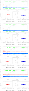 |
Fig. A.1. Stokes I, V/I and null spectra of the observed white dwarfs, and linear interpolations as explained in Sect. 6. |
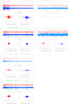 |
Fig. A.1. continued. |
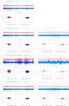 |
Fig. A.1. continued. |
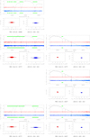 |
Fig. A.1. continued. |
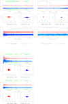 |
Fig. A.1. continued. |
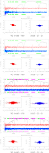 |
Fig. A.1. continued. |
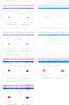 |
Fig. A.1. continued. |
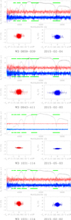 |
Fig. A.1. continued. |
 |
Fig. A.1. continued. |
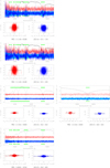 |
Fig. A.1. continued. |
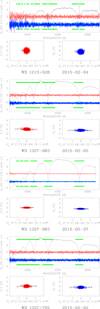 |
Fig. A.1. continued. |
 |
Fig. A.1. continued. |
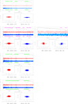 |
Fig. A.1. continued. |
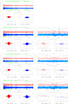 |
Fig. A.1. continued. |
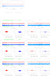 |
Fig. A.1. continued. |
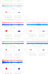 |
Fig. A.1. continued. |
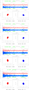 |
Fig. A.1. continued. |
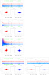 |
Fig. A.1. continued. |
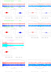 |
Fig. A.1. continued. |
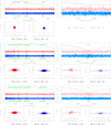 |
Fig. A.1. continued. |
All Tables
Log of the observations of well known magnetic Ap/Bp stars obtained with ISIS of the WHT.
Observations obtained with the retarder waveplate at position angles 0° and 90°.
All Figures
|
Fig. 1. Raw image of spectropolarimetric data obtained with FORS2 (top panel), ISIS blue CCD (bottom left panel) and ISIS red CCD (bottom right panel). For all images, the dynamic range is set to show the sky background, which is at the level of a few hundred ADUs (while the spectra are at the level of several thousand ADUs). The FORS2 image refers to WD 2039−202 observed on 2015-06-02. The ISIS image refers to WD 2111+498 observed on 2015-08-30. For display purpose, the images of the ISIS spectra have been trimmed in the dispersion direction. Note in ISIS images the four strips illuminated by sky background. |
| In the text | |
|
Fig. 2. Hβ (left panel) and Hα (right panel) lines of star WD 1840−111 observed with ISIS in the blue and red arm, respectively. Top panel: I profile (in arbitrary units). Second panel from top: V/I profile. Third panel from top: x = −Cz λ2(1/I)dI/dλ vs. wavelength. The green vertical lines show the wavelength intervals in which the x values clearly depart from zero, and which have been choosen to apply the least-square technique. Bottom panel: relation between V/I and x for the points within the solid green lines in the upper panels. Note that the x and V/I ranges of the Hβ plots are half the size of the corresponing ranges in the Hα plots. |
| In the text | |
|
Fig. 3. Comparison of our ISIS measurements of reference star 53 Cam = HD 65339 with the sinusoidal curve obtained by Hill et al. (1998). Filled circles refer to measurements obtained from metal lines, and empty squares to field measurements from H Balmer lines. Blue symbols refer to data obtained with grating R600B, and red symbols to data obtained with the R1200R grating. Error bars are shown only for the measurements obtained from H Balmer lines; their size is comparable to the symbol size. |
| In the text | |
|
Fig. 4. First-order effects of imperfect flat-fielding that are in fact canceled out by adopting the beam-swapping technique. The solid thick blue line refers to FORS2 data (with grism 1200B), the thin solid red line to ISIS data (grating R600B). Offset by −7% (for display purpose) are the PV profiles obtained with the beam swapping technique. |
| In the text | |
|
Fig. 5. Distribution of the ⟨Nz⟩ measurements normalised by their error bars for the WD observations. |
| In the text | |
|
Fig. 6. Distribution of the uncertainties of the ⟨Bz⟩ measurements presented in this survey. |
| In the text | |
|
Fig. 7. Uncertainties of the observations obtained simultaneously in the red arm and in the blue arm of ISIS. The single star above the equality line is a DB star with only a rather weak line at 6678 Å and a low ratio red/blue flux because of Teff ∼ 25 000 K. All the remaining points refer to DA WDs. |
| In the text | |
|
Fig. 8. Uncertainties versus S/N per Å for the field measurements obtained with the FORS2 instrument (black solid squares), and with the ISIS instrument in the blue arm (blue filled circles) and in the red arm (red empty circles). |
| In the text | |
|
Fig. 9. Efficiency of the field measurements versus spectral classes for DA WDs. Spectral class (shown at the top of the diagram) is linked to the stellar temperature through the relation class = 50 400/Teff. The meaning of the symbols is the same as in Fig. 8. |
| In the text | |
|
Fig. 10. Uncertainty reached as a function of the exposure time for the field measured obtained with the FORS2 instrument (black solid circles), and with the ISIS instrument in the red and in the blue arm (blue filled circles and red empty circles, respectively). Exposure time is normalised to the time needed to obtained S/N = 1000 per Å. The meaning of the symbols is the same as in Figs. 8 and 9. |
| In the text | |
|
Fig. A.1. Stokes I, V/I and null spectra of the observed white dwarfs, and linear interpolations as explained in Sect. 6. |
| In the text | |
|
Fig. A.1. continued. |
| In the text | |
|
Fig. A.1. continued. |
| In the text | |
|
Fig. A.1. continued. |
| In the text | |
|
Fig. A.1. continued. |
| In the text | |
|
Fig. A.1. continued. |
| In the text | |
|
Fig. A.1. continued. |
| In the text | |
|
Fig. A.1. continued. |
| In the text | |
|
Fig. A.1. continued. |
| In the text | |
|
Fig. A.1. continued. |
| In the text | |
|
Fig. A.1. continued. |
| In the text | |
|
Fig. A.1. continued. |
| In the text | |
|
Fig. A.1. continued. |
| In the text | |
|
Fig. A.1. continued. |
| In the text | |
|
Fig. A.1. continued. |
| In the text | |
|
Fig. A.1. continued. |
| In the text | |
|
Fig. A.1. continued. |
| In the text | |
|
Fig. A.1. continued. |
| In the text | |
|
Fig. A.1. continued. |
| In the text | |
|
Fig. A.1. continued. |
| In the text | |
Current usage metrics show cumulative count of Article Views (full-text article views including HTML views, PDF and ePub downloads, according to the available data) and Abstracts Views on Vision4Press platform.
Data correspond to usage on the plateform after 2015. The current usage metrics is available 48-96 hours after online publication and is updated daily on week days.
Initial download of the metrics may take a while.