| Issue |
A&A
Volume 618, October 2018
|
|
|---|---|---|
| Article Number | A102 | |
| Number of page(s) | 10 | |
| Section | Galactic structure, stellar clusters and populations | |
| DOI | https://doi.org/10.1051/0004-6361/201833224 | |
| Published online | 17 October 2018 | |
The Gaia-ESO Survey: The N/O abundance ratio in the Milky Way⋆,⋆⋆
1
INAF – Osservatorio Astrofisico di Arcetri, Largo E. Fermi 5, 50125 Firenze, Italy
e-mail: This email address is being protected from spambots. You need JavaScript enabled to view it.
2
Centre for Astrophysics Research, University of Hertfordshire, College Lane, Hatfield, AL10 9AB, UK
3
Space Science Data Center – Agenzia Spaziale Italiana, Via del Politecnico SNC, 00133 Roma, Italy
4
Dipartimento di Fisica e Astronomia, Universitá degli studi di Firenze, Via Sansone 1, 50019 Sesto Fiorentino, Italy
5
Institute of Theoretical Physics and Astronomy, Vilnius University, Saulėtekio Av. 3, 10257 Vilnius, Lithuania
6
Université Côte d’Azur, Observatoire de la Côte d’Azur, CNRS, Laboratoire Lagrange, France
7
Department of Astronomy, Indiana University, Bloomington, IN, USA
8
Departamento de Astrofísica, Centro de Astrobiología (INTA-CSIC), ESAC Campus, Camino Bajo del Castillo s/n, 28692 Villanueva de la Cañada, Madrid, Spain
9
Institute of Astronomy, Madingley Road, University of Cambridge, CB3 0HA, UK
10
INAF – Osservatorio Astronomico di Padova, Vicolo dell’Osservatorio 5, 35122 Padova, Italy
11
Lund Observatory, Department of Astronomy and Theoretical Physics, Box 43, 221 00 Lund, Sweden
12
INAF – Osservatorio Astronomico di Bologna, Via Gobetti 93/3, 40129 Bologna, Italy
13
Department of Physics and Astronomy, Uppsala University, Box 516, 751 20 Uppsala, Sweden
14
Dipartimento di Fisica e Astronomia, Sezione Astrofisica, Universitá di Catania, Via S. Sofia 78, 95123 Catania, Italy
15
Nicolaus Copernicus Astronomical Center, Polish Academy of Sciences, ul. Bartycka 18, 00-716 Warsaw, Poland
16
Instituto de Física y Astronomía, Universidad de Valparaíso, Chile
17
Núcleo Milenio Formación Planetaria – NPF, Universidad de Valparaíso, Av. Gran Bretaña 1111, Valparaíso, Chile
18
Monash Centre for Astrophysics, School of Physics & Astronomy, Monash University, Clayton, 3800 Victoria, Australia
19
Monash Faculty of Information Technology, Monash University, Clayton, 3800 Victoria, Australia
20
Departamento de Didáctica, Universidad de Cádiz, 11519 Puerto Real, Cádiz, Spain
21
Núcleo de Astronomía, Facultad de Ingeniería, Universidad Diego Portales, Av. Ejército 441, Santiago, Chile
22
Departamento de Ciencias Fisicas, Universidad Andres Bello, Fernandez Concha 700, Las Condes, Santiago, Chile
Received:
12
April
2018
Accepted:
17
July
2018
Abstract
Context. The abundance ratio N/O is a useful tool to study the interplay of galactic processes, for example star formation efficiency, timescale of infall, and outflow loading factor.
Aims. We aim to trace log(N/O) versus [Fe/H] in the Milky Way and to compare this ratio with a set of chemical evolution models to understand the role of infall, outflow, and star formation efficiency in the building up of the Galactic disc.
Methods. We used the abundances from IDR2-3, IDR4, IDR5 data releases of the Gaia-ESO Survey both for Galactic field and open cluster stars. We determined membership and average composition of open clusters and we separated thin and thick disc field stars. We considered the effect of mixing in the abundance of N in giant stars. We computed a grid of chemical evolution models, suited to reproduce the main features of our Galaxy, exploring the effects of the star formation efficiency, infall timescale, and differential outflow.
Results. With our samples, we map the metallicity range −0.6 ≤ [Fe/H] ≤ 0.3 with a corresponding −1.2 ≤ log(N/O) ≤ −0.2, where the secondary production of N dominates. Thanks to the wide range of Galactocentric distances covered by our samples, we can distinguish the behaviour of log(N/O) in different parts of the Galaxy.
Conclusions. Our spatially resolved results allow us to distinguish differences in the evolution of N/O with Galactocentric radius. Comparing the data with our models, we can characterise the radial regions of our Galaxy. A shorter infall timescale is needed in the inner regions, while the outer regions need a longer infall timescale, coupled with a higher star formation efficiency. We compare our results with nebular abundances obtained in MaNGA galaxies, finding in our Galaxy a much wider range of log(N/O) than in integrated observations of external galaxies of similar stellar mass, but similar to the ranges found in studies of individual H II regions.
Key words: Galaxy: abundances / open clusters and associations: general / Galaxy: disk
Based on observations collected with the FLAMES instrument at VLT/UT2 telescope (Paranal Observatory, ESO, Chile), for the Gaia-ESO Large Public Spectroscopic Survey (188.B-3002, 193.B-0936).
Full Table A.1 is only available at the CDS via anonymous ftp to cdsarc.u-strasbg.fr (130.79.128.5) or via http://cdsarc.u-strasbg.fr/viz-bin/qcat?J/A+A/618/A102
© ESO 2018
1. Introduction
Nitrogen, one of the most common elements in the Universe and one of the key ingredients at the basis of life as we know it (e.g. Suárez-Andrés et al. 2016), has a complex nucleosynthesis (see e.g. Vincenzo et al. 2016; Vincenzo & Kobayashi 2018). It is mostly produced by low- and intermediate-mass stars (LIMS) with metallicity dependent yields. The metallicity dependence in the production of N is related to its double nuclear channels: the so-called primary and secondary productions. The primary component directly derives from the burning of H and He and it does not require any previous enrichment in metals. In the LIMS, this component is produced during the third dredge-up in the asymptotic giant branch (AGB) phase (see e.g. Renzini & Voli 1981; van den Hoek & Groenewegen 1997; Liang et al. 2001; Henry et al. 2000). On the other hand, the secondary N component increases with metallicity since it is related to the CNO cycle, in which N is formed using previously produced C and O. However, the primary and secondary productions of N in LIMS are not sufficient to reproduce the observed plateau in N/O observed at very low metallicities. Including the production of N in massive low-metallicity stars might help, although our knowledge of N stellar yields for massive stars is still inadequate (cf. Meynet & Maeder 2000, 2002a,b; Chieffi & Limongi 2004, 2013; Gil-Pons et al. 2013; Takahashi et al. 2014). N abundances in stars, together with C abundances, are extremely useful for Galactic astro-archaeology studies because the observed C/N ratio in evolved stars has been shown to correlate well with the age of the stars (see e.g. Salaris et al. 2015; Masseron & Gilmore 2015; Martig et al. 2016; Feuillet et al. 2018; Casali et al., in prep.).
From an observational point of view, the abundance ratio N/O in galaxies is usually measured by individual studies through emission-line spectroscopy of HII regions or of unresolved star-forming regions (see e.g. Vila-Costas et al. 1992; van Zee et al. 1998; van Zee & Haynes 2006; Perez-Montero & Contini 2009; Izotov et al. 2012; Berg et al. 2012; James et al. 2015; Kumari et al. 2018). This abundance ratio is usually measured by large surveys, such as the Sloan Digital Sky Survey (SDSS; Abazajian et al. 2009) and the SDSS IV Mapping Nearby Galaxies at Apache Point Observatory survey (MaNGA), from which N/O was estimated in a large number of star-forming galaxies (cf. Liang et al. 2006; Bundy et al. 2015; Vincenzo et al. 2016; Belfiore et al. 2017). The basic trend found collecting extragalactic datasets is firstly a significant positive slope of N/O versus oxygen abundance in the metal-rich regime, related to the secondary production and secondly a plateau of N/O for low-metallicity galaxies. The two metallicity regimes can be divided approximately at 12+log(O/H) ~ 8 dex (see e.g. Henry et al. 2000; Contini et al. 2002). Finally, there are several studies based on Galactic samples of stars and H II regions designed to study the evolution of nitrogen in our Galaxy (e.g. Israelian et al. 2004; Christlieb et al. 2004; Spite et al. 2005; Esteban et al. 2005; Carigi et al. 2005; Rudolph et al. 2006; Esteban & García-Rojas 2018); these measurements of N and O abundances in stars are particularly important to compare with our samples (see Sect. 5).
N and O abundances can be measured in absorption with very high resolution in the interstellar medium (ISM) of galaxies lying along the line of sight to quasars, namely, in the socalled damped Lyα systems; see for example Pettini et al. (2002, 2008) and Zafar et al. (2014; but see also Vangioni et al. 2018 for a more theoretical point of view). At high redshifts, the N/O ratio can also be measured from the analysis of the spectra of galaxies hosting an active galactic nucleus, supernova (SN), or gamma ray burst by making use of detailed numerical codes taking into account the photoionisation and shock of the ISM (see e.g. Contini 2015, 2016, 2017a,b, 2018).
The interpretation of the origin and evolution of nitrogen in our Galaxy was faced by Chiappini et al. (2005), making use of N/O measured in low-metallicity stellar spectra (Israelian et al. 2004; Christlieb et al. 2004; Spite et al. 2005). In particular, these authors compared the observed abundances in our Galaxy with the so-called two-infall model, as originally developed by Chiappini et al. (1997, 2001), according to which the Galaxy was assembled from two separated episodes of gas accretion with different typical timescales; the shortest of these gave rise to the halo and thick disc of our Galaxy and the longest to the thin disc. According to this model, the authors varied the assumed sets of stellar nucleosynthetic yields to understand the origin of the low-metallicity plateau in N/O. In a similar analysis, Gavilán et al. (2006) made use of a collection of Galactic datasets of stellar and nebular abundances to constrain their chemical evolution models. To understand the historical problem of nitrogen evolution, they introduced a primary component in intermediate-mass stars. In addition, they explained the dispersion of N/O to be due to a variation of the star formation rates (SFRs) across the Galactic disc. Mollá et al. (2006) confirmed this by analysing the role played by star formation efficiency in the evolution of the abundance ratio N/O.
It is possible to investigate, with sizeable statistical samples, the behaviour of N/O in the different populations of our Galaxy with the advent of large spectroscopic surveys, such as Gaia-ESO (Gilmore et al. 2012), APOGEE (Majewski et al. 2017), and GALAH (De Silva et al. 2015). These large surveys allow the measurement of a large variety of elements in stars of the Milky Way. Among several ongoing spectroscopic surveys, the Gaia-ESO Survey (GES; Gilmore et al. 2012; Randich et al. 2013) has provided high resolution spectra of various stellar populations of our Galaxy using the spectrograph FLAMES@VLT (Pasquini et al. 2002). The GES aims at homogeneously deriving stellar parameters and abundances in a large variety of environments, including the major Galactic components (thin and thick discs, halo, and bulge), open and globular clusters, and calibration samples. The higher resolution spectra obtained with UVES allow the determination of abundances of more than 30 different elements, including nitrogen and oxygen both in field and cluster stars.
In the near future, astronomers will couple the detailed chemical abundance information from all the aforementioned Galaxy spectroscopic surveys with precise spatial and kinematical information of the stars as provided by Gaia (Lindegren et al. 2016; Gaia Collaboration 2018) and stellar age information from asteroseismology studies (see e.g. Casagrande et al. 2014, 2016). This new coupling will allow astronomers to study the velocity and density fields as drawn by stars with different ages, location, and chemical abundances in the Galaxy.
The paper is structured as follows: in Sect. 2 we describe the spectral analysis and in Sect. 3 we present our samples. In Sect. 4 we discuss the effect of mixing on nitrogen abundances in evolved stars. In Sect. 5 we describe the set of chemical evolution models adopted to compare with the data, in Sect. 6 we give our results, and in Sect. 6 we compare the Milky Way with Local Universe results. In Sect. 8 we give our summary and conclusions.
2. Spectral analysis
The abundance analyses of N and O were performed by one of the nodes of GES (node of Vilnius), in the Working Group (WG) analysing the UVES spectra (WG 11); their derived abundances are among the recommended products of GES.
In the optical spectral range, the abundances of N and O are derived from molecular bands and atomic lines of these elements, in some cases combined with carbon. In particular, in the analysis of the optical stellar spectra, the 12C14N molecular bands in the spectral range 6470−6490 Å, the C2 Swan (1,0) band head at 5135 Å, the C2 Swan (0,1) band head at 5635.5 Å, and the forbidden [O I] line at 6300.31 Å are used; all these molecular bands and atomic lines are analysed through spectral synthesis with the code BSYN (Alvarez & Plez 1998).
To derive N and O abundances, all these lines and bands are analysed simultaneously; in this iterative process, the determination of the C abundance is also included. For the determination of the oxygen abundance, we take into account the oscillator strengths of the two lines of 58Ni and 60Ni, which are blended with the oxygen line (Johansson et al. 2003). The synthetic spectra are calibrated on the solar spectrum from Kurucz (2005), with the solar abundance scale of Grevesse et al. (2007), to make the analysis strictly differential. We adopt the MARCS grid of model atmospheres (Gustafsson et al. 2008). In the fitting procedure of the observations with theoretical spectra, we take into account stellar rotation, which is one of the products of GES; the measurements of stellar rotation are described in Sacco et al. (2014).
The atmospheric parameters of the stars are spectroscopically determined by combining the results of several nodes with a methodology described in Smiljanic et al. (2014). Average uncertainties in the atmospheric parameters are 55 K, 0.13 dex, and 0.07 dex for Teff, log g, and [Fe/H], respectively. The uncertainties on the abundances of N and O are estimated considering the errors on the atmospheric parameters and random errors, which are mainly caused by uncertainties of the continuum placement and by the signal-to-noise (S/N). We also take into account in the error budget the interplay between abundance of C, N, and O in the simultaneous determination of their abundances. Considering all these aspects, typical errors on nitrogen and oxygen abundances are ~0.10 and ~0.09 dex, respectively. More details about the analysis method and the evaluation of the uncertainties are given in Tautvaišienė et al. (2015).
3. Samples
Our samples are composed by Milky Way field stars and stars in open clusters.
The former sample includes stars observed with the UVES set-up centred around 580.0 nm, which belong to the solar neighbourhood and inner disc samples. We divided the field stars into thin and thick disc stars, using their [α/Fe] abundance ratio, following the approach of Adibekyan et al. (2011). Our sample includes 19 thin disc stars and 130 thick disc stars with both N and O measurements. Their stellar parameters and the abundances of N and O are listed in Table A.1.
The number of stars in our samples depends on the observed number of dwarfs and giants and on their S/N as well. This is because the CN molecular bands are less pronounced in dwarfs and because they cannot always be measured. In dwarf stars, the typical depth of the largest CN molecular band is ~0.02 (in relative intensity with respect to the continuum) and, even at high S/N ~ 100, there are fluctuations of about 0.01 in this feature. The other features are even smaller. Consequently, to analyse these features in dwarf stars, we need spectra with S/N as high as ~200, which was not always achieved. On the other hand, CN bands in giant stars are much larger for two main reasons. The former is that molecular lines are larger in stars with lower temperatures, thus we can determine accurate abundances from spectra with lower S/N. The latter is because giant stars can be enriched in N owing to internal chemical mixing processes. Therefore, there are far more determinations of nitrogen for giant stars compared to the stars in earlier stages of their evolution.
For the above reasons, and because the GES selection function (Stonkutė et al. 2016) favours giant stars in the thick disc and dwarf stars in the thin disc, in our samples we are biased towards thick disc stars.
The latter sample includes open clusters with ages >0.1 Gyr whose parameters and abundances have been delivered in the four Gaia-ESO releases IDR2, IDR3, IDR4, IDR5. Membership analysis has been performed as in Magrini et al. (2018), using the [Fe/H] abundance and radial velocity distributions to define cluster members. Most of the member stars in open clusters are giant stars, belonging to the red clump (RC) phase. In Table 1, we present the main cluster parameters (age, turn-off stellar mass, distance, and metallicity [Fe/H]), the median abundances of oxygen and nitrogen with their standard deviations, number of stars, and reference data release.
Open cluster parameters and abundances.
4. Effect of mixing
Stellar evolution can affect the abundances of C and N, and thus they do not trace the initial composition of the stars. On the other hand, the abundances of O should reflect the chemical composition of the stars at their birth (Tautvaišienė et al. 2015). Using a set of stellar evolution models with both thermohaline and rotation induced mixing by Lagarde et al. (2012), we estimate the effect of these processes on the measured abundances of N and O. In Fig. 1, we show the abundances of N and O as a function of surface gravity for both stars in clusters and field in the metallicity range −0.05 ≤ [Fe/H] ≤ +0.05. We compare the data with a set of models by Lagarde et al. (2012) computed for solar metallicity with both standard prescriptions (ST) and with thermohaline convection and rotation-induced mixing (TCR). We plot the models for three stellar masses: 1, 2, and 3 M⊙. The mass range 1 M⊙ ≤ M ≤ 3 M⊙ covers, indeed, most of the lifetime of the thin and thick disc stars, corresponding to approximately a time interval ~0.6–10 Gyr. From the top panel of Fig. 1, nitrogen is enhanced during the latest phases of the stellar evolution: N/H in the few dwarf stars with surface gravities log g ~ 4.5 is lower than N/H in giant stars. For the field stars, the enhancement in N/H is reproduced considering the models with 1 M⊙ ≤ M ≤ 2 M⊙.
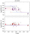 |
Fig. 1. 12+log(O/H) and 12+log(N/H) vs. surface gravity in the field and cluster stars. The circles represent single measurements, while the squares represent the results binned in log g bins of 0.5. The curves indicate the model of Lagarde et al. (2012) for 1 M ⊙ (red dashed indicates ST, red continuous indicates TCR), 2 M⊙ (black dashed indicates ST, black continuous indicates TCR) and 3 M⊙ (blue continuous indicates TCR). |
In the bottom panel of Fig. 1, we show oxygen abundances versus surface gravity. In this case, the effect of mixing is negligible both from models and observations. Thus the measured oxygen abundance can be considered representative of the initial composition of the stars. We note, however, a relevant spread in the O abundances possibly related to two different points: firstly, the presence of both thin and thick disc stars, of which the latter is more enhanced in O/Fe with respect to the thin disc stars; and secondly, the missing correction of telluric absorption, which is not included in the Gaia-ESO standard reduction.
We also investigated the effect of metallicity in the enhancement of nitrogen (and of oxygen) during stellar evolution to see if we are allowed to apply, in first approximation, an average correction to our stars, which span a metallicity range of about ~1 dex. In Fig. 2, we show the variation of surface abundances of nitrogen and oxygen at different metallicities for three representative stellar masses (1, 1.25 and 2 M⊙) using the ST models of Lagarde et al. (2012). In our metallicity range (0.005 ≤ Z ≤ 0.015) there are no strong variations of ΔN/H = N/Hfinal–N/Hinitial and an average value of 0.25 dex is a good approximation for low mass stars, i.e. mostly representative of the field thin and thick disc populations.
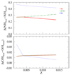 |
Fig. 2. Δ N/H = N/H final–N/H initial and Δ O/H = O/H final–O/H initial vs. Z metallicity in the ST models of Lagarde et al. (2012) for stars of 1, 1.25, and 2 M ⊙. |
On the other hand, for the open clusters, the average correction valid for field stars is, in general, an under-estimation since they are younger and thus their evolved stars are more massive. Using the mass at turn-off of clusters uniformly derived Parsec isochrones (Bressan et al. 2012) with the ages and metallicities of Table 2, we estimate the variation of nitrogen surface abundance during stellar evolution using the models of Lagarde et al. (2012) for more massive stars. In Fig. 3 we plot ΔN/H = N/Hfinal−N/Hinitial as a function of stellar mass for solar metallicity. The variation ΔN/H is larger for more massive stars and it can be approximated with a polynomial fit. A fit to the data of Fig. 3 gives us the possibility to correct the N/H abundances for giant stars in clusters for which we know the turn-off mass. The fit is given in the following equation, where m is the turn-off mass:
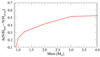 |
Fig. 3. Δ N/H = N/H final–N/H initial vs. mass in the ST models of Lagarde et al. (2012) at solar metallicity. |
 (1)
(1)
In the following plots and discussions, we applied a correction to 12+log(N/H) abundances and to N/O abundance ratios, both in clusters and field stars. For the field population, we considered a constant correction of −0.25 dex, while for the cluster stars we used the fit in Eq. (1) using the turn-off masses of Table 1. The errors due to this correction are difficult to estimate and they are not propagated in the final abundances. In the following analysis, for both populations we only considered stars with log g ≤ 3.5 dex, which have a more reliable determination of O and N abundances.
5. Abundance results
In Fig. 4 we compare our results, after correcting nitrogen abundances for the effects of stellar evolution, with those collected by Israelian et al. (2004) for both metal-poor and metal-rich dwarf stars. On the one hand, in the metallicity interval -0.5 < [Fe/H] < 0.5 spanned by our new data, there is a very good agreement between the GES and the literature results. On the other hand, the sample of Israelian et al. (2004) reaches very low metallicities that are not available in our sample dominated by the disc populations.
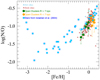 |
Fig. 4. log(N/O) vs. [Fe/H] in our samples compared with the literature data of Israelian et al. (2004). Open clusters are shown with large filled circle (in green clusters with RGC > 7 kpc and in orange clusters with RGC ≤ 7 kpc), thin and thick disc stars are represented with smaller light blue and pink triangles, respectively. The literature sample of Israelian et al. (2004) is represented with cyan squares. |
In Fig. 5, we show [N/Fe] and [O/Fe] as function of [Fe/H] in the thin and thick disc populations and in open clusters. We performed the two-dimensional Kolmogorov-Smirnov (KS) test (Fasano & Franceschini 1987) to quantify the probability that the abundance ratios in the three populations derive from similar distributions.
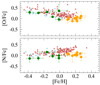 |
Fig. 5. [N/Fe] and [O/Fe] as function of [Fe/H] in the thin and thick disc populations and in open clusters. Symbols and colour codes as in Fig. 4. |
The bi-dimensional KS statistical test is the generalisation of the classical one-dimensional KS test and it is used to analyse two-or three-dimensional samples. Based on the two-dimensional KS test, the significance of the equivalence between the distributions of [O/Fe] and of [N/Fe] in thin disc stars with thick disc stars is less than 1% in the overlapping metallicity region. On the other hand, the abundance ratios [N/Fe] and [O/Fe] in open clusters are much similar to those in thin disc stars with probabilities ranging from ~20% to ~50%, respectively.
6. Chemical evolution models
We compare our observed data sample with the predictions of classical one-zone chemical evolution models, taking a very similar approach as in Vincenzo et al. (2016) with standard assumptions that are used to reproduce the main characteristics of our Galaxy. The parameters of our reference model are in agreement with many previous studies (e.g. Minchev et al. 2013; Spitoni et al. 2015, 2018).
In summary, the SFR is assumed to follow a linear Schmidt-Kennicutt law, namely SFR(t) = SFE × M
gas(t), where SFE represents the star formation efficiency, a free parameter of our models, and Mgas(t) is the total amount of gas in the galaxy at the time t. We assume the Galactic disc to assemble by accreting primordial gas with a rate exponentially decaying as a function of time, namely I(t) ∝ exp(−t/τ), normalised such that  , where τ represents the so-called infall timescale, a free parameter of our models, and Minf the integrated amount of gas accreted into the Galactic potential well during the Galaxy lifetime (tG = 14 Gyr); in this work, we assume log(Minf) = 11.5 dex.
In this work, the effect of galactic winds is included, by assuming that the outflow rate is directly proportional to the SFR, namely O(t) = w × SFR(t), where w represents the so-called mass loading factor, another free parameter of our models. The wind is differential and it is assumed to carry only the main nucleosynthetic products of SNe, hence α- and iron-peak elements. To compute the time of onset of the galactic wind, we follow the same formalism as in Bradamante et al. (1998). Finally, we assume the initial mass function (IMF) of Salpeter (1955).
For LIMS, we assume the same stellar yields as in Vincenzo et al. (2016), while for massive stars the stellar yields of Kobayashi et al. (2011). In order to reproduce the low-metallicity N/O plateau, we assume that massive stars only produce primary N with an empirical stellar yield that is computed as in Vincenzo et al. (2016). For Type Ia SNe, we assume the following delay time distribution function (DTD): DTDIa(t) ∝ 1/t (Totani et al. 2008), which gives very similar results as the DTD of Schönrich & Binney (2009), and nucleosynthetic yields from Iwamoto et al. (1999). The assumed DTD is normalised to have a total number of SNe in the range ~1−2 SNe per 103 M⊙ of stellar mass formed for all our models (Bell et al. 2003; Maoz et al. 2014). Finally, we assume the metallicity-dependent stellar lifetimes of Kobayashi (2004).
We made several numerical experiments, by assuming different prescriptions for Type Ia SNe, IMF, and stellar yields, and we came to the conclusion that the aforementioned assumptions provide the best match to the observed data sample for [O/Fe] versus [Fe/H] and log(N/O) versus [Fe/H].
We construct a grid of chemical evolution models by continuously varying the free parameters in the following ranges: 0.2 ≤ SFE ≤ 4 Gyr−1, 1 ≤ τ ≤ 12 Gyr and 0.4 ≤ w ≤ 1.0. In the next section, when we refer to our reference grid of models, we mean the aforementioned variation of the free parameters. Our reference chemical evolution model assumes SFE = 1 Gyr−1, τ = 7 Gyr and w = 0.8, which can reproduce the observed average [O/Fe]–[Fe/H] and N/O–[Fe/H] abundance patterns.
The main differences between the chemical evolution models of Vincenzo et al. (2016) and those of this work can be summarised as follows. Firstly, we assume the IMF of Salpeter (1955), containing a lower number of LIMS than the Kroupa et al. (1993) IMF assumed in Vincenzo et al. (2016). Secondly, we assume the double degenerate scenario for Type Ia SNe, while Vincenzo et al. (2016) assume the single-degenerate scenario of Matteucci & Recchi (2001).
The main limitation of our approach is that we adopt a one-zone model to characterise the whole disc of our Galaxy, varying the main free parameters to reproduce the observed chemical abundance patterns. There are chemical abundance gradients in our Galaxy (see e.g. Esteban & García-Rojas 2018), which can also be seen in our dataset and can be better understood – from a physical point of view – only by making use of chemodynamical simulations embedded in a cosmological framework (e.g. Kobayashi & Nakasato 2011; Vincenzo & Kobayashi 2018). Finally, we assume in our model a single onset for the galactic wind, which is maintained continuously afterwards; this may not be entirely appropriate for actively star-forming galaxies that may experience large variations in their SFRs.
7. Results
In Fig. 6, we compare log(N/O) versus [Fe/H] of field stars (divided in thin and thick disc) and the open clusters with the set of chemical evolution models from our grid. In all panels we also report the reference model. First we note the clusters and stars of the Milky Way are located in the top right portion of the plot, where the secondary production of N dominates. Conversely to studies of unresolved galaxies, the stellar population of the Milky Way allows us to appreciate the spanned ranges of metallicities and of log(N/O) belonging to the same galaxy. Thanks to the precise measurements of distances of open clusters, we can also relate the variation of N/O to various sections of the Galaxy.
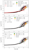 |
Fig. 6. log(N/O) versus [Fe/H] with open clusters shown as large filled circle (in green clusters with RGC > 7 kpc and in orange clusters with RGC ≤ 7 kpc), individual measurements of thin and thick disc stars are represented with cyan and pink triangles, respectively. In the top panel, we present the grid of models in which we vary the SFE; in the central panel, the infall timescale is changed, while in the bottom panel, the outflow loading factor is varied. In each panel, the reference model is identified with a solid line. |
In the top panel, we vary the SFE, from 0.2 Gyr−1 to 4 Gyr−1. As discussed in Vincenzo et al. (2016), the effect of varying SFE is to increase the metal content and thus to move the point where the secondary component of N starts to contribute. As aforementioned, since we assume an IMF that is not bottom heavy (Salpeter 1955), the N production from LIMS is less prominent than in Vincenzo et al. (2016). The onset of the galactic wind in the models is crucially determined by the interplay between the injection rate of thermal energy by SN events and stellar winds and the assembly of the Galaxy potential well as a function of time (mostly regulated by the assumed infall mass and infall timescale). By lowering the SFE in the model (keeping the other parameters fixed), there is less thermal energetic feedback from SNe and stellar winds at any time of the galaxy evolution, delaying the onset of the galactic wind towards higher [Fe/H] abundances. We remark the fact that the galactic wind onset in Fig. 6 appears as a sudden increase in log(N/O), from a given [Fe/H] on. To reproduce the range of log(N/O) spanned by the observations, a variety of SFE is necessary. In particular, to reproduce the observed abundances in the thin disc stars, we need higher average SFEs than for thick disc stars. Here and in the following discussion we consider that young and intermediate-age open clusters are not affected by strong radial migration and thus they are representative of the abundances of the places where they are observed (cf. e.g. Quillen et al. 2018).
In the central panel, we vary the infall timescale from 1 Gyr to 10 Gyr, keeping the SFE fixed at its reference values. The main effect of the infall timescale is that models with longer infall timescales have a galactic wind that develops at earlier times, and thus the location of the break point due to the onset of the wind (see Fig. 3 of V16) is moved and the slopes of the models after the break point are changed. The Milky Way resolved data are better reproduced by models with longer infall timescales in agreement with other evidence of timescales of the order of ~8 Gyr of the Galactic thin disc at solar Galactocentric distance. The inner disc open clusters can be better reproduced with models with shorter infall timescales, while the outer disc open clusters need a longer infall timescale in agreement with the insideout scenario. The assumption of infall timescales τinf > 7 Gyr has little effect on the chemical evolution tracks in Fig. 6, for a fixed SFE, confirming that the main parameter in our model to discriminate between thin and thick disc stars is given by the SFE.
In the bottom panel, we vary the effects of differential outflow, the so-called outflow loading factor. In our models, we assume a differential outflow, which carries out only the main nucleosynthetic products of SNe, thus affecting oxygen, but not nitrogen. In the plot, we vary it from ω = 0.4 to ω = 1.0, while the reference model has ω = 0.8. In the case of the Milky Way, a ω = 1.0 is better suited to reproduce the high metallicity data of field stars, while for the inner disc clusters a lower loading factor is needed (see Fig. 6, bottom panel). This may be justified by the fact that the ISM in innermost regions of our Galaxy is more tightly bound than in the outermost regions and is eventually ejected with higher average efficiencies.
Although our model might be simplistic, it can capture some of the main features of the observed chemical abundance data. We remark that by moving along each chemical evolution track in Fig. 6, the SFR and hence the predicted number of stars with a given log(N/O) and [Fe/H] can vary; hence there is a third hidden dimension in the tracks of Fig. 6. For example, the model with the lowest SFE in the top panel contains very few stars after the onset of the galactic wind; conversely, the model with the shortest infall timescale in the middle panel contains a large number of stars also after the development of the galactic wind. Therefore, even though SFE and infall timescale seem to suffer from some degeneracies in the chemical evolution tracks of Fig. 6, their relative contributions might be better discriminated by looking at the number of stars with a given log(N/O) and [Fe/H] in the model and data as well. Nevertheless, to do this kind of study, we need a much larger and more complete statistical dataset of chemical abundances in our Galaxy than that presented by this work. Large datasets are currently available, for example from APOGEE, GALAH, and LAMOST (Majewski et al. 2017; De Silva et al. 2015; Luo et al. 2015), however, they suffer from lower resolution than in this work.
Putting together all these considerations, we can conclude that the reference model alone is not able to reproduce the whole abundance ratios along the radial range of the disc. Because of radial variations of the Galactic properties and to the inside-out formation of the disc, this is indeed expected. The more efficient way to reproduce the abundance ratios in the outermost clusters is by assuming relatively long infall timescales (τ inf ~ 7−8 Gyr) and SFEs of the order of unity per Gyr, which is perfectly in line with the inside-out scenario for the formation of the Milky Way disc. We find that thin disc stars tend to have higher log(N/O) at fixed log(O/H)+12 than thick disc stars; this can be reproduced only by assuming for thin disc stars higher average SFEs and longer infall timescales, which has the effect that the SFE is more important than the effect of the infall timescale. Finally, lower outflow loading factors also seem to reproduce better the abundance patterns in the inner open clusters.
8. Milky Way in the extragalactic framework
In Fig. 7, we compare our results (right panel) with the MaNGA sample (Belfiore et al. 2017), which includes 550 resolved galaxies with stellar masses between 109 and 1011M⊙ (left panel). The Milky Way stellar data span an interval in log(N/O) as large as the whole range spanned by external galaxies belonging to various bins of stellar masses. The stellar mass of our Galaxy is estimated to be 6.1 ± 1.1 × 10¹⁰M⊙ (Licquia & Newman 2015). The bulk of the thick disc stars and the innermost clusters are indeed in agreement with log(N/O) of external galaxies in the stellar mass bin 10.50–10.75. On the other hand, the outer regions of the Milky Way show log(N/O) values consistent with those of low stellar mass galaxies, in which the SFE is typically lower. In addition, in the very inner clusters and in high metallicity thick disc stars, we observe the highest values of log(N/O), reached in inner parts of the more massive star-forming galaxies. Such high values are also reached in resolved H II regions of nearby galaxies (see e.g. Fig. 6 of Bresolin et al. (2004) where measurements in M 51, M 101 and NGC 2403 are shown). The radial variation of log(N/O) in the Galaxy can be interpreted as a consequence of the different SFE, infall timescales, and galactic wind between the central and outer regions of discs. This is not limited to the H II regions but also Galactic stellar populations keep traces of the different mechanisms of formation of various regions of the Milky Way.
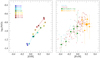 |
Fig. 7. Left panel: log(N/O) vs. [O/H] as a function of both stellar mass and radius in the sample of resolved galaxies of Belfiore et al. (2017; extracted from their Fig. 8). For each mass bin (see the legend for the range in logarithm of the stellar mass of each bin) the uppermost star represents the innermost radial bin (0.0–0.25 Re while the lower star represents the outermost radial bin (1.75–2.0 Re). Right panel: log(N/O) vs. [Fe/H] in our Milky Way samples of field stars (blue and pink triangles, thin and thick discs, respectively) and of open clusters (in green clusters with R GC > 7 kpc and in orange clusters with RGC ≤ 7 kpc). |
9. Summary and conclusions
We present the Gaia-ESO IDR2-3, IDR4, IDR5 abundances of N and O in open clusters and in field stars belonging to thin and thick discs. We estimate the effect of stellar evolution on N abundance, and we correct the abundance of giant stars making use of the stellar evolution models of Lagarde et al. (2012). The study of individual stars and clusters has shown that the stellar populations of the Milky Way present a wide range of log(N/O), mainly located in the region dominated by the secondary production of N. This distribution is comparable to their range observed in individual HII regions in external massive galaxies, or even larger (e.g. Bresolin et al. 2004). We compare log(N/O) versus [Fe/H] in our samples with a grid of chemical evolution models, based on the models of Vincenzo et al. (2016). The Galactic reference model alone is not able to reproduce all the resolved Galactic trends. We need a higher SFE and/or a longer infall timescale in the outskirts to reproduce the abundance ratios in the outer regions, coupled with a shorter infall timescale in the inner regions together with a lower outflow loading factor to explain the abundance ratios in the inner disc. This is in line with the request of an inside-out formation in the Milky Way disc. Interestingly, thin disc stars have higher average log(N/O) ratios at fixed log(O/H)+12 than thick disc stars; this feature can be better reproduced by models assuming higher average SFEs for thin disc stars. We also compared our resolved Milky Way results with the local Universe sample of MaNGA, finding a remarkably good agreement, but with the Milky Way data spanning a larger range of log(N/O) than integrated observations of galaxies of similar stellar mass.
Acknowledgments
We thank the referee for her/his constructive report that improved the quality and presentation of the paper. We thank Viviana Casasola for her help the KS bi-dimensional test. This work is based on data products from observations made with ESO Telescopes at the La Silla Paranal Observatory under programme ID 188.B-3002. These data products have been processed by the Cambridge Astronomy Survey Unit (CASU) at the Institute of Astronomy, University of Cambridge, and by the FLAMES/UVES reduction team at INAF/Osservatorio Astrofisico di Arcetri. These data have been obtained from the Gaia-ESO Survey Data Archive, prepared and hosted by the Wide Field Astronomy Unit, Institute for Astronomy, University of Edinburgh, which is funded by the UK Science and Technology Facilities Council (STFC). This work was partly supported by the European Union FP7 programme through ERC grant number 320360 and by the Leverhulme Trust through grant RPG-2012-541. We acknowledge the support from INAF and Ministero dell’ Istruzione, dell’ Università’ e della Ricerca (MIUR) in the form of the grant “Premiale VLT 2012”. The results presented here benefit from discussions held during the Gaia-ESO workshops and conferences supported by the ESF (European Science Foundation) through the GREAT Research Network Programme. FV acknowledges funding from the UK STFC through grant ST/M000958/1. T.B. was supported by the project grant “The New Milky Way” from the Knut and Alice Wallenberg Foundation. A.B. acknowledges support from the Millennium Science Initiative (Chilean Ministry of Economy). GT, AD, ŠM, RM, ES, and VB acknowledge support from the European Social Fund via the Lithuanian Science Council grant No.09.3.3-LMT-K-712-01-0103.
References
- Abazajian, K. N. Adelman-McCarthy, J. K., Agüeros, M. A., et al. 2009, ApJ, 182, 543 [Google Scholar]
- Adibekyan, V. Z., Santos, N. C., Sousa, S. G., & Israelian, G. 2011, A&A, 535, L11 [NASA ADS] [CrossRef] [EDP Sciences] [Google Scholar]
- Alvarez, R., & Plez, B. 1998, A&A, 330, 1109 [NASA ADS] [Google Scholar]
- Asplund, M., Grevesse, N., Sauval, A. J., & Scott, P. 2009, ARA&A, 47, 481 [NASA ADS] [CrossRef] [Google Scholar]
- Belfiore, F., Maiolino, R., Tremonti, C., et al. 2017, MNRAS, 469, 151 [NASA ADS] [CrossRef] [Google Scholar]
- Bell, E. F., McIntosh, D. H., Katz, N., & Weinberg, M. D. 2003, ApJS, 149, 289 [NASA ADS] [CrossRef] [Google Scholar]
- Berg, D. A., Skillman, E. D., Marble, A. R., et al. 2012, ApJ, 754, 98 [NASA ADS] [CrossRef] [Google Scholar]
- Bradamante, F., Matteucci, F., & D’Ercole, A. 1998, A&A, 337, 338 [NASA ADS] [Google Scholar]
- Bresolin, F., Garnett, D. R., & Kennicutt, R. C., Jr. 2004, ApJ, 615, 228 [NASA ADS] [CrossRef] [Google Scholar]
- Bressan, A., Marigo, P., Girardi, L., et al. 2012, MNRAS, 427, 127 [NASA ADS] [CrossRef] [Google Scholar]
- Bundy, K., Bershady, M. A., Law, D. R., et al. 2015, ApJ, 798, 7 [NASA ADS] [CrossRef] [Google Scholar]
- Carigi, L., Peimbert, M., Esteban, C., & García-Rojas, J. 2005, ApJ, 623, 213 [NASA ADS] [CrossRef] [Google Scholar]
- Casagrande, L., Silva Aguirre, V., Stello, D., et al. 2014, ApJ, 787, 110 [NASA ADS] [CrossRef] [Google Scholar]
- Casagrande, L., Silva Aguirre, V., Schlesinger, K. J., et al. 2016, MNRAS, 455, 987 [NASA ADS] [CrossRef] [Google Scholar]
- Chiappini, C., Matteucci, F., & Gratton, R. 1997, ApJ, 477, 765 [NASA ADS] [CrossRef] [Google Scholar]
- Chiappini, C., Matteucci, F., & Romano, D. 2001, ApJ, 554, 1044 [NASA ADS] [CrossRef] [Google Scholar]
- Chiappini, C., Matteucci, F., & Ballero, S. K. 2005, A&A, 437, 429 [NASA ADS] [CrossRef] [EDP Sciences] [Google Scholar]
- Chieffi, A., & Limongi, M. 2004, ApJ, 608, 405 [NASA ADS] [CrossRef] [Google Scholar]
- Chieffi, A., & Limongi, M. 2013, ApJ, 764, 21 [NASA ADS] [CrossRef] [Google Scholar]
- Christlieb, N., Beers, T. C., Barklem, P. S., et al. 2004, A&A, 428, 1027 [NASA ADS] [CrossRef] [EDP Sciences] [Google Scholar]
- Contini, M. 2015, MNRAS, 452, 3795 [NASA ADS] [CrossRef] [Google Scholar]
- Contini, M. 2016, MNRAS, 460, 3232 [NASA ADS] [CrossRef] [Google Scholar]
- Contini, M. 2017a, MNRAS, 466, 2787 [NASA ADS] [CrossRef] [Google Scholar]
- Contini, M. 2017b, MNRAS, 469, 3125 [NASA ADS] [CrossRef] [Google Scholar]
- Contini, M. 2018, ArXiv e-prints [arXiv:1801.03312] [Google Scholar]
- Contini, T., Treyer, M. A., Sullivan, M., & Ellis, R. S. 2002, MNRAS, 330, 75 [NASA ADS] [CrossRef] [Google Scholar]
- De Silva, G. M., Freeman, K. C., Bland-Hawthorn, J., et al. 2015, MNRAS, 449, 2604 [NASA ADS] [CrossRef] [MathSciNet] [Google Scholar]
- Ecuvillon, A., Israelian, G., Santos, N. C., et al. 2004, A&A, 418, 703 [NASA ADS] [CrossRef] [EDP Sciences] [Google Scholar]
- Esteban, C., & García-Rojas, J. 2018, MNRAS, 478, 2315 [NASA ADS] [CrossRef] [Google Scholar]
- Esteban, C., García-Rojas, J., Peimbert, M., et al. 2005, ApJ, 618, L95 [NASA ADS] [CrossRef] [Google Scholar]
- Fasano, G., & Franceschini, A. 1987, MNRAS, 225, 155 [NASA ADS] [CrossRef] [Google Scholar]
- Feuillet, D. K., Bovy, J., Holtzman, J., et al. 2018, MNRAS, 477, 2326 [NASA ADS] [CrossRef] [Google Scholar]
- Gaia Collaboration (Prusti, T., et al.) 2016, A&A, 595, A1 [NASA ADS] [CrossRef] [EDP Sciences] [Google Scholar]
- Gaia Collaboration (Brown, A. G. A., et al.) 2018, A&A, 616, A1 [NASA ADS] [CrossRef] [EDP Sciences] [Google Scholar]
- Gavilán, M., Mollá, M., & Buell, J. F. 2006, A&A, 450, 509 [NASA ADS] [CrossRef] [EDP Sciences] [Google Scholar]
- Gilmore, G., Randich, S., Asplund, M., et al. 2012, The Messenger, 147, 25 [NASA ADS] [Google Scholar]
- Gil-Pons, P., Doherty, C. L., Lau, H., et al. 2013, A&A, 557, A106 [NASA ADS] [CrossRef] [EDP Sciences] [Google Scholar]
- Gonzalez, G., Laws, C., Tyagi, S., & Reddy, B. E. 2001, AJ, 121, 432 [NASA ADS] [CrossRef] [Google Scholar]
- Grevesse, N., Asplund, M., & Sauval, A. J. 2007, Space Sci. Rev., 130, 105 [Google Scholar]
- Gustafsson, B., Edvardsson, B., Eriksson, K., et al. 2008, A&A, 486, 951 [NASA ADS] [CrossRef] [EDP Sciences] [Google Scholar]
- Henry, R. B. C., Edmunds, M. G., & Köppen, J. 2000, ApJ, 541, 660 [NASA ADS] [CrossRef] [Google Scholar]
- Israelian, G., Ecuvillon, A., Rebolo, R., et al. 2004, A&A, 421, 649 [NASA ADS] [CrossRef] [EDP Sciences] [Google Scholar]
- Iwamoto, K., Brachwitz, F., Nomoto, K., et al. 1999, ApJS, 125, 439 [NASA ADS] [CrossRef] [MathSciNet] [Google Scholar]
- Izotov, Y. I., Thuan, T. X., & Guseva, N. G. 2012, A&A, 546, A122 [NASA ADS] [CrossRef] [EDP Sciences] [Google Scholar]
- James, B. L., Koposov, S., Stark, D. P., et al. 2015, MNRAS, 448, 2687 [NASA ADS] [CrossRef] [Google Scholar]
- Johansson, S., Litzen, U., Lundberg, H., & Zhang, Z. 2003, ApJ, 584, L107 [NASA ADS] [CrossRef] [Google Scholar]
- Kewley, L. J., & Ellison, S. L. 2008, ApJ, 681, 1204 [Google Scholar]
- Kobayashi, C. 2004, MNRAS, 347, 740 [NASA ADS] [CrossRef] [Google Scholar]
- Kobayashi, C., & Nakasato N. 2011, ApJ, 729, 16 [NASA ADS] [CrossRef] [Google Scholar]
- Kobayashi, C., Karakas A. I., & Umeda H. 2011, MNRAS, 414, 3231 [NASA ADS] [CrossRef] [Google Scholar]
- Kordopatis, G., Recio-Blanco, A., de Laverny, P., et al. 2011, A&A, 535, A107 [NASA ADS] [CrossRef] [EDP Sciences] [Google Scholar]
- Kordopatis, G., Wyse, R. F. G., Gilmore, G., et al. 2015, A&A, 582, A122 [NASA ADS] [CrossRef] [EDP Sciences] [Google Scholar]
- Kroupa, P., Tout C. A., & Gilmore G. 1993, MNRAS, 262, 545 [NASA ADS] [CrossRef] [Google Scholar]
- Kumari, N., James, B. L., Irwin, M. J., Amorín, R., & Pérez-Montero, E. 2018, MNRAS, 476, 3793 [NASA ADS] [CrossRef] [Google Scholar]
- Kurucz, R. L. 2005, Mem. Soc. Astron. It. Suppl., 8, 189 [Google Scholar]
- Lagarde, N., Decressin, T., Charbonnel, C., et al. 2012, A&A, 543, A108 [NASA ADS] [CrossRef] [EDP Sciences] [Google Scholar]
- Lagarde, N., Reylé, C., Robin, A. C., et al. 2018, A&A, in press, DOI: 10.1051/0004-6361/201732433 [Google Scholar]
- Liang, Y. C., Zhao, G., & Shi, J. R. 2001, A&A, 374, 936 [NASA ADS] [CrossRef] [EDP Sciences] [Google Scholar]
- Liang, Y. C., Yin, S. Y., Hammer, F., et al. 2006, ApJ, 652, 257 [NASA ADS] [CrossRef] [Google Scholar]
- Licquia, T. C., & Newman, J. A. 2015, ApJ, 806, 96 [NASA ADS] [CrossRef] [Google Scholar]
- Lindegren, L., Lammers, U., Bastian, U., et al. 2016, A&A, 595, A4 [NASA ADS] [CrossRef] [EDP Sciences] [Google Scholar]
- López-Sánchez, Á. R., Dopita, M. A., Kewley, L. J., et al. 2012, MNRAS, 426, 2630 [NASA ADS] [CrossRef] [Google Scholar]
- Luo, A.-L., Zhao, Y.-H., Zhao, G., et al. 2015, Res. Astron. Astrophy., 15, 1095 [CrossRef] [Google Scholar]
- Majewski, S. R., Schiavon, R. P., Frinchaboy, P. M., et al. 2017, AJ, 154, 94 [NASA ADS] [CrossRef] [Google Scholar]
- Magrini, L., Randich, S., Kordopatis, G., et al. 2017, A&A, 603, A2 [NASA ADS] [CrossRef] [EDP Sciences] [Google Scholar]
- Magrini, L., Spina, L., Randich, S., et al. 2018, A&A, 617, A106 [NASA ADS] [CrossRef] [EDP Sciences] [Google Scholar]
- Maiolino, R., Nagao, T., Grazian, A., et al. 2008, A&A, 488, 463 [NASA ADS] [CrossRef] [EDP Sciences] [Google Scholar]
- Maoz, D., Mannucci, F., & Nelemans, G. 2014, ARA&A, 52, 107 [NASA ADS] [CrossRef] [Google Scholar]
- Martig, M., Fouesneau, M., Rix, H.-W., et al. 2016, MNRAS, 456, 3655 [NASA ADS] [CrossRef] [Google Scholar]
- Masseron, T., & Gilmore, G. 2015, MNRAS, 453, 1855 [NASA ADS] [CrossRef] [Google Scholar]
- Matteucci, F., & Recchi, S. 2001, ApJ, 558, 351 [NASA ADS] [CrossRef] [Google Scholar]
- Meynet, G., & Maeder, A. 2000, A&A, 361, 101 [NASA ADS] [Google Scholar]
- Meynet, G., & Maeder, A. 2002a, A&A, 381, L25 [NASA ADS] [CrossRef] [EDP Sciences] [Google Scholar]
- Meynet, G., & Maeder, A. 2002b, A&A, 390, 561 [NASA ADS] [CrossRef] [EDP Sciences] [Google Scholar]
- Minchev, I., Chiappini, C., & Martig, M. 2013, A&A, 558, A9 [NASA ADS] [CrossRef] [EDP Sciences] [Google Scholar]
- Mollá, M., Vílchez, J. M., Gavilán, M., & Díaz, A. I. 2006, MNRAS, 372, 1069 [NASA ADS] [CrossRef] [Google Scholar]
- Pagel, B. E. J., Simonson, E. A., Terlevich, R. J., & Edmunds, M. G. 1992, MNRAS, 255, 325 [NASA ADS] [CrossRef] [Google Scholar]
- Pasquini, L., Avila, G., Blecha, A., et al. 2002, The Messenger, 110, 1 [NASA ADS] [Google Scholar]
- Peña-Guerrero, M. A., Peimbert, A., & Peimbert, M. 2012, ApJ, 756, L14 [NASA ADS] [CrossRef] [Google Scholar]
- Perez-Montero, E., & Contini, T. 2009, MNRAS, 398, 949 [NASA ADS] [CrossRef] [Google Scholar]
- Pettini, M., Ellison, S. L., Bergeron, J., & Petitjean, P. 2002, A&A, 391, 21 [NASA ADS] [CrossRef] [EDP Sciences] [MathSciNet] [Google Scholar]
- Pettini, M., Zych, B. J., Steidel, C. C., & Chaffee, F. H. 2008, MNRAS, 385, 2011 [NASA ADS] [CrossRef] [Google Scholar]
- Pilyugin, L. S., Vílchez, J. M., & Thuan, T. X. 2010, ApJ, 720, 1738 [NASA ADS] [CrossRef] [Google Scholar]
- Quillen, A. C., Nolting, E., Minchev, I., De Silva, G., & Chiappini, C. 2018, MNRAS, 475, 4450 [NASA ADS] [CrossRef] [Google Scholar]
- Randich, S., Gilmore, G., & Gaia-ESO Consortium 2013, The Messenger, 154, 47 [NASA ADS] [Google Scholar]
- Renzini, A., & Voli, M. 1981, A&A, 94, 175 [NASA ADS] [Google Scholar]
- Rudolph, A. L., Fich, M., Bell, G. R., et al. 2006, ApJS, 162, 346 [NASA ADS] [CrossRef] [Google Scholar]
- Sacco, G. G., Morbidelli, L., Franciosini, E., et al. 2014, A&A, 565, A113 [NASA ADS] [CrossRef] [EDP Sciences] [Google Scholar]
- Sadakane, K., Ohkubo, M., Takeda, Y., et al. 2002, PASJ, 54, 911 [NASA ADS] [CrossRef] [Google Scholar]
- Salaris, M., Pietrinferni, A., Piersimoni, A. M., & Cassisi, S. 2015, A&A, 583, A87 [NASA ADS] [CrossRef] [EDP Sciences] [Google Scholar]
- Salpeter, E. E. 1955, ApJ, 121, 161 [Google Scholar]
- Santos, N. C., Israelian, G., & Mayor, M. 2000, A&A, 363, 228 [NASA ADS] [Google Scholar]
- Schönrich, R., & Binney, J. 2009, MNRAS, 396, 203 [NASA ADS] [CrossRef] [Google Scholar]
- Smiljanic, R., Korn, A. J., Bergemann, M., et al. 2014, A&A, 570, A122 [NASA ADS] [CrossRef] [EDP Sciences] [Google Scholar]
- Spite, M., Cayrel, R., Plez, B., et al. 2005, A&A, 430, 655 [NASA ADS] [CrossRef] [EDP Sciences] [Google Scholar]
- Spitoni, E., Romano, D., Matteucci, F., & Ciotti, L. 2015, ApJ, 802, 129 [NASA ADS] [CrossRef] [Google Scholar]
- Spitoni, E., Matteucci, F., Jönsson, H., Ryde, N., & Romano, D. 2018, A&A, 612, A16 [NASA ADS] [CrossRef] [EDP Sciences] [Google Scholar]
- Stonkutė, E., Koposov, S. E., Howes, L. M., et al. 2016, MNRAS, 460, 1131 [NASA ADS] [CrossRef] [Google Scholar]
- Suárez-Andrés, L., Israelian, G., González Hernández, J. I., et al. 2016, A&A, 591, A69 [NASA ADS] [CrossRef] [EDP Sciences] [Google Scholar]
- Takahashi, K., Umeda, H., & Yoshida, T. 2014, ApJ, 794, 40 [NASA ADS] [CrossRef] [Google Scholar]
- Takeda, Y., Sato, B., Kambe, E., et al. 2001, PASJ, 53, 1211 [NASA ADS] [CrossRef] [Google Scholar]
- Tautvaišienė, G., Drazdauskas, A., Mikolaitis, Š., et al. 2015, A&A, 573, A55 [NASA ADS] [CrossRef] [EDP Sciences] [Google Scholar]
- Totani, T., Morokuma, T., Oda, T., Doi, M., & Yasuda, N. 2008, PASJ, 60, 1327 [NASA ADS] [CrossRef] [Google Scholar]
- van den Hoek, L. B., & Groenewegen, M. A. T. 1997, A&AS, 123, 305 [NASA ADS] [CrossRef] [EDP Sciences] [Google Scholar]
- Vangioni, E., Dvorkin, I., Olive, K. A., et al. 2018, MNRAS, 477, 56 [NASA ADS] [CrossRef] [Google Scholar]
- van Zee, L., & Haynes, M. P. 2006, ApJ, 636, 214 [NASA ADS] [CrossRef] [Google Scholar]
- van Zee, L., Salzer, J. J., & Haynes, M. P. 1998, ApJ, 497, L1 [NASA ADS] [CrossRef] [Google Scholar]
- Vila-Costas, M. B., & Edmunds, M. G. 1992, MNRAS, 259, 121 [NASA ADS] [CrossRef] [Google Scholar]
- Vincenzo, F., & Kobayashi, C. 2018, MNRAS, 478, 155 [NASA ADS] [CrossRef] [Google Scholar]
- Vincenzo, F., Belfiore, F., Maiolino, R., Matteucci, F., & Ventura, P. 2016, MNRAS, 458, 3466 [NASA ADS] [CrossRef] [Google Scholar]
- Weinberg, D. H., Andrews, B. H., & Freudenburg, J. 2017, ApJ, 837, 183 [NASA ADS] [CrossRef] [Google Scholar]
- Zafar, T., Centurión, M., Péroux, C., et al. 2014, MNRAS, 444, 744 [NASA ADS] [CrossRef] [Google Scholar]
Appendix A: Stellar parameters and abundances of individual stars
In this appendix, we present the stellar parameters and abundances used in the present work. The complete database for DR5 is available on-line in the ESO portal.
Thin and thick disc star parameters and abundances.
All Tables
All Figures
|
Fig. 1. 12+log(O/H) and 12+log(N/H) vs. surface gravity in the field and cluster stars. The circles represent single measurements, while the squares represent the results binned in log g bins of 0.5. The curves indicate the model of Lagarde et al. (2012) for 1 M ⊙ (red dashed indicates ST, red continuous indicates TCR), 2 M⊙ (black dashed indicates ST, black continuous indicates TCR) and 3 M⊙ (blue continuous indicates TCR). |
| In the text | |
|
Fig. 2. Δ N/H = N/H final–N/H initial and Δ O/H = O/H final–O/H initial vs. Z metallicity in the ST models of Lagarde et al. (2012) for stars of 1, 1.25, and 2 M ⊙. |
| In the text | |
|
Fig. 3. Δ N/H = N/H final–N/H initial vs. mass in the ST models of Lagarde et al. (2012) at solar metallicity. |
| In the text | |
|
Fig. 4. log(N/O) vs. [Fe/H] in our samples compared with the literature data of Israelian et al. (2004). Open clusters are shown with large filled circle (in green clusters with RGC > 7 kpc and in orange clusters with RGC ≤ 7 kpc), thin and thick disc stars are represented with smaller light blue and pink triangles, respectively. The literature sample of Israelian et al. (2004) is represented with cyan squares. |
| In the text | |
|
Fig. 5. [N/Fe] and [O/Fe] as function of [Fe/H] in the thin and thick disc populations and in open clusters. Symbols and colour codes as in Fig. 4. |
| In the text | |
|
Fig. 6. log(N/O) versus [Fe/H] with open clusters shown as large filled circle (in green clusters with RGC > 7 kpc and in orange clusters with RGC ≤ 7 kpc), individual measurements of thin and thick disc stars are represented with cyan and pink triangles, respectively. In the top panel, we present the grid of models in which we vary the SFE; in the central panel, the infall timescale is changed, while in the bottom panel, the outflow loading factor is varied. In each panel, the reference model is identified with a solid line. |
| In the text | |
|
Fig. 7. Left panel: log(N/O) vs. [O/H] as a function of both stellar mass and radius in the sample of resolved galaxies of Belfiore et al. (2017; extracted from their Fig. 8). For each mass bin (see the legend for the range in logarithm of the stellar mass of each bin) the uppermost star represents the innermost radial bin (0.0–0.25 Re while the lower star represents the outermost radial bin (1.75–2.0 Re). Right panel: log(N/O) vs. [Fe/H] in our Milky Way samples of field stars (blue and pink triangles, thin and thick discs, respectively) and of open clusters (in green clusters with R GC > 7 kpc and in orange clusters with RGC ≤ 7 kpc). |
| In the text | |
Current usage metrics show cumulative count of Article Views (full-text article views including HTML views, PDF and ePub downloads, according to the available data) and Abstracts Views on Vision4Press platform.
Data correspond to usage on the plateform after 2015. The current usage metrics is available 48-96 hours after online publication and is updated daily on week days.
Initial download of the metrics may take a while.