| Issue |
A&A
Volume 618, October 2018
|
|
|---|---|---|
| Article Number | A176 | |
| Number of page(s) | 9 | |
| Section | The Sun | |
| DOI | https://doi.org/10.1051/0004-6361/201833208 | |
| Published online | 30 October 2018 | |
Effects of electron distribution anisotropy in spectroscopic diagnostics of solar flares
Astronomical Institute of the Czech Academy of Sciences, Fričova 298, 251 65 Ondřejov, Czech Republic
e-mail: This email address is being protected from spambots. You need JavaScript enabled to view it.
Received:
11
April
2018
Accepted:
3
August
2018
Abstract
Aims. We analyzed effects of the bi-Maxwellian electron distribution representing electron temperature anisotropy along and across the magnetic field on the ionization and excitation equilibrium with consequences on the temperature diagnostics of the flare plasma.
Methods. The bi-Maxwellian energy distributions were calculated numerically. Synthetic X-ray line spectra of the bi-Maxwellian distributions were calculated using non-Maxwellian ionization, recombination, excitation and de-excitation rates.
Results. We found that the anisotropic bi-Maxwellian velocity distributions transform to the nonthermal energy distributions with a high-energy tail. Their maximum is shifted to lower energies and contains a higher number of the low-energy particles in comparison with the Maxwellian one. Increasing the deviation of the parameter p = T∥/T⊥ from 1, changes the shape of bi-Maxwellian distributions and ionization equilibrium, and relative line intensities also increase. The effects are more significant for the bi-Maxwellian distribution with T∥ > T⊥. Moreover, considering different acceleration mechanisms and collisional isotropization it is possible that the bi-Maxwellian distributions with high deviations from the Maxwellian distribution are more probable for those with p > 1 than for those with p < 1. Therefore, distributions with p > 1 can be much more easily diagnosed than those with p < 1. Furthermore, we compared the effects of the bi-Maxwellian distributions on the ionization equilibrium and temperature diagnostics with those for the κ-distributions obtained previously. We found that they are similar and at the present state it is difficult to distinguish between the bi-Maxwellian and κ-distributions from the line ratios.
Key words: Sun: flares / Sun: UV radiation / radiation mechanisms: non-thermal
© ESO 2018
1. Introduction
Spectroscopic diagnostics of solar flares revealed that the distributions of electrons in solar flares are non-Maxwellian and exhibit a high-energy tail (e.g., Brown 1971; Krucker et al. 2008; Kašparová & Karlický 2009; Veronig et al. 2010; Zharkova et al. 2011; Kontar et al. 2011; Fletcher et al. 2011; Oka et al. 2013,2015; Simões et al. 2015). To quantify their departure from Maxwellian distribution, a sum of a Maxwellian with a power-law distribution (e.g., Fletcher et al. 2011) or a κ-distribution (e.g., Oka et al. 2013, 2015) are usually used. The expression for the κ-distribution as a function of energy of particles can be found in, for example, Owocki & Scudder (1983), Livadiotis (2015), and Dzifčáková et al. (2015). We note that no anisotropy of the electron distribution in the velocity space is typically assumed.
Bian et al. (2014) have shown that in solar flare conditions the κ-distribution, which is isotropic in velocity space, can be generated. However, in solar flares, especially in the region where the electrons are accelerated, an anisotropy of the electron distribution is highly probable. For example, Bingham et al. (2002) studied the electron acceleration in the lower-hybrid turbulence and showed that electrons are preferentially accelerated in the direction parallel to the magnetic field. Similar results were obtained by Vocks et al. (2005), but for the electron acceleration in the whistler waves.
Many examples of the electron distribution anisotropy can be found in measurements in solar wind (e.g., Štverák et al. 2008, 2009) where the energy in the parallel direction to the magnetic field dominates over that in the perpendicular one. The anisotropy is usually described by the ratio of temperatures of electrons in the parallel and perpendicular directions to the magnetic field (T∥/T⊥) and by its deviation from 1.
While in the solar wind this anisotropy is found to be relatively low (T∥/T⊥ ∼ 1.2–1.7) (Štverák et al. 2008), in solar flares it is expected that this anisotropy can be much higher. For example, Paesold & Benz (1999, 2003) studied the electron firehose instability in solar flares for the electron distribution anisotropy up to T∥/T⊥ = 20.
On the other hand, it is known that the betatron acceleration increases the energy of electrons in the perpendicular direction to the magnetic field. This type of electron acceleration is expected to be in the cusp structure during formation of the flare arcade in the magnetic reconnection in the vertical flare current sheet (Karlický & Kosugi 2004).
In the present paper, we study effects of the electron distribution anisotropy on the spectroscopic diagnostics of solar flares. We consider the bi-Maxwellian distributions with different ratios of the parallel and perpendicular temperatures (T∥/T⊥ = 1/5, 1/10, 1/20 and 5, 10, 20) and briefly discuss their possible generation. We note that in many acceleration mechanisms a description of the distribution anisotropy by the bi-Maxwellian distribution only can be considered as a first approximation. Finally, we compare the results of the spectroscopic diagnostics using these bi-Maxwellian distributions with those using the κ distributions (Dzifčáková et al. 2018).
2. Bi-Maxwellian energy distributions
The bi-Maxwellian velocity distribution with temperature T⊥ perpendicular to the magnetic field and T∥ parallel to the magnetic field can be expressed as![Mathematical equation: $$ \begin{aligned} f({\upsilon}_\perp ,{\upsilon}_\parallel ) = \frac{1}{T_\perp T_\parallel ^{1/2}} \left(\frac{m}{2\pi k_\mathrm{B} }\right)^{3/2} \exp {\left[-\frac{m{\upsilon}_{\perp }^2}{2k_\mathrm{B} T_\perp } -\frac{m{\upsilon}_{\parallel }^2}{2k_\mathrm{B} T_\parallel } \right]}, \end{aligned} $$](/articles/aa/full_html/2018/10/aa33208-18/aa33208-18-eq1.gif) (1)
(1)
where υ⊥ and υ∥ are the velocity components perpendicular and parallel to the magnetic field, respectively. After the conversion to the spherical coordinates and integration over the angle ϕ around the symmetry axis we can write![Mathematical equation: $$ \begin{aligned}&f({\upsilon},T_\perp ,T_\parallel ) \mathrm{d} {\upsilon} =\frac{2\pi }{T_\perp T_\parallel ^{1/2}} \left(\frac{m}{2\pi k_\mathrm{B} }\right)^{3/2}{\upsilon}^2\nonumber \\&\qquad \qquad \qquad \;\,\times \int _0^\pi \exp \left[-\frac{m{\upsilon}^2\sin ^2\theta }{2k_\mathrm{B} T_\perp } -\frac{m{\upsilon}^2\cos ^2\theta }{2k_\mathrm{B} T_\parallel } \right]\sin \theta \mathrm{d} \theta \mathrm{d} {\upsilon}. \end{aligned} $$](/articles/aa/full_html/2018/10/aa33208-18/aa33208-18-eq2.gif) (2)
(2)
The substitutions E = mυ2/2 and cosθ = β give us![Mathematical equation: $$ \begin{aligned}&f(E,T_\perp ,T_\parallel )\mathrm{d} E=\frac{1}{T_\perp T_\parallel ^{1/2}} \frac{E^{1/2}}{\pi ^{1/2} k_\mathrm{B} ^{3/2}} \mathrm{d} E\nonumber \\&\qquad \qquad \qquad \;\,\times 2\int _0^1 \exp {\left[-\frac{E}{k_\mathrm{B} T_\parallel } (p(1-\beta ^2)+\beta ^2) \right]\mathrm{d} \beta }, \end{aligned} $$](/articles/aa/full_html/2018/10/aa33208-18/aa33208-18-eq3.gif) (3)
(3)
where p = T∥/T⊥. In the following these energy distributions were integrated numerically. They do not show the anisotropy of the original velocity distributions, but their transformation to the non-Maxwellian energy distributions. Figure 1 shows the comparison of the bi-Maxwellian energy distributions with the Maxwellian distributions with the temperature corresponding to the same mean energy of particles: (4)
(4)
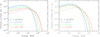 |
Fig. 1. Left: comparison of the bi-Maxwellian energy distributions with T∥ = 2 × 10⁶ K and T⊥ = 107 K (p = 1/5, blue), 2 × 10⁷ K (p = 1/10, green), and 4 × 10⁷ K (p = 1/20, red) with the Maxwellian distributions having the same mean energy of particles (dashed lines). Right: the same, but for the T∥/T⊥ case, T⊥ = 2 × 10⁶ K and T∥ = 107 K (p = 5, blue), 2 × 10⁷ K (p = 10, green), and 2 × 10⁷ K (p = 20, red) and the corresponding Maxwelian ones (dashed lines). |
The differences of the bi-Maxwellian distributions from the Maxwellian ones increase with an increase of deviations of p = T∥/T⊥ from 1 and they are higher for the case when the temperature along the magnetic field is higher than the perpendicular one (T∥ > T⊥). The bi-Maxwellian distributions have their peak shifted to lower energies when the number of low-energy particles is higher and also show a high-energy tail that is however not of a power-law nature. The κ-distributions show similar signatures although exact shapes are different. Therefore, we can expected similar effects on the spectra to those of κ-distributions.
3. Calculation of synthetic line spectra
To calculate line intensities, the ionization and excitation states must be determined. We assume that the bi-Maxwellian electron distributions are formed in the flaring plasma in the reconnection plasma outflow or in collapsing magnetic traps, where the anisotropic acceleration can be effective. The electron densities in such a plasma can be high, up to several times 1011 cm−3 (e.g., Milligan et al. 2012; Del Zanna & Woods 2013; Dzifčáková et al. 2018). Therefore we take the plasma density at locations with the bi-Maxwellian distributions as 5 × 1010 cm−3. In this case, the ionization equilibration times are below 1 s and times to reach excitation equilibrium are even shorter.
In the equilibrium state, the line emissivity, εij
is expressed by (5)
(5)
where h is the Planck constant, c is the speed of light, λij is the wavelength of the transition between atomic level i and j, Aij is the Einstein coefficient for spontaneous emission,  is the number of ions with the excited level i,
  is the abundance of +k-ionized ions relative to the total number of ions for element X, AX is the abundance of the element X relative to hydrogen, NH is the total number of hydrogen ions, and Ne is the electron density. The ratio
  is given by the ionization equilibrium and
  is obtained from the excitation equilibrium. For the known emissivity, the line intensity is its integral along line of sight in the optically thin flare plasma.
In the flare conditions, the direct ionization, autoionization, and radiative and dielectronic recombination are important in the calculation of the ionization equilibrium. For any energy distribution function, the rate of an elementary process can be expressed as (6)
(6)
where σ is the cross section. For the numerical calculation of the ionization rates we used the ionization cross sections of Dere (2007). The total ionization rates are shown in the upper part of Fig. 2.
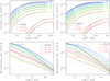 |
Fig. 2. The Fe ionization (upper) and recombination rates (bottom) for the bi-Maxwellian distribution with p = 1/5 (colored dot-dot-dot-dashed lines), 1/10 (color dashed lines), and 1/20 (colored full lines), (left), and p = 5 (colored dot-dot-dot-dashed lines), 10 (colored dashed lines), and 20 (colored full lines), (right) together with Maxwellian rates (black lines). Different colors correspond to different Fe ions. |
For the calculations of non-Maxwellian radiative recombination rates, the following relation for the radiative cross-sections was taken (e.g., Osterbrock 1974): (7)
(7)
where CRR is a constant and η + 0.5 is the power-law index, which can be found, for example, in Aldrovandi & Pequignot (1973) Landini & Monsignori Fossi (1990), Shull & van Steenberg (1982), Mazzotta et al. (1998), or Badnell (2006). The radiative recombination rates were integrated numerically.
For any distribution function, dielectronic recombination rates can be expressed as (Dzifčáková 1992; Dzifčáková & Dudík 2013) (8)
(8)
where cm and Em are the parameters from the approximations of the Maxwellian dielectronic recombination rates. We used data from Abdel-Naby et al. (2012), Altun et al. (2004, 2006, 2007), Badnell (2006), Bautista & Badnell (2007), Colgan et al. (2003, 2004), Mitnik & Badnell (2004), and Zatsarinny et al. (2004, 2005a,b, 2006). These data are freely available in the CHIANTI database (Dere et al. 2009). The total recombination rates are shown at the bottom of Fig. 2 and the effect of the bi-Maxwellian distributions on the ionization equilibrium is shown in Fig. 3.
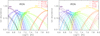 |
Fig. 3. The Fe ionization equilibrium for the Maxwellian distribution (full lines), bi-Maxwellian electron distributions with p = 1/5 (dot-dot-dot-dashed lines), 1/10 (dashed lines), and 1/20 (dot-dashed lines), (left), p = 5 (dot-dot-dot-dashed lines), 10 (dashed lines), and 20 (dot-dashed lines), (right). Different colors correspond to different Fe ions, see numbers. |
More details about the method for the calculation of the nonMaxwellian ionization and recombination rates can be found in Dzifčáková (1992), Dzifčáková & Dudík (2013), and Dzifčáková et al. (2017), for example.
The electron collisional excitation and de-excitation together with the spontaneous radiative decay transitions must be considered in the calculation of the excitation equilibrium. The collisional excitation and de-excitation are affected by the electron distribution. The excitation (de-excitation) rate can be calculated as (9)
(9)
where σij is the excitation cross-section for the transition from level i to level j, Ei is the energy of the incident electrons and f(Ei) is their energy distribution, ωi is the statistical weight of the level i, a0 is the Bohr radius, and Ωij is the collision strengths commonly used for the calculations of the electron excitation rates.
The majority of databases including the CHIANTI database (Dere et al. 1997; Del Zanna et al. 2015) contain the Maxwellian-averaged collision strengths only. The huge data volumes of original Ωs result in their unavailability. Therefore, the method for the approximation of Ωs from their integrals over the Maxwellian distribution was developed and tested by Dzifčáková & Mason (2008) and Dzifčáková et al. (2015), for example. The Ω approximations were used in the KAPPA package for the calculations of the synthetic spectra for the κ-distributions (Dzifčáková et al. 2015). The freely available KAPPA package contains Ω integrated over κ-distributions only to reduce time requirements for the calculations of the synthetic spectra. However, we still have a database of the Ω approximations. Slightly modified KAPPA software was used with our procedure for the numerical integration of Ω approximations for Fe XVII - Fe XXIV over bi-Maxwellian distributions to calculate the corresponding excitation rates.
The Ω approximations were obtained from the atomic data by Badnell & Griffin (2001), Badnell et al. (2001), Bautista et al. (2003, 2004), Berrington & Tully (1997), Brown et al. (2002), Butler & Zeippen (2001), Chidichimo et al. (2005), Del Zanna & Mason (2005), Del Zanna et al. (2005), Del Zanna (2006), Drake (1986), Edlén (1984), Fawcett et al. (1987), Feldman et al. (2000), Gu (2003), Kucera et al. (2000), Landi & Phillips (2005), Landi & Gu (2006), Palmeri et al. (2003), Sampson et al. (1983), Whiteford et al. (2001, 2002), and Witthoeft et al. (2006, 2007). These data are included in the CHIANTI database (Dere et al. 1997; Del Zanna et al. 2015).
4. Results and discussion
In agreement with the results of Paesold & Benz (1999, 2003), we assume that the continuous acceleration in the cascading magnetohydrodynamic turbulence in the reconnection plasma outflow generates the bi-Maxwellian distribution with the ratio p = T∥/T⊥ up to 20. In this case it is expected that the acceleration of electrons is faster than their isotropization. The characteristic isotropization time can be expressed as (Benz 1993) (10)
(10)
where υtest is the test particle velocity that in our case is about the thermal electron velocity. For the parameters considered in our paper (e.g., for the plasma density 5 × 1010 cm−3 and temperature up to 40 MK) this time is about 0.01 s. We note that this time is proportional to the third power of the test particle velocity. For other possible acceleration processes like shock and direct electric field accelerations, see Paesold & Benz (1999).
For generation of the bi-Maxwellian distribution with T∥ < T⊥ , the betatron acceleration in the collapsing magnetic trap can be assumed. However, a trap collapse to high values of the magnetic field during the estimated isotropization time td is not very probable. Specifically, the collapse time corresponds to magnetohydrodynamic times, therefore a high compression in short isotropization time is possible only in small traps, which limits its observability. Nevertheless, we made computations not only in a broad range of the parameter p > 1, but also in a broad range of the parameter 1/p = T⊥/T∥ in order to show that the spectroscopic effects of the bi-Maxwellian distribution with T∥ < T⊥ is much smaller than those for the bi-Maxwellian distribution with T∥ > T⊥.
Moreover, the bi-Maxwellian distributions are considered to be an approximation of real distributions. Therefore, at high electron energies, that are important for spectroscopic effects, the distributions can be closer to the bi-Maxwellian distributions than at lower energies.
Considering these bi-Maxwellian distributions, we calculated equilibrium spectra under an assumption of the ionization and excitation equilibrium in the temperature range typical for solar flares, log(T/K)=6.9 − 7.5.
4.1. Ionization equilibrium
Fig. 2 shows the comparison of the ionization and recombination rates for the bi-Maxwellian distribution with the Maxwellian ones. The temperatures corresponds to the temperature of the bi-Maxwellian distribution calculated from the mean energy of electrons (Eq. (4)).
For both cases, the ionization rates for the bi-Maxwellian electron distributions are enhanced for lower temperatures and reduced for higher temperatures. These changes increase with the increasing difference p from 1. The effects on the ionization rates are larger for the cases with T∥ > T⊥ (p > 1). The recombination rates are typically enhanced although the real behavior depends on the relative contributions of the radiative and dielectronic recombination rates. This enhancement increases with a deviation of p from 1 and again it is higher f for the cases with T∥ > T⊥ (Fig. 2, left).
The ionization equilibria for the bi-Maxwellian distributions are shown in Fig. 3. A comparison with the ionization equilibrium for the Maxwellian distribution is also presented there. It can be seen here that the ionization peaks for the bi-Maxwellian distributions are wider and shifted typically to higher temperatures. Again, changes in the ionization equilibrium increase with increasing differences of p from 1 and they are more pronounced for the cases with T∥ > T⊥ (p > 1).
The shape of the bi-Maxwellian energy distribution is similar to the shape of the non-thermal κ-distribution (e.g., Dzifčáková 1992; Dzifčáková & Dudík 2013; Livadiotis 2015). The κ-distribution also has its maximum shifted to lower energy and shows an enhanced number of particles in the high-energy tail in comparison with the Maxwellian energy distribution. The shape of the κ-distribution is modeled by a free parameter κ. Lower values of κ mean a stronger deviation of the κ-distribution from the Maxwellian one. The κ-distribution becomes Maxwellian for κ → ∞. Figure 4 upper left compares the shape of the bi-Maxwellian distributions with κ-distributions. We show the comparison for bi-Maxwellian distributions with p > 1 only because of their stronger effect on the distribution shape and ionization equilibrium. The high-energy tails of these two distributions are different. The bi-Maxwellian distributions show an exponential decrease with the energy in their high-energy parts. The κ-distributions have a power-law tail with the power-law index κ + 0.5. lower power-law index with lower κ corresponds a higher number of particles in the high-energy tail of distribution. However, low-energy parts of the both distributions can be approximated by a Maxwelian.
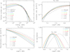 |
Fig. 4. Comparison of electron distributions (upper left), Fe XXI ionization (upper right ), recombination rate (bottom left), and ion abundance (bottom right) for the bi-Maxwellian distribution (p = 5 (blue lines), p = 10 (green line), p = 20 (red lines)), κ-distributions (κ = 5 (dot-dashed black line), κ = 3 (dashed black line), κ = 2 (dot-dot-dot-dashed black line)), and Maxwellian distribution (full black line). |
The behavior of the ionization rates reflects the shapes of distributions. Their decrease for higher temperatures is more significant for the κ-distributions than for the bi-Maxwellian distribution (Fig. 4, upper right). This is a result of the different shape of the high-energy tail.
The recombination rates for the bi-Maxwellian distributions change in a similar manner to the recombination rates for the κ-distribution (Fig. 4, bottom left). For example, the increase of the recombination rate for the bi-Maxwellian distribution with p = 20 is nearly the same as the increase for the κ-distribution with κ = 3 for the temperature corresponding to the Fe XXI abundance maximum.
The bottom-right panel of Fig. 4 shows that the abundance peaks for both the nonthermal distributions are wider in comparison with the Maxwellian one. This widening increases with the increase of the deviation of distributions from the Maxwellian one. The abundance peaks are also shifted to higher temperatures, however, the shift for the κ-distributions is much more significant. This is mainly due to the behavior of their ionization rates. The similarities in the changes in the ionization equilibrium for both distributions show that we can expect similar changes in the ionization equilibrium for any kind of distribution with an enhanced number of particles in the high-energy tail. However, the nature of the changes and their magnitudes depend on the nature of the distribution function.
4.2. Line intensities
The equilibrium EUV line synthetic spectra of iron for the bi-Maxwellian distributions were calculated for p = 1/5, 1/10, and 1/20 and for p = 5, 10, and 20, the spectral bands of SDO/EVE spectrograph 70–600 Å the temperature range log(T/K)=6.9 − 7.5, and electron density Ne = 5 × 1010 cm−3. The spectral, temperature, and density ranges were adopted according to Dzifčáková et al. (2018) to compare effects of the bi-Maxwellian distribution on the flare spectra with the effects of κ-distribution.
We first analyzed the effect of the bi-Maxwellian distributions on the temperature diagnostics. To diagnose flare temperatures from EVE data, the line ratios of Fe XXII 135.8 Å/Fe XX 121.8 Å or Fe XXIV 192.0 Å/Fe XXII 135.8 Å were used (e.g., Del Zanna & Woods 2013). Figure 5 shows a comparison of temperature dependence of these line ratios for different values of p. With increasing deviation of p from 1, the slope of lines becomes shallower. This results in differences for diagnosed temperatures; for example the observed value of the line ratio Fe XXIV 192.0 Å/Fe XXII 135.8 Å = 0.3 corresponds to the log(T/K)≈7.3 in the extreme case of the bi-Maxellian distribution with p = T∥/T⊥ = 20 but to the log(T/K)≈7.2 under the assumption of a Maxwellian distribution. This temperature difference increases with diagnosed temperature. For the known energy distribution, the temperature diagnostics from the line ratios of ions in different ionization degrees shows relatively high precision. The reasons for this are two. Firstly, strong lines used for diagnostics usually have very good photon statistics and their uncertainties are only slightly higher than the calibration uncertainties of EUV spectrographs (typically 20%). Secondly, the line ratios change very steeply with temperature, so the final error in the determination of Log(T) can be very small, Δ(Log(T/K)) ≈ 0.03, which is smaller than differences due to the shape of the energy distribution.
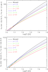 |
Fig. 5. The ratio of Fe XXII 135.8 Å/Fe XX 121.8 Å (upper) and Fe XXIV 192.0 Å/Fe XXII 135.8 Å (bottom) as a function of temperature for the Maxwellian distribution (black full line) and different bi-Maxwellian distributions with p = 1/5 (blue dashed lines), 1/10 (green dashed lines), 1/20 (red dashed lines), and p = 5 (blue full lines), 10 (green full lines), and 20 (red full lines). |
The temperature diagnostics for the κ-distributions show similar behavior to bi-Maxwellian ones (Dzifčáková et al. 2018). However, differences in the diagnosed temperatures are much higher for the κ-distributions than for the bi-Maxwellian ones (Fig. 6). This is the result of different shifts of the abundance peaks for these distributions.
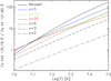 |
Fig. 6. The temperature dependence of the Fe XXII 135.8 Å/Fe XX 121.8 Å ratio for the Maxwellian distribution (black full line), bi-Maxwellian distributions with p = 5 (blue full line), 10 (green full line), and 20 (red full line), and for the κ-distributions with κ = 5 (dot-dashed black line), 3 (dashed black line), and 2 (dot-dot-dot-dashed black line). |
4.3. Distribution diagnostics
We need to diagnose parameter p and temperature simultaneously. Therefore we have to use at least two line ratios for a diagnostic of the non-Maxwellian distribution (Dzifčáková & Kulinová 2010; Mackovjak et al. 2013; Dudík et al. 2015). To propose the diagnostics of the parameter p for the bi-Maxwellian distributions we employed the same line ratios as in Dzifčáková et al. (2018) for the κ-distributions. The resulting ratio–ratio diagrams for Fe XXII, Fe XXI (upper), and for Fe XVIII, Fe XIX, Fe XX (bottom) are shown in Fig. 7. Similarly to the previous cases, with the increasing deviation of p from 1, the shift of the corresponding line ratios increases and becomes more significant for p > 1. This shift can be about 20% for the extreme case p = T∥/T⊥ = 20. The lines corresponding to the bi-Maxwellian distributions are shifted from the Maxwellian line in the same direction regardless of whether p < 1 or p > 1.
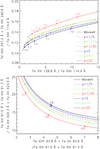 |
Fig. 7. Diagnostics of the parameter p of bi-Maxwellian distributions from line ratios of Fe XXII an Fe XXI (upper) and from line ratios of Fe XVIII, Fe XIX and Fe XX (bottom). The line coding is the same as in Fig. 5. Labels mark points corresponding to log(T) for the Maxwellian distribution (black) and bi-Maxwellian distribution with p = 20 (red). Numbers correspond to the Log(T). |
We also compared the diagnostic diagram for the bi-Maxwellian distributions for p > 1 with the diagnostics diagram for the κ-distributions (Fig. 8). The changes in the line ratios for the κ-distributions are similar to the changes for the bi-Maxwellian distributions and the line ratios for p = 20 correspond to the κ-distribution with κ ≈ 2.5. However, the same line ratios correspond to the different temperatures in the different nonthermal distributions. The temperatures for the κ-distributions are approximately 1.6× higher than for the bi-Maxwellian ones. This is the result of different shifts of the abundance maxima for the κ-distributions and bi-Maxwellian ones. This means that the diagnosed temperature depends on the nature of the distribution.
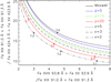 |
Fig. 8. The comparison of diagnostic ratio–ratio diagrams for the bi-Maxellian distribution with p = 5 (green line), 10 (blue line), 20 (red line) with the diagnostic ratio–ratio diagrams for the κ-distributions with κ = 5 (dot-dashed black line), 3 (dashed black line), and 2 (dot-dot-dot-dashed black line). Numbers correspond to the Log(T). |
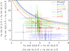 |
Fig. 9. As in Fig. 7 (bottom) but with the observed line ratios from SDO/EVE X-class flare analyzed by Dzifčáková et al. (2018). Increasing time of the observation corresponds to color changes black-bluegreen-yellow-orange-red of observed ratios with their error bars. |
Finally, the observed line ratios from the EVE 5.4X-class flare on 2012 March 7 00:02-00:24-00:40 UT (Dzifčáková et al. 2018) were added to the ratio-ratio diagram for Fe XVIII, Fe XIX, Fe XX for the illustration and comparison with real observations. The nonthermal effects in the spectrum of this flare have been analyzed by Dzifčáková et al. (2018). There one minute averaged line intensities from 00:07 UT to 00:50 UT were used for the nonthermal diagnostics. The observed line ratios show relatively high errors because of the lower photon statistics of the used lines. Therefore, for the estimation of the energy distribution it is better to use the distribution diagnostics. For the improvement of the temperature diagnostics, the line ratios of the ions at different degrees of ionization can be used.
Observed line ratios with their error bars shown in black or blue colors correspond to the impulsive phase and flare peak (00:07–00:25 UT). Green, yellow, and red colors of the line ratios correspond to the gradual phase of the flare (00:26–00:50 UT). Observed line ratios are shifted from the Maxwellian ratios in the same direction as the theoretical ratios for the bi-Maxwellian distributions. However, observed line ratios during the impulsive phase of the flare correspond to p higher than 20 if we want to interpret them under the assumption of the bi-Maxwellian distribution. Such a high value of p seems to be extreme.
5. Conclusions
We analyzed the effects of the bi-Maxwellian electron distribution on the ionization and excitation equilibrium with consequences on the temperature diagnostics of the flare plasma. Possible diagnostics of the bi-Maxwellian electron distributions were shown. The results were compared with the results for the κ-distributions.
Our analysis shows that the anisotropic bi-Maxwellian velocity distributions transform into nonthermal energy distributions with a high-energy tail and their maximum shifted to lower energies in comparison to the Maxwellian ones. With an increase of the deviation of p = T∥/T⊥ from 1, the changes in the shape of the bi-Maxwellian distributions, ionization equilibrium, and relative line intensities also increase. This affects the temperature diagnostics of plasma and gives us the possibility to diagnose the parameter p and therefore the shape of the energy distribution of particles.
The effects are more significant for the bi-Maxwellian distribution with T∥ > T⊥. The reason is that the bi-Maxwellian distribution with p > 1 has a more beam-like character than that with p < 1. Moreover, considering different acceleration mechanisms and collisional isotropization we think that the bi-Maxwellian distributions with high deviations from the Maxwellian one are more probable for those with p > 1 than for those with p < 1. Therefore, distributions with p > 1 can be much more readily diagnosed.
The energy distributions with the same significant attributes (e.g., presence of the high-energy tail) have similar effects on the temperature diagnostics and ratio–ratio diagrams used for diagnostics of a distribution function, although diagnosed temperature depends on the assumed distribution function. In this sense, at the present state of spectral diagnostics it is difficult to distinguish between the bi-Maxwellian and κ-distribution from line ratios alone. The effect of the bi-Maxwellian distribution with T∥/T⊥ = 20 on the line ratios is comparable with the effect of the strongly nonthermal κ-distribution with κ ≈ 2.5 (Fig. 8). From this comparison it appears that κ-distributions are able to produce line ratios closer to the strongly non-Maxwellian ratios that are observed during the impulsive flare phase than the bi-Maxwellian ones.
An important consequence of our calculations is that similar types of nonthermal energy distributions with high-energy tails have similar effects on the relative EUV spectral line intensities and temperature diagnostics. Therefore, the diagnostic diagram allows us to diagnose the presence of high-energy particles regardless of the shape of the high-energy tail. The comparison of the observed line ratios with theoretical calculations shows that strongly nonthermal distributions with the strong high-energy tails are present during the impulsive phase of the flares.
Finally, we must note that at present there is no possibility to diagnose the shape of the electron distribution in the velocity space from EUV spectra. Therefore, we are not able to distinguish between the effects of isotropic and anisotropic velocity distributions. Perhaps coordinated co-spatial observations in different spectral ranges (radio, X-ray) together with measurements of their polarization could help us to solve this problem.
Acknowledgments
We thank the anonymous referee for valuable comments. We acknowledge support from Grants 18-09072S, 17-16447S, and 16-13277S by the Grant Agency of the Czech Republic and from the AV ČR grant RVO:67985815.
References
- Abdel-Naby, S. A., Nikolić, D., Gorczyca, T. W., Korista, K. T., & Badnell, N. R. 2012, A&A, 537, A40 [NASA ADS] [CrossRef] [EDP Sciences] [Google Scholar]
- Aldrovandi, S. M. V., & Pequignot, D. 1973, A&A, 25, 137 [NASA ADS] [Google Scholar]
- Altun, Z., Yumak, A., Badnell, N. R., Colgan, J., & Pindzola, M. S. 2004, A&A, 420, 775 [NASA ADS] [CrossRef] [EDP Sciences] [Google Scholar]
- Altun, Z., Yumak, A., Badnell, N. R., Loch, S. D., & Pindzola, M. S. 2006, A&A, 447, 1165 [NASA ADS] [CrossRef] [EDP Sciences] [Google Scholar]
- Altun, Z., Yumak, A., Yavuz, I., et al. 2007, A&A, 474, 1051 [NASA ADS] [CrossRef] [EDP Sciences] [Google Scholar]
- Badnell, N. R. 2006, A&A, 447, 389 [NASA ADS] [CrossRef] [EDP Sciences] [Google Scholar]
- Badnell, N. R., & Griffin, D. C. 2001, J. Phys. B At. Mol. Phys., 34, 681 [NASA ADS] [CrossRef] [Google Scholar]
- Badnell, N. R., Griffin, D. C., & Mitnik, D. M. 2001, J. Phys. B At. Mol. Phys., 34, 5071 [NASA ADS] [CrossRef] [Google Scholar]
- Bautista, M. A., & Badnell, N. R. 2007, A&A, 466, 755 [NASA ADS] [CrossRef] [EDP Sciences] [Google Scholar]
- Bautista, M. A., Mendoza, C., Kallman, T. R., & Palmeri, P. 2003, A&A, 403, 339 [NASA ADS] [CrossRef] [EDP Sciences] [Google Scholar]
- Bautista, M. A., Mendoza, C., Kallman, T. R., & Palmeri, P. 2004, A&A, 418, 1171 [NASA ADS] [CrossRef] [EDP Sciences] [Google Scholar]
- Benz, A. O., 1993, in Plasma Astrophysics: Kinetic Processes in Solar and Stellar Coronae, Astrophysics and Space Science Library, 184, 47 [NASA ADS] [Google Scholar]
- Berrington, K. A., & Tully, J. A. 1997, A&AS, 126, [Google Scholar]
- Bian, N. H., Emslie, A. G., Stackhouse, D. J., & Kontar, E. P. 2014, ApJ, 796, 142 [NASA ADS] [CrossRef] [Google Scholar]
- Bingham, R., Dawson, J. M., & Shapiro, V. D. 2002, J. Plasma Phys., 68, 161 [NASA ADS] [CrossRef] [Google Scholar]
- Brown, J. C. 1971, Sol. Phys., 18, 489 [NASA ADS] [CrossRef] [Google Scholar]
- Brown, G. V., Beiersdorfer, P., Liedahl, D. A., et al. 2002, ApJS, 140, 589 [NASA ADS] [CrossRef] [Google Scholar]
- Butler, K., & Zeippen, C. J. 2001, A&A, 372, 1083 [NASA ADS] [CrossRef] [EDP Sciences] [Google Scholar]
- Chidichimo, M. C., Del Zanna, G., Mason, H. E., et al. 2005, A&A, 430, 331 [NASA ADS] [CrossRef] [EDP Sciences] [Google Scholar]
- Colgan, J., Pindzola, M. S., Whiteford, A. D., & Badnell, N. R. 2003, A&A, 412, 597 [NASA ADS] [CrossRef] [EDP Sciences] [Google Scholar]
- Colgan, J., Pindzola, M. S., & Badnell, N. R. 2004, A&A, 417, 1183 [NASA ADS] [CrossRef] [EDP Sciences] [Google Scholar]
- Del Zanna, G. 2006, A&A, 459, 307 [NASA ADS] [CrossRef] [EDP Sciences] [Google Scholar]
- Del Zanna, G., & Mason, H. E. 2005, A&A, 433, 731 [NASA ADS] [CrossRef] [EDP Sciences] [Google Scholar]
- Del Zanna, G., & Woods, T. N. 2013, A&A, 555, A59 [NASA ADS] [CrossRef] [EDP Sciences] [Google Scholar]
- Del Zanna, G., Chidichimo, M. C., & Mason, H. E. 2005, A&A, 432, 1137 [NASA ADS] [CrossRef] [EDP Sciences] [Google Scholar]
- Del Zanna, G., Dere, K. P., Young, P. R., Landi, E., & Mason, H. E. 2015, A&A, 582, A56 [NASA ADS] [CrossRef] [EDP Sciences] [Google Scholar]
- Dere, K. P. 2007, A&A, 466, 771 [NASA ADS] [CrossRef] [EDP Sciences] [Google Scholar]
- Dere, K.P., Landi, E., Mason, H. E., Monsignori Fossi, B. C., & Young, P. R. 1997, A&AS, 125, 149 [NASA ADS] [CrossRef] [EDP Sciences] [Google Scholar]
- Dere, K. P., Landi, E., Young, P. R., et al. 2009, A&A, 498, 915 [NASA ADS] [CrossRef] [EDP Sciences] [Google Scholar]
- Drake, G. W. F. 1986, Phys. Rev. A, 34, 2871 [NASA ADS] [CrossRef] [PubMed] [Google Scholar]
- Dudík, J., Mackovjak, Š., Dzifčáková, E., et al. 2015, ApJ, 807, 123 [NASA ADS] [CrossRef] [Google Scholar]
- Dzifčáková, E. 1992, Sol. Phys., 140, 247 [NASA ADS] [CrossRef] [Google Scholar]
- Dzifčáková, E., & Dudík, J. 2013, ApJS, 206, 6 [NASA ADS] [CrossRef] [Google Scholar]
- Dzifčáková, E., & Kulinová, A. 2010, Sol. Phys., 263, 25 [NASA ADS] [CrossRef] [Google Scholar]
- Dzifčáková, E., & Mason, H. 2008, Sol. Phys., 247, 301 [NASA ADS] [CrossRef] [Google Scholar]
- Dzifčáková, E., Dudík, J., Kotrč, P., Fárník, F., & Zemanová, A. 2015, ApJS, 217, 14 [NASA ADS] [CrossRef] [Google Scholar]
- Dzifčáková, E., Vocks, C., & Dudík, J. 2017, A&A, 603, A14 [NASA ADS] [CrossRef] [EDP Sciences] [Google Scholar]
- Dzifčáková, E., Zemanová, A., Dudík, J., & Mackovjak, Š. 2018, ApJ, 853, 158 [NASA ADS] [CrossRef] [Google Scholar]
- Edlén, B. 1984, Phys. Scr., 30, 135 [NASA ADS] [CrossRef] [Google Scholar]
- Fawcett, B. C., Phillips, K. J. H., Jordan, C., & Lemen, J. R. 1987, MNRAS, 225, 1013 [NASA ADS] [CrossRef] [Google Scholar]
- Feldman, U., Curdt, W., Landi, E., & Wilhelm, K. 2000, ApJ, 544, 508 [NASA ADS] [CrossRef] [Google Scholar]
- Fletcher, L., Dennis, B. R., Hudson, H. S., et al. 2011, Space Sci. Rev., 159, 19 [NASA ADS] [CrossRef] [Google Scholar]
- Gu, M. F. 2003, ApJ, 582, 1241 [NASA ADS] [CrossRef] [Google Scholar]
- Karlický, M., & Kosugi, T. 2004, A&A, 419, 1159 [NASA ADS] [CrossRef] [EDP Sciences] [Google Scholar]
- Kašparová, J., & Karlický, M. 2009, A&A, 497, L13 [NASA ADS] [CrossRef] [EDP Sciences] [Google Scholar]
- Kontar, E. P., Brown, J. C., Emslie, A. G., et al. 2011, Space Sci. Rev., 279 [Google Scholar]
- Krucker, S., Battaglia, M., Cargill, P. J., et al. 2008, A&A Rev., 16, 155 [Google Scholar]
- Kucera, T. A., Feldman, U., Widing, K. G., & Curdt, W. 2000, ApJ, 538, 424 [NASA ADS] [CrossRef] [Google Scholar]
- Landi, E., & Gu, M. F. 2006, ApJ, 640, 1171 [NASA ADS] [CrossRef] [Google Scholar]
- Landi, E., & Phillips, K. J. H. 2005, ApJS, 160, 286 [NASA ADS] [CrossRef] [Google Scholar]
- Landini, M., & Monsignori Fossi, B. C. 1990, A&AS, 82, 229 [NASA ADS] [Google Scholar]
- Livadiotis, G. 2015, J. Geophys. Res. Space Phys., 120, 1607 [Google Scholar]
- Mackovjak, Š., Dzifčáková, E., & Dudík, J. 2013, Sol. Phys., 282, 263 [NASA ADS] [CrossRef] [Google Scholar]
- Mazzotta, P., Mazzitelli, G., Colafrancesco, S., & Vittorio, N. 1998, A&AS, 133, 403 [NASA ADS] [CrossRef] [EDP Sciences] [Google Scholar]
- Milligan, R. O., Kennedy, M. B., Mathioudakis, M., & Keenan, F. P. 2012, ApJ, 755, L16 [NASA ADS] [CrossRef] [Google Scholar]
- Mitnik, D. M., & Badnell, N. R. 2004, A&A, 425, 1153 [NASA ADS] [CrossRef] [EDP Sciences] [Google Scholar]
- Oka, M., Ishikawa, S., Saint-Hilaire, P., Krucker, S., & Lin, R. P. 2013, ApJ, 764, 6 [NASA ADS] [CrossRef] [Google Scholar]
- Oka, M., Krucker, S., Hudson, H. S., & Saint-Hilaire, P. 2015, ApJ, 799, 129 [NASA ADS] [CrossRef] [Google Scholar]
- Osterbrock, D. E. 1974, Research supported by the Research Corp., (San Francisco: W. H. Freeman and Co.) [Google Scholar]
- Owocki, S. P., & Scudder, J. D. 1983, ApJ, 270, 758 [NASA ADS] [CrossRef] [Google Scholar]
- Paesold, G., & Benz, A. O. 1999, A&A, 351, 741 [NASA ADS] [Google Scholar]
- Paesold, G., & Benz, A. O. 2003, A&A, 401, 711 [NASA ADS] [CrossRef] [EDP Sciences] [Google Scholar]
- Palmeri, P., Mendoza, C., Kallman, T. R., & Bautista, M. A. 2003, A&A, 403, 1175 [NASA ADS] [CrossRef] [EDP Sciences] [Google Scholar]
- Sampson, D. H., Goett, S. J., & Clark, R. E. H. 1983, At. Data Nucl. Data Tables, 29, 467 [NASA ADS] [CrossRef] [Google Scholar]
- Shull, J. M., & van Steenberg, M. 1982, ApJS, 48, 95 [NASA ADS] [CrossRef] [Google Scholar]
- Simões, P. J. A., Graham, D. R., & Fletcher, L. 2015, Sol. Phys., 290, 3573 [NASA ADS] [CrossRef] [Google Scholar]
- Štverák, Š., Trávníček, P., Maksimovic, M., et al. 2008, J. Geophys. Res. Space Phys., 113, A03103 [Google Scholar]
- Štverák, Š., Maksimovic, M., Trávníček, P. M., et al. 2009, J. Geophys. Res. Space Phys., 114, A05104 [Google Scholar]
- Veronig, A. M., Rybák, J., Gömöry, P., et al. 2010, ApJ, 719, 655 [NASA ADS] [CrossRef] [Google Scholar]
- Vocks, C., Salem, C., Lin, R. P., & Mann, G. 2005, ApJ, 627, 540 [NASA ADS] [CrossRef] [Google Scholar]
- Whiteford, A. D., Badnell, N. R., Ballance, C. P., et al. 2001, J. Phys. B At. Mol. Phys., 34, 3179 [NASA ADS] [CrossRef] [Google Scholar]
- Whiteford, A. D., Badnell, N. R., Ballance, C. P., et al. 2002, J. Phys. B At. Mol. Phys., 35, 3729 [NASA ADS] [CrossRef] [Google Scholar]
- Witthoeft, M. C., Badnell, N. R., del Zanna, G., Berrington, K. A., & Pelan, J. C. 2006, A&A, 446, 361 [NASA ADS] [CrossRef] [EDP Sciences] [Google Scholar]
- Witthoeft, M. C., Del Zanna, G., & Badnell, N. R. 2007, A&A, 466, 763 [NASA ADS] [CrossRef] [EDP Sciences] [Google Scholar]
- Zatsarinny, O., Gorczyca, T. W., Korista, K., Badnell, N. R., & Savin, D. W. 2004, A&A, 426, 699 [NASA ADS] [CrossRef] [EDP Sciences] [Google Scholar]
- Zatsarinny, O., Gorczyca, T. W., Korista, K. T., et al. 2005a, A&A, 438, 743 [NASA ADS] [CrossRef] [EDP Sciences] [Google Scholar]
- Zatsarinny, O., Gorczyca, T. W., Korista, K. T., et al. 2005b, A&A, 440, 1203 [NASA ADS] [CrossRef] [EDP Sciences] [Google Scholar]
- Zatsarinny, O., Gorczyca, T. W., Fu, J., et al. 2006, A&A, 447, 379 [NASA ADS] [CrossRef] [EDP Sciences] [Google Scholar]
- Zharkova, V. V., Arzner, K., Benz, A. O., et al. 2011, Space Sci. Rev., 156, [Google Scholar]
All Figures
|
Fig. 1. Left: comparison of the bi-Maxwellian energy distributions with T∥ = 2 × 10⁶ K and T⊥ = 107 K (p = 1/5, blue), 2 × 10⁷ K (p = 1/10, green), and 4 × 10⁷ K (p = 1/20, red) with the Maxwellian distributions having the same mean energy of particles (dashed lines). Right: the same, but for the T∥/T⊥ case, T⊥ = 2 × 10⁶ K and T∥ = 107 K (p = 5, blue), 2 × 10⁷ K (p = 10, green), and 2 × 10⁷ K (p = 20, red) and the corresponding Maxwelian ones (dashed lines). |
| In the text | |
|
Fig. 2. The Fe ionization (upper) and recombination rates (bottom) for the bi-Maxwellian distribution with p = 1/5 (colored dot-dot-dot-dashed lines), 1/10 (color dashed lines), and 1/20 (colored full lines), (left), and p = 5 (colored dot-dot-dot-dashed lines), 10 (colored dashed lines), and 20 (colored full lines), (right) together with Maxwellian rates (black lines). Different colors correspond to different Fe ions. |
| In the text | |
|
Fig. 3. The Fe ionization equilibrium for the Maxwellian distribution (full lines), bi-Maxwellian electron distributions with p = 1/5 (dot-dot-dot-dashed lines), 1/10 (dashed lines), and 1/20 (dot-dashed lines), (left), p = 5 (dot-dot-dot-dashed lines), 10 (dashed lines), and 20 (dot-dashed lines), (right). Different colors correspond to different Fe ions, see numbers. |
| In the text | |
|
Fig. 4. Comparison of electron distributions (upper left), Fe XXI ionization (upper right ), recombination rate (bottom left), and ion abundance (bottom right) for the bi-Maxwellian distribution (p = 5 (blue lines), p = 10 (green line), p = 20 (red lines)), κ-distributions (κ = 5 (dot-dashed black line), κ = 3 (dashed black line), κ = 2 (dot-dot-dot-dashed black line)), and Maxwellian distribution (full black line). |
| In the text | |
|
Fig. 5. The ratio of Fe XXII 135.8 Å/Fe XX 121.8 Å (upper) and Fe XXIV 192.0 Å/Fe XXII 135.8 Å (bottom) as a function of temperature for the Maxwellian distribution (black full line) and different bi-Maxwellian distributions with p = 1/5 (blue dashed lines), 1/10 (green dashed lines), 1/20 (red dashed lines), and p = 5 (blue full lines), 10 (green full lines), and 20 (red full lines). |
| In the text | |
|
Fig. 6. The temperature dependence of the Fe XXII 135.8 Å/Fe XX 121.8 Å ratio for the Maxwellian distribution (black full line), bi-Maxwellian distributions with p = 5 (blue full line), 10 (green full line), and 20 (red full line), and for the κ-distributions with κ = 5 (dot-dashed black line), 3 (dashed black line), and 2 (dot-dot-dot-dashed black line). |
| In the text | |
|
Fig. 7. Diagnostics of the parameter p of bi-Maxwellian distributions from line ratios of Fe XXII an Fe XXI (upper) and from line ratios of Fe XVIII, Fe XIX and Fe XX (bottom). The line coding is the same as in Fig. 5. Labels mark points corresponding to log(T) for the Maxwellian distribution (black) and bi-Maxwellian distribution with p = 20 (red). Numbers correspond to the Log(T). |
| In the text | |
|
Fig. 8. The comparison of diagnostic ratio–ratio diagrams for the bi-Maxellian distribution with p = 5 (green line), 10 (blue line), 20 (red line) with the diagnostic ratio–ratio diagrams for the κ-distributions with κ = 5 (dot-dashed black line), 3 (dashed black line), and 2 (dot-dot-dot-dashed black line). Numbers correspond to the Log(T). |
| In the text | |
|
Fig. 9. As in Fig. 7 (bottom) but with the observed line ratios from SDO/EVE X-class flare analyzed by Dzifčáková et al. (2018). Increasing time of the observation corresponds to color changes black-bluegreen-yellow-orange-red of observed ratios with their error bars. |
| In the text | |
Current usage metrics show cumulative count of Article Views (full-text article views including HTML views, PDF and ePub downloads, according to the available data) and Abstracts Views on Vision4Press platform.
Data correspond to usage on the plateform after 2015. The current usage metrics is available 48-96 hours after online publication and is updated daily on week days.
Initial download of the metrics may take a while.