| Issue |
A&A
Volume 618, October 2018
|
|
|---|---|---|
| Article Number | A71 | |
| Number of page(s) | 16 | |
| Section | Planets and planetary systems | |
| DOI | https://doi.org/10.1051/0004-6361/201832883 | |
| Published online | 15 October 2018 | |
The near-nucleus gas coma of comet 67P/Churyumov-Gerasimenko prior to the descent of the surface lander PHILAE
1
Laboratoire de Métérologie Dynamique, Université Pierre et Marie Curie,
4 Place Jussieu,
75252 Paris, France
e-mail: This email address is being protected from spambots. You need JavaScript enabled to view it.
2
Laboratoire Atmosphères Milieux, Observations Spatiales, CNRS/UVSQ,
11 Boulevard d’Alembert,
78280 Guyancourt, France
3
Federal State Unitary Enterprise Russian Federal Nuclear Center All-Russian Research Institute of Experimental Physics (FSUE RFNC-VNIIEF), Sarov,
Nizhny Novgorod Region,
607188, Russia
4
Physikalisches Institut, University of Bern,
3012 Bern, Switzerland
Received:
22
February
2018
Accepted:
23
June
2018
Abstract
Context. The European Space Agency (ESA) Rosetta mission was the most comprehensive study of a comet ever performed. In particular, the Rosetta orbiter, which carried many instruments for monitoring the evolution of the dusty gas emitted by the cometary nucleus, returned an enormous volume of observational data collected from the close vicinity of the nucleus of comet 67P/Churyumov-Gerasimenko.
Aims. Such data are expected to yield unique information on the physical processes of gas and dust emission, using current physical model fits to the data. We present such a model (the RZC model) and our procedure of adjustment of this model to the data.
Methods. The RZC model consists of two components: (1) a numerical three-dimensional time-dependent code solving the Eulerian/Navier-Stokes equations governing the gas outflow, and a direct simulation Monte Carlo (DSMC) gaskinetic code with the same objective; and (2) an iterative procedure to adjust the assumed model parameters to best-fit the observational data at all times.
Results. We demonstrate that our model is able to reproduce the overall features of the local neutral number density and composition measurements of Rosetta Orbiter Spectrometer for Ion and Neutral Analysis (ROSINA) Comet Pressure Sensor (COPS) and Double Focusing Mass Spectrometer (DFMS) instruments in the period August 1–November 30, 2014. The results of numerical simulations show that illumination conditions on the nucleus are the main driver for the gas activity of the comet. We present the distribution of surface inhomogeneity best-fitted to the ROSINA COPS and DFMS in situ measurements.
Key words: comets: individual: 67P/Churyumov-Gerasimenko / comets: general / methods: numerical / hydrodynamics
© ESO 2018
 Open Access article, published by EDP Sciences, under the terms of the Creative Commons Attribution License (http://creativecommons.org/licenses/by/4.0), which permits unrestricted use, distribution, and reproduction in any medium, provided the original work is properly cited.
1 Introduction
Several works have undertaken the derivation of the distribution of the surface activity of comet 67P/Churyumov-Gerasimenko (hereafter 67P) from the in situ measurements made near to the nucleus by the Rosetta Orbiter Spectrometer for Ion and Neutral Analysis (ROSINA) consisting of two mass spectrometers and a pressure sensor (Balsiger et al. 2007). This requires (1) the use of a coma gas model relating the gas flow variables at any point to a set of adjustable parameters meant to represent the nucleus surface gas production (i.e. defining the so-called flow “surface boundary conditions”), and (2) an iterative procedure to derive the best-fit values of these parameters.
The coma gas model has two requirements: (1) compliance with the well-established rules of physical gasdynamics and (2) plausibility of the surface boundary conditions including the complex shape of the nucleus and the associated intricate illumination conditions. The inhomogeneous gas flow in the coma is characterized by the juxtaposition of regions with different flow regimes from free-molecular to fluid, the presence of multiple shocks, and non-equilibrium. The universal approach to handle this situation is the direct simulation Monte Carlo (DSMC) kinetic method (Bird 1994), but this may become very expensive in terms of computational time and required memory space. However, as has been demonstrated in many previous works, inviscid and/or viscous fluid methods (e.g. Euler equations, EE, or Navier-Stokes equations, NSE) can describe the flow in the coma with sufficient precision while preserving a high computational efficiency (e.g. Lukyanov et al. 2005).
The second aspect (the relevance of boundary conditions) consists in the underlying physical model and the way parameters for this model were derived. Complex, precise physical model with multiple parameters may have no benefit owing to the large uncertainty in the parameters magnitudes due to the lack of precise observational information. The other limit – an oversimplified model – is not worth the effort since it has no physical meaning.
In Bieler et al. (2015), both kinetic and fluid approaches were used (we do not consider the third, purely geometrical model) to compute the gas flow, assuming a pure water production from a homogeneous surface. At each surface point the gas flux and the surface temperature varied between imposed minimum and maximum values according to the cosine of the local solar zenith angle (i.e. gas production and surface temperature are decoupled). This model was able to reproduce the overall features of the local neutral number density measurements for the time period between early August 2014 and January 1, 2015, although some details in the measurements were not reproduced. Also, it should be noted that additional latitude-dependent correction factors were applied in a post-processing manner to the model outputs to improve the correlation to the observations.
In Fougere et al. (2016a,b), the gas coma was simulated by the DSMC method and took into account the most abundant observed components: H2O and CO2 or H2O, CO2, CO, and O2, respectively. The model of activity was similar to Bieler et al. (2015) but with the addition of surface inhomogeneity factors (for each species) to each surface element. The heterogeneity pattern of the surface outgassing activity was constrained by in situ coma density and composition measurements performed from August 2014 to the end of February 2016. A formal numerical data inversion method based on the extension of the geometrical model from Bieler et al. (2015) was used for the derivation of the surface fluxes. Agreement of the adjusted model and measurements was quantified by the root mean square deviation normalized by the mean measured value (for H2O and CO2, these are 1.14 and1.08, respectively). It should be noted that (1) during a large part of this time period the Rosetta spacecraft was at distances greater than 100 km from the nucleus (where many flow structures are washed away) and (2) derivation of the surface properties based on long period measurements implicitly suggests that surface properties are invariable on this timescale (which is unlikely for more than one year).
In Marschall et al. (2016) the DSMC method was used assuming a pure H2O coma (though there is a high relative abundance of carbon dioxide in the ROSINA data set). The model of gas production assumed surface ice sublimation from an inhomogeneous surface. The distribution of surface inhomogeneity was postulated by a set of patches. The geometry of patches was inspired by the observed surface morphology (i.e. it is not connected explicitly with surface activity). Marschall et al. (2016) also investigated activity from cliffs versus plains, setting the difference between the two at a certain angle of the surface with respect to the local gravity field. The total number of defined regions on the surface of the nucleus is 26 and each is of a considerable size, therefore adjustment by patches is rather crude. The outgassing activity of patches at the surface was constrained by in situ coma density measurements performed from the end of August to the end of September 2014. It is worth noting that in this work simulation was done for the 10 km size region only. Beyond 10 km the simulated data were extrapolated assuming radial outflow with constant velocity.
In Kramer et al. (2017), a “simplified analytical model” (a kind of a collisionless expansion from point sources placed at shape model facets) was used for the definition of the gas coma parameters distribution. It is clear, however, that the gas coma was anything but collisionless. Furthermore, the model considered the time-averaged (over several weeks) surface emission rate and did not consider oscillations caused by momentary illumination conditions. The gas model of gas production was constructed by fitting tens of thousands of measurements to thousands of potential gas sources distributed across the entire nucleus surface. The relative difference with in situ density measurements was 11–18%.
It should be noted that the period of fitting was 2015–2016 and at this time Rosetta was at more than 100 km from the nucleus and therefore the numerous gas structures that are formed by collisions in the nucleus vicinity become in large part smoothed out. Therefore, the good agreement between an artificial collisionless model with quite homogeneous surface properties and smoothed-out structures are a natural consequence. However, the correlation to the footpoints of dust outbursts identified by the Optical, Spectroscopic, and Infrared Remote Imaging System (OSIRIS), even one year after the occurrence found in this work, is rather remarkable.
This short overview of currently published results on the distribution of surface activity shows that (1) the gas production mechanism is formulated in different ways; (2) the methods used to constrain the models are different; (3) the resulting patterns of surface activity are quite different and no one model fits perfectly the observational data for the close distances over a long period. Therefore, the derivation of surface activity still deserves attention.
In the present work we present in detail our own model and the results of its adjustment to the in situ measurements. We restrict ourselves to the so-called “prelanding data” collected in August–November 2014, which we had to interpret in real time to predict the aerodynamic force exerted on the lander during its descent (Jurado et al. 2016). We use both fluid and kinetic methods alternately in order to reduce computational expenses but keep the physical accuracy. The method based on fluid approach uses Euler equations and was described in Rodionov et al. (2002). The kinetic approach was implemented on the basis of the DSMC method. The same methods are used in the fitting procedure.
2 RZC model description
The observational nucleus data for the model were (a) a nucleus rotation model, and (b) a nucleus surface shape model. To these we added our coma gas flow model(s) and our surface production model.
2.1 Nucleus surface model
Many variants of the nucleus shape model were derived during the mission. In the present work we adopted the so-called “RMOC shape 3” (see Fig. 1), despite the fact that there are more precise shape models of 67P at the present time. This was done for the following reasons: (1) we started our work in 2014 and at that time it was the most precise model; (2) we study the period August–November 2014 when the Sun was in the northern hemisphere and the northern part of the shape was mapped with sufficient precision; (3) the more precise model would have needed to be degraded anyway in order to reduce the number of surface elements to match the requirements of the gas outflow solvers.
2.2 Nucleus rotation model
From the orbiter camera images, the nucleus rotation was accurately determined as a single-axis rotation with constant period (12.40 h) and invariant axis (OZ in the present figures) inclined in the period under discussion from 45° to 55° from the Sun direction.
2.3 Structure of the gas coma computational grid
This model is given as an unstructured triangular grid with a resolution of about 30 metres. In our computations we use a block-structured grid consisting of six blocks joined in a “football” manner (see Fig. 2 of this paper and Rodionov & Crifo (2006) for more details) and this grid covers the whole surface. Since the shape model is non-stellar-like, the grid generation procedure used in Rodionov & Crifo (2006) was modified. In the present version the initial point for radial directions is floating along the X-axis between −1 and 2 in order to ensure that the radial direction from the initial point crosses the surface only once. In addition, the resolution of the shapemodel is excessively fine for gas outflow simulations. Therefore, for computations we generated three versions Si of an “effective surface model” to be used by the gas code differing by the characteristic angular resolution of cells (1o × 1o, 2.5o × 2.5o and 5o × 5o). This procedure evidently erases all small-scale details (see images in Fig. 1) but also creates a surface slightly different from the “real” one, which has, for example, a different shadow pattern under oblique solar illumination. Figure 1 shows a comparison of the initial shapemodel with the “effective surface model” of different resolution. The volume grid is constructed having the effective surface model as the inner boundary (ground level) and a sphere as the outer boundary (top level, see Fig. 2). The radial spacing of levels is non-uniform to ensure that the radial steps near the surface and near the outer boundary are comparable with inner and outer surface cell resolution, respectively. The model allows for the rotation by a succession of steady-state solutions separated by a constant time interval δt such that (1) during δt the computed surface temperatures and gas fluxes vary negligibly, and (2) the typical gas transit time across the computational domain is smaller thanδt.
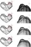 |
Fig. 1 Shape models: RMOC shape 3 (first row) and effective surface model with resolution 1o × 1o (second row), 2.5o × 2.5o (third row), 5o × 5o (bottom row). Left column: view (from −Y) on the full shape. Right column: scaled-up part from the red box (with a surface grid shown in black). |
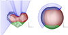 |
Fig. 2 Example of the computational grid: near the surface (left panel) and close to the outer boundary (right panel). The blocs comprising the “football” grid are shown in different color. |
2.4 Nucleus gas production model
From Earth-based observations of comets, yielding (1) an approximate global production rate Qi of the most abundantly produced molecules and (2) a coarse image of the resulting dusty atmosphere – the so-called “coma” – it has long since been considered that the less volatile molecules (e.g. H2O) are produced from the surface of the nucleus by sublimation of (sub)surface ice inclusions and that the more volatile molecules are produced bydiffusion through the surface after having been sublimated at variable depths inside the nucleus. It follows that the H2O emission must peak at sunlit points, while that of the other molecules need not be limited to such points and could even be nearly uniformly produced over the surface if deep production is involved. Thus, due to the nucleus rotation, the coma is expected to have two time-dependent components: one confined to the sunward hemisphere and the other co-rotating with the nucleus.
Considering the fact that inside each surface grid element there may be a complex topography and therefore temperature inhomogeneity, the distribution of ice may assume any pattern, and the CO and CO2 production may also have stochastic variations, it was considered simply impossible to perform a gas-dynamically exact modelling of the near-surface non-equilibrium outflow region. Instead, our treatment was a trivial extension of that used in Rodionov et al. (2002) where stochastic fluctuations are absent:
- (1)
The initial gas parameters T0, P0 were related to the initial equilibrium flow Mach number M0 by the plane-parallel homogeneous vapour sublimation relations derived by Cercignani (1981).
- (2)
Whether condensation or sublimation of H2O occurred was selected by the Riemann problem solution of the fluid EE or NSE, which also provided M0.
In the absence of reliable information on the interior of the comet nucleus surface, the number of parameters to introduce for a proper representation of the gas production is potentially very large. However, based on our in-depth analysis of the 1986 Halley comet fly-by data (Szegö et al. 2002), we used a minimal number of parameters. For H2O we assume that each elementary surface area contains some fraction  of exposed ice (≤1 and it should also be noted that since no large patches of ice were observed on the surface, this factor might be quite small). The upward H2O flux is therefore equal to
  where FHK is the ice Hertz–Knudsen sublimation rate, and Tn is the surface ice temperature, computed from a slightly modified classical sunlit ice energy budget equation:
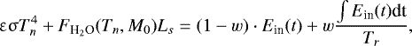 (1)
(1)
where  is the net sublimating gas flux, M0 is the initial gas Mach number, LS is the latent heat of sublimation, ε is the surface infrared emissivity, σ is the Boltzmann constant, Ein is incoming energy at instant t, w is a proportion of instantaneous and rotation averaged energy input, and Tr is the period of rotation. The rotation-averaged term allows us to also consider the time lag of the heat transfer. The case in which w = 0 corresponds to an instantaneous adjustment of the surface temperature to the illumination (i.e. high thermal conductivity). The case in which w = 1 corresponds to the case when the thermal state is defined by the mean illumination (low thermal conductivity),
 (2)
(2)
where AV is the dirty ice visible albedo, z⊙ is the solar zenith angle, c⊙ is the solar flux, and κ is an heuristic dimensionless model parameter representing a heat input from the nucleus interior. Figure 3 shows an example of the input energy distribution over the surface in two limiting cases: purely instantaneous and rotation-averaged. The presence of shadowing of one element by the nucleus orography is taken into account by a ray-tracing method (without regard for reradiation). Let us stress that, at any point, H2O sublimation or condensation may occur, depending upon the surrounding conditions.
For CO and CO2 we adopt total production rates QCO and  and assume that the fluxes FCO and
  are distributed over the surface according tolaws of the kind F = a + b max[cosz⊙, 0] where a and b are free parameters:
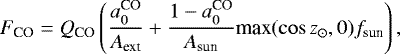 (3)
(3)
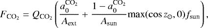 (4)
(4)
where Aext is the total surface area, Asun is the sunlit cross-section, a0 is the fraction of gas production distributed uniformly over the surface, and fsun is a shadow step function equal to 0 in shadow and to 1 otherwise.
For CO and CO2, we also attribute to each elementary surface area two factors, fCO and  , which affect the upward CO and CO2 fluxes in the following way: fCOFCO and
  . The physical nature of these factors is different from the fraction of exposed ice
  and they could vary from 0 to greater than 1. For example, these factors could be interpreted as an effect of the insulating dust layer thickness over the surface. When fCO > 1 or
  , it means that the corresponding total production rate QCO or
  was underestimated. In order to have fCO ≤ 1 and
  , the imposed total production rates should be multiplied by the peak values
  and
and  and at the same time the inhomogeneity factors of surface elements should be divided by these peak values. In the following, we will refer to
  ,
,  and fCO as “the factors of surface inhomogeneity”. Figure 4 shows an example of the computed surface temperature for an icy and non-icy surface (for homogeneous surface, i.e. with constant
  , fCO, and
  ), for one orientation of the nucleus.
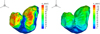 |
Fig. 3 Input energy distribution in the case of instantaneous energy input (left panel) and rotation averaged energy input (right panel). Computations made for Oct. 1, 2014, 07:08:00 UTC, the Sun being nearly in the plane Y = 0 and at 40° from +X. |
2.5 Gas outflow model
The approach we used is similar to that described in detail in Rodionov et al. (2002). However, special efforts had to be made to meet three essential constraints: (1) provide temporal and spatial resolutions comparable to those of the observations; (2) handle the coexistence in the computational domain of widely different rarefaction regimes; (3) minimize the central processing unit (CPU) time to enable iterative adjustment to the observational data.
To meet the mentioned constraints, it was necessary to develop three independent codes: one based on Euler equations (EE), one based on NSE, and one DSMC. The three codes assumed emission of the molecules H2O, CO, and CO2. All codes have a three-dimensional time-dependent (3D + t) capability, but could be solved under a quasi-steady approximation: at outflow velocities of the order of ≃100 m s−1 (extremely low estimate), the time for the gas to reach 5 km is of the order of 1 min, during which the nucleus rotates by ≃ 0.5°, inducing sufficiently small surface flux and temperature changes.
The transport coefficients entering the NSE were derived from the Physics Handbook temperature-dependent heat conductivities and viscosities of the three molecules, using classical mixture laws. In EE and DSMC, it was assumed that all molecules are vibrationally relaxed, in view of the range of derived temperatures (< 200 K). The Euler equations were solved by a shock-capturing second-order Godunov-type method in the whole computational domain, with Courant number equal to 0.4. The right-hand sides of the NSE were approximated by an explicit central difference algorithm. In the DSMC code, variable hard-sphere intermolecular collision potentials were used, adjusted to the viscosities adopted for the NSE. To describe translational-rotational energy exchanges, the Larsen-Borgnakke model was used.
3 Model adjustment to observational data
To adjust the model parameters, we have at our disposal the total production rate measurements by the Ultraviolet Imaging Spectrometer (ALICE) and the in situ measurements by the nude gauge (NG) of Comet Pressure Sensor (COPS) and a Double Focusing Mass Spectrometer (DFMS) of ROSINA. The COPS provides data on the overall density, and DFMS provides data on the relative abundance of molecular species.
The adjustment of the model is separated into two consecutive stages. In the first stage, we adjust the integral parameters: the total production rates and the proportion of the instantaneous and averaged energy inputs. In the second stage, we adjust the model to the in situ observational data. Figure 5 shows the trajectory of Rosetta in 1–15 of October 2014.
For a selected time period from the positions of the measurements (i.e. positions of the orbiter), we trace back the gas flowlines down the surface and determine from which surface cell these flowlines originated. For the surface cell we collect statistics on the ratios
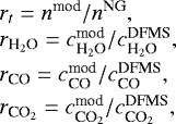 (5)
(5)
where nmod and nNG are the overall gas densities at the position of the orbiter computed and measured by the nude gauge of COPS,  ,
,  ,
,  are the relative abundances of H2O, CO, and CO2 from the simulation, and
  ,
,  ,
,  are the relative abundances measured by DFMS.
Since the flux along a flowline is F = nv (where n and v are local gas density and velocity) and taking into account that v tends to const. with increasing nucleocentric distance, the flux at the positions of the orbiter is F ∝ n. Therefore, the mean ratio nmod∕nNG shows if the flux from the element was in general under- or overestimated. The current (at iteration i) flux from the surface element is
 (6)
(6)
The new (i.e. for the next iteration) inhomogeneity factors  ,
, ,
, for each surface cell are computed from the equations
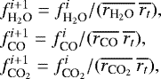 (7)
(7)
where i is the index of iteration and the bar in  means averaging over flowlines originated from a given surface cell. As variations in the flux affect the flow in general it is necessary torepeat iteratively simulations for the whole rotational period with the new flux distribution.
Since observational data are limited, some of the surface elements may have no data (i.e. are empty cells). Therefore, it is necessary toexpand the data from non-empty cells in order to cover the whole surface. This procedure consists in consecutive iterations in which, in the loop over empty cells, we assign for the cell the averaged data from the neighbouring non-empty cells. The iterations are repeated until all cells contain data. An example of this process is illustrated in Fig. 6.
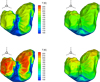 |
Fig. 4 Distribution of surface temperature of water ice (top panels) and of non-icy surface (bottom panels) for two types of models: instantaneous energy input (left panels) and rotation-averaged energy input (right panels). Computations made for Oct. 1, 2014, 07:08:00 UTC, the Sun being nearly in the plane Y = 0 and at 40° from +X. |
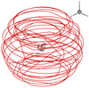 |
Fig. 5 Trajectory of Rosetta during 1–15 October 2014 (in the nucleus attached frame). |
4 Results
For most ofour computations we used our coma grid with the resolution 2.5° × 2.5°, which gives 7776 surface cells.
We have fitted the data acquired in August–November 2014 by the ROSINA instrument (pressure gauge COPS and DFMS), which are described in detail in Le Roy et al. (2015). In the course of this period, the heliocentric distance changed from 3.62 to 2.87 AU. In order to take into account accurately the variation of gas production, we divided this period into ten-day segments, which corresponds to ~ 2% variation of rh. For each time segment, we performed simulations of the gas outflow (with corresponding rh) for one rotational period split into 72 instants (i.e. 10-min intervals).
During the period August–November 2014, the COPS made about 125 000 measurements (cleaned from the firing events) and the DFMS made about 6000 measurements. For adjustment we used time instances corresponding to the COPS measurements and the DFMS data were linearly interpolated (this implies that the composition of the gas mixture does not vary significantly on shorter timescales). In one time segment, we had typically about 10 000 measurements. Since for a grid with resolution 2.5° × 2.5° the number of surface elements is 7776, for one 10-day time segment the number of samples per surface element is very poor and a large part of the surface may not be covered at all. To improve the statistics, we usually combined several successivetime segments. This implicitly assumes that inhomogeneity factors do not depend on the variation of rh.
We started from the assumption of a homogeneous surface (i.e. inhomogeneity factors were the same all over the surface) with two types of energy input: instantaneous (w = 0) and completely rotation-averaged (w = 1). The H2O production was assumed to be set by an icy fraction  , and the total CO and CO2 production rates were, respectively, 2.0 × 1025 and 3.0 × 1024 molec s−1 (with fCO = 1 and
  = 1).
= 1).
Figure A.1 shows the comparison of the simulated gas density and velocity distribution. In the case in which w = 1, owing to the more uniform income energy distribution over the surface, the bottom of the “neck” region is relatively more active and the flow field is more symmetric with respect to the axis of rotation Z. Figure A.2 shows a comparison of the gas density in the position of the Rosetta orbiter predicted by models and COPS measurements for the period August–November 2014, with zoom on the period October 8–12. The model with averaged energy input shows less amplitude of density variation during the rotation period and it corresponds better to the measured data when the orbiter passes above the southern hemisphere (sub-spacecraft latitude, Z < 0).
To numerically quantify the agreement between the model and the observations, we computed the mean (δx) and the dispersion (σx) of relative difference ( ) in the simulated and measured data x:
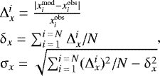 (8)
(8)
where N is a number of points in the segment of comparison, and  ,
,  are comparable parameters (n,
  ,
,  , cCO) in our simulations and in the measurements. The results for the models with homogeneous nucleus when w = 0 and w = 1 are given in Table 1 (cases f033c1w00 and f033c1w10, respectively). According to these criteria, the model with w = 1 practically fits the measured densities two times better than the model in which w = 0.
Figure A.3 shows an example of the sample volume distribution for surface elements for the period August–November 2014. As expected in the southern (Z < 0) hemisphere, statistics are very poor. In the northern (Z > 0) hemisphere, the number of samples per surface element reaches 100.
The distribution of the  , fCO, and
  after two iterations of adaptation (with gas outflow simulation based on Euler equations) is shown in Fig. A.4. The EE method was used for the initial iterations of adjustment due to its high computational efficiency and acceptable validity in the prediction of the spatial gas density distribution (see Lukyanov et al. 2005; Crifo et al. 2016). Figure A.5 shows a comparison of the measured and simulated gas densities (after adaptation of the surface inhomogeneity factors). The mean and dispersion of relative difference in simulated and measured gas densities are given in Table 1 (cases f002a1w00 and f002a1w10). After adaptation of the surface inhomogeneity factors, the model in which w = 0 improves the agreement with observations on gas density nearly twofold. The model in which w = 1 produced the same agreement in the overall density but very much improved agreement for the relative abundance of CO.
For further adjustment, we used only the model in which w = 0 and for the gas outflow simulations we applied the DSMC method. For the last iterations we used the DSMC method, which is less computationally efficient than the EE but more physically adequate. In order to reduce computational expenses, for the adjustment we restricted the period of study to September 15–October 30, 2014. The distribution of the  , fCO, and
  after two additional iterations of adaptation is shown in Fig. A.6. Additionally, for this distribution of inhomogeneity factors, the gas outflow was computed by the EE method as well. Figure A.7 shows the distributions of gas density and velocity simulated by the EE and the DSMC methods. The results of the density simulation by gas-dynamic and gas-kinetic codes are in a reasonable agreement but the velocity distribution near the nucleus differs noticeably.
Figure A.8 shows a comparison of the gas density in the position of the Rosetta orbiter predicted by models based on the Euler equations and the DSMC approach with instantaneous energy input and COPS measurements for the period September 15–October 30 and the period October 8–12 after adaptation of the surface inhomogeneity factors. The mean and dispersion of the relative difference in simulated and measured gas density are given in Table 1 (cases f004a3w00 for the EE method and m004a3w00 for the DSMC). From these criteria, it follows that for the used inhomogeneity pattern, both methods (EE and DSMC) are almost equally close to the measured density but the DSMC gives better agreement with relative abundances. The density variation predicted by the EE method has more sharp gradients than the DSMC. In both predictions there is an extra or split peak at about 3 h on October 10.
Figure A.9 shows a comparison of the relative abundances of H2O, CO, and CO2 in the position of the Rosetta orbiter predicted by the DSMC model after four iterations of the surface inhomogeneity factors adjustment for the period from September 15, 2014 to October 30, 2014 and during October 8–12, 2014. In the period September 15–October 30, the model initially underestimates the relative abundance of CO but then overestimates it at the approach to the end of the time segment. This is a consequence of the constant total production rate of CO postulated in the model.
Figure A.10 shows the variation of total gas production during one rotation period at rh = 3.21 AU. Dashed lines show gas production for the homogeneous nucleus, solid lines show gas production after adjustment of the surface inhomogeneity factors. We stop the adjustment procedure after four iterations when the mean relative difference between simulated and measured parameters is about 30%. This was caused by the following reasons: (1) each iteration of the adjustment procedure needs a considerable amount of computations (13 time segments × 72 time instants); (2) since we started our work, the shape model used in our simulations has improved (especially in the southern hemisphere) and this may affect the gas distribution; (3) the measurements have error bars of the order of 10–20%. Therefore, we decided that further adjustment is not worth the effort.
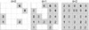 |
Fig. 6 Example of flooding algorithm. Initial distribution of data (left panel), first iteration (middle panel), and the last iteration (right panel). |
Comparison of the model predictions with COPS and DFMS measurements in different time segments.
5 Conclusion
In the case of nuclei with homogeneous surface (i.e. inhomogeneity factors are the same all over the surface), the model with energy input averaged over period of rotation (w = 1) better fits the ROSINA data than the model with instantaneous energy input (w = 0): the mean relative difference in total gas density is about 50% versus about 100%. The amplitude of density variation is less in the model in which w = 1 since it depends only on the instrument location in the coma (the gas production remains practically constant during the rotation). As follows from a distribution of the surface temperature (Fig. 4), in the model in which w = 1 more active surface (due to a higher temperature) concentrates on top of the shape, as the part which is exposed for the longest time (this behaviour is consistent with the results of a further adjustment of surface inhomogeneity factors). However, the adjustment of surface inhomogeneity in the case of w = 1 does not improve the agreement with measured data and this means that gas production should be essentially dependent on instantaneous illumination conditions.
Adaptation of surface inhomogeneity strongly improves the fit of the model in which w = 0. Final (after four iterations of adaptation) distribution of the surface inhomogeneity factors shows that for all components (H2O, CO, and CO2) the most productive surface is located around the northern (Z > 0) peaks and crests of the shape. We emphasize the difference between “more active” and “more productive” surfaces. The more active surface has a greater production rate per square metre in comparison with other surfaces (possibly having other surface properties or/and having other illumination conditions). The more productive surface has greater production rate per square metre in comparison with other surface at the same illumination conditions.
The final distribution of the surface inhomogeneity (Fig. A.6) is quite different from the results presented in Fougere et al. (2016a,b) and Marschall et al. (2016). These studies came to the conclusion that the most productive surface is located in the neck region of the shape. According to our results, the neck is also relatively highly productive (only for H2O) but the most productive areas (for all species) are located around the northern (Z > 0) peaks and crests of the shape. The reason for this discrepancy could be that the flow from the bottom of the neck region and the flow formed by the interaction of fluxes from the lobes (see Fig. A.7) may result in a similar density in the points of measurements, that is, it is possible to fit the ROSINA data by several models of gas production. This naturally brings us to the necessity of fitting to the observational data from other Rosetta instruments as well (and this work is currently in progress).
The results of our analysis show that in the considered time span the outgassing is defined mostly by instantaneous illumination conditions (which are strongly dependent on the nucleus shape) and local properties (inhomogeneity) of the surface. At the same time, owing to the rather rarefied conditions of gas outflow (and therefore fast dissipation of flow structures), small-scale topographical features do not affect the flow noticeably for the present in situ observations (made at altitudes of 10–100 km). In the considered conditions, “small-scale” means comparable with the mean free path of the molecules near the surface, that is, on the order of 100 m. However, due to the lack of information about the near-nucleus gas coma of other comets, it is not without problems to generalize these results to all comets.
As an interesting practical observation, it was found that the results of simulations based on the fluid approach (Euler equations) and by the DSMC give close fits to observational data on total density but less good fits on composition. This proves that the fluid approach (much more computationally effective) could be applied for approximate simulations of the coma in spite of strong rarefaction of the flow.
Acknowledgements
We thank the French CNES centre (and personally Philippe Gaudon) for uninterrupted support during the whole Rosetta project. Rosetta is an ESA mission with contributions from its member states and NASA. We acknowledge herewith the work of the whole ESA Rosetta team. Work on ROSINA at the University of Bern was funded by the State of Bern, the Swiss National Science Foundation, and by the European Space Agency PRODEX programme.
Appendix A Additional figures
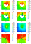 |
Fig. A.1 Example of distribution of gas density (first and third rows) and velocity (second and bottom rows) in the model with instantaneous (left panels) and rotation-averaged (right panels) energy input for a homogeneous nucleus. The flow streamlines are shown in black in the panels with the distribution of gas velocity. Computations were made for rh = 3.266 (October 1, 2014). The Sun is in the Y = 0 plane at 41° from the +X axis in an anticlockwise direction. |
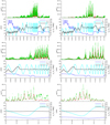 |
Fig. A.2 Comparison of gas density at position of Rosetta orbiter predicted by models (nmod, green) with homogeneous surface (left panels: instantaneous energy input, right panels: rotation-averaged energy input) and COPS measurements (nNG, red): in August–November 2014 (top row), in September 15–October 30, 2014 (middle row), and in October 8–12 (bottom row). The bottom part of each panel shows cometocentric distance Δ, colatitude θSC, and phase angle α of the orbiter. The horizontal axis shows the date (yy-mm-dd). |
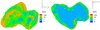 |
Fig. A.3 Statistics on streamlines per surface element for the case of instantaneous energy input for the period August–November 2014. |
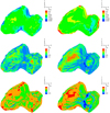 |
Fig. A.4 Distribution of surface inhomogeneity factors |


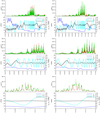 |
Fig. A.5 Comparison of gas density at the position of the Rosetta orbiter predicted by models (green) with inhomogeneous (after two iterations) nucleus (left panels: instantaneous, right panels: rotation-averaged energy input) and COPS measurements (red): in August–November 2014 (top row), in September 15–October 30, 2014 (middle row), and in October 8–12 (bottom row). The bottom part of each panel shows cometocentric distance Δ, colatitude θSC, and phase angle α of the orbiter. The horizontal axis shows the date (yy-mm-dd). |
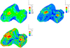 |
Fig. A.6 Distribution of surface inhomogeneity factors |


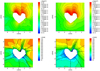 |
Fig. A.7 Distribution of gas density (top panels) and velocity (bottom panels) from EE (left panels) and DSMC (right panels) after adjustment. The flow streamlines are shown in black in the panels with the distribution of gas velocity. Computations were made for rh = 3.21 (October 10,2014). The Sun is in the Y = 0 plane at 40° from the +X axis in an anticlockwise direction. |
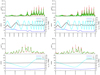 |
Fig. A.8 Comparison of gas density at the position of the Rosetta orbiter predicted by models with inhomogeneous (after four iterations) nucleus (green) and COPS measurements (red): in September 15–October 30, 2014 (top row), in October 8–12 (bottom row). Left panels: DSMC, right panels: EE. The bottom part of each panel shows cometocentric distance Δ, colatitude θSC, and phase angle α of the orbiter. The horizontal axis shows the date (yy-mm-dd). |
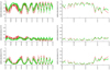 |
Fig. A.9 Comparison of relative abundances of H2O (top panels), CO (middle panels), and CO2 (bottom panels) at the position of the Rosetta orbiter predicted by the DSMC solution (green) with inhomogeneous (after four iterations) nucleus and COPS measurements (red): in September 15–October 30, 2014 (left panels), in October 8–12 (right panels). |
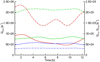 |
Fig. A.10 Variation of total gas production during one rotation period (at rh = 3.21 AU): red lines |


References
- Balsiger, H., Altwegg, K., Bochsler, P., et al. 2007, Space Sci. Rev., 128, 745 [NASA ADS] [CrossRef] [Google Scholar]
- Bieler, A., Altwegg, K., Balsiger, H., et al. 2015, A&A, 583, A7 [NASA ADS] [CrossRef] [EDP Sciences] [Google Scholar]
- Bird, G. 1994, Molecular Gas Dynamics and the Direct Simulation of Gas Flows, v. 1 (Oxford, UK: Clarendon Press) [Google Scholar]
- Cercignani, C. 1981, in Progress in Astronautics and Aeronautics (New York, NY: American Institute of Aeronautics and Astronautics) 74, 305 [NASA ADS] [Google Scholar]
- Crifo, J.-F., Zakharov, V. V., Rodionov, A. V., & Lukyanov, G. A. 2016, in AIP Conf. Ser., 1786, 160007 [Google Scholar]
- Fougere, N., Altwegg, K., Berthelier, J.-J., et al. 2016a, A&A, 588, A134 [NASA ADS] [CrossRef] [EDP Sciences] [Google Scholar]
- Fougere, N., Altwegg, K., Berthelier, J.-J., et al. 2016b, MNRAS, 462, S156 [CrossRef] [Google Scholar]
- Jurado, E., Martin, T., Canalias, E., et al. 2016, Acta Astron., 125, 65 [CrossRef] [Google Scholar]
- Kramer, T., Läuter, M., Rubin, M., & Altwegg, K. 2017, MNRAS, 469, S20 [CrossRef] [Google Scholar]
- Le Roy, L., Altwegg, K., Balsiger, H., et al. 2015, A&A, 583, A1 [NASA ADS] [CrossRef] [EDP Sciences] [Google Scholar]
- Lukyanov, G. A., Zakharov, V. V., Rodionov, A. V., & Crifo, J.-F. 2005, in AIP Conf. Ser., 762, 331 [NASA ADS] [CrossRef] [Google Scholar]
- Marschall, R., Su, C. C., Liao, Y., et al. 2016, A&A, 589, A90 [NASA ADS] [CrossRef] [EDP Sciences] [Google Scholar]
- Rodionov, A. V., & Crifo, J.-F. 2006, Adv. Space Res., 38, 1923 [NASA ADS] [CrossRef] [Google Scholar]
- Rodionov, A. V., Crifo, J.-F., Szegö, K., Lagerros, J., & Fulle, M. 2002, Planet. Space Sci., 50, 983 [NASA ADS] [CrossRef] [Google Scholar]
- Szegö, K., Crifo, J.-F., Rodionov, A. V., & Fulle, M. 2002, Earth Moon Planets, 90, 435 [NASA ADS] [CrossRef] [Google Scholar]
All Tables
Comparison of the model predictions with COPS and DFMS measurements in different time segments.
All Figures
|
Fig. 1 Shape models: RMOC shape 3 (first row) and effective surface model with resolution 1o × 1o (second row), 2.5o × 2.5o (third row), 5o × 5o (bottom row). Left column: view (from −Y) on the full shape. Right column: scaled-up part from the red box (with a surface grid shown in black). |
| In the text | |
|
Fig. 2 Example of the computational grid: near the surface (left panel) and close to the outer boundary (right panel). The blocs comprising the “football” grid are shown in different color. |
| In the text | |
|
Fig. 3 Input energy distribution in the case of instantaneous energy input (left panel) and rotation averaged energy input (right panel). Computations made for Oct. 1, 2014, 07:08:00 UTC, the Sun being nearly in the plane Y = 0 and at 40° from +X. |
| In the text | |
|
Fig. 4 Distribution of surface temperature of water ice (top panels) and of non-icy surface (bottom panels) for two types of models: instantaneous energy input (left panels) and rotation-averaged energy input (right panels). Computations made for Oct. 1, 2014, 07:08:00 UTC, the Sun being nearly in the plane Y = 0 and at 40° from +X. |
| In the text | |
|
Fig. 5 Trajectory of Rosetta during 1–15 October 2014 (in the nucleus attached frame). |
| In the text | |
|
Fig. 6 Example of flooding algorithm. Initial distribution of data (left panel), first iteration (middle panel), and the last iteration (right panel). |
| In the text | |
|
Fig. A.1 Example of distribution of gas density (first and third rows) and velocity (second and bottom rows) in the model with instantaneous (left panels) and rotation-averaged (right panels) energy input for a homogeneous nucleus. The flow streamlines are shown in black in the panels with the distribution of gas velocity. Computations were made for rh = 3.266 (October 1, 2014). The Sun is in the Y = 0 plane at 41° from the +X axis in an anticlockwise direction. |
| In the text | |
|
Fig. A.2 Comparison of gas density at position of Rosetta orbiter predicted by models (nmod, green) with homogeneous surface (left panels: instantaneous energy input, right panels: rotation-averaged energy input) and COPS measurements (nNG, red): in August–November 2014 (top row), in September 15–October 30, 2014 (middle row), and in October 8–12 (bottom row). The bottom part of each panel shows cometocentric distance Δ, colatitude θSC, and phase angle α of the orbiter. The horizontal axis shows the date (yy-mm-dd). |
| In the text | |
|
Fig. A.3 Statistics on streamlines per surface element for the case of instantaneous energy input for the period August–November 2014. |
| In the text | |
|
Fig. A.4 Distribution of surface inhomogeneity factors |
| In the text | |
|
Fig. A.5 Comparison of gas density at the position of the Rosetta orbiter predicted by models (green) with inhomogeneous (after two iterations) nucleus (left panels: instantaneous, right panels: rotation-averaged energy input) and COPS measurements (red): in August–November 2014 (top row), in September 15–October 30, 2014 (middle row), and in October 8–12 (bottom row). The bottom part of each panel shows cometocentric distance Δ, colatitude θSC, and phase angle α of the orbiter. The horizontal axis shows the date (yy-mm-dd). |
| In the text | |
|
Fig. A.6 Distribution of surface inhomogeneity factors |
| In the text | |
|
Fig. A.7 Distribution of gas density (top panels) and velocity (bottom panels) from EE (left panels) and DSMC (right panels) after adjustment. The flow streamlines are shown in black in the panels with the distribution of gas velocity. Computations were made for rh = 3.21 (October 10,2014). The Sun is in the Y = 0 plane at 40° from the +X axis in an anticlockwise direction. |
| In the text | |
|
Fig. A.8 Comparison of gas density at the position of the Rosetta orbiter predicted by models with inhomogeneous (after four iterations) nucleus (green) and COPS measurements (red): in September 15–October 30, 2014 (top row), in October 8–12 (bottom row). Left panels: DSMC, right panels: EE. The bottom part of each panel shows cometocentric distance Δ, colatitude θSC, and phase angle α of the orbiter. The horizontal axis shows the date (yy-mm-dd). |
| In the text | |
|
Fig. A.9 Comparison of relative abundances of H2O (top panels), CO (middle panels), and CO2 (bottom panels) at the position of the Rosetta orbiter predicted by the DSMC solution (green) with inhomogeneous (after four iterations) nucleus and COPS measurements (red): in September 15–October 30, 2014 (left panels), in October 8–12 (right panels). |
| In the text | |
|
Fig. A.10 Variation of total gas production during one rotation period (at rh = 3.21 AU): red lines |
| In the text | |
Current usage metrics show cumulative count of Article Views (full-text article views including HTML views, PDF and ePub downloads, according to the available data) and Abstracts Views on Vision4Press platform.
Data correspond to usage on the plateform after 2015. The current usage metrics is available 48-96 hours after online publication and is updated daily on week days.
Initial download of the metrics may take a while.