| Issue |
A&A
Volume 618, October 2018
|
|
|---|---|---|
| Article Number | A127 | |
| Number of page(s) | 5 | |
| Section | Extragalactic astronomy | |
| DOI | https://doi.org/10.1051/0004-6361/201832655 | |
| Published online | 18 October 2018 | |
AGN mass estimates in large spectroscopic surveys: the effect of host galaxy light
1
Università degli Studi di Milano–Bicocca, Dipartimento di Fisica “G. Occhialini”,
Piazza della Scienza 3,
20126
Milano,
Italy
e-mail: l.varisco4@campus.unimib.it
2
INAF – Osservatorio Astronomico di Trieste,
via Tiepolo 11,
34131
Trieste,
Italy
3
INFN, Sezione di Milano–Bicocca,
Piazza della Scienza 3,
20126
Milano,
Italy
Received:
17
January
2018
Accepted:
16
March
2018
Virial–based methods for estimating active supermassive black hole masses are now commonly used on extremely large spectroscopic quasar catalogs. Most spectral analyses, though, do not pay enough attention to the detailed continuum decomposition. To understand how this affects virial mass estimates, we test the influence of host galaxy light on them, along with a Balmer continuum component. A detailed fit with the new spectroscopic analysis software QSFIT demonstrates that the presence or absence of continuum components does not significantly affect the virial-based results for our sample. Taking a host galaxy component into consideration or not, instead, affects the emission line fitting in a more pronounced way at lower redshifts, where in fact we observe dimmer quasars and more visible host galaxies.
Key words: galaxies: active / quasars: supermassive black holes / black hole physics / quasars: general
© ESO 2018
1 Introduction
Massive black holes (MBHs), commonly observed in the centers of massive galaxies, can be fully characterized by only two parameters: their masses and their spins (see e.g., Sesana et al. 2014, and references therein). Since MBH spins affect the dynamics of matter only within their innermost few gravitational radii, spins are usually constrained through observationally challenging X-ray spectroscopy complemented with relativistic modeling of broad iron lines (see Brenneman 2013; Reynolds 2014, for recent reviews on the topic1). On the other hand, MBH masses can dominate the dynamics of gas and stars up to parsec scales (depending on the MBH masses and the host properties; see e.g., Dotti et al. 2012) and are therefore easier to constrain. Direct measurements are possible in a limited number of cases, through orbital fitting of single stars as for the case of our Galaxy (see e.g., Gillessen et al. 2009a,b; Genzel et al. 2010; Meyer et al. 2012), through fitting the dynamics of megamaser emitting disks (Braatz et al. 1997; Greene et al. 2010; Van Den Bosch et al. 2016), or by modeling the dynamics of whole stellar and/or gaseous populations in the immediate vicinities of the MBHs (e.g., Gebhardt et al. 2003; Ferrarese & Ford 2005; Van Der Marel et al. 1998, for a review).
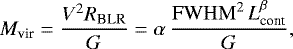
Alternative options for estimating MBH masses are available for the subclass of Type I active MBHs (AGN). A widely used method to perform MBH mass estimates for this class of sources is based on the virial theorem (see Peterson 2014, and references therein). The main assumption in this approach is that the gas in the sub-parsec region emitting the broad lines (BLR) is virialized and its dynamic is dominated by the central MBH. Therefore the virial MBH mass is determined by:
 (1)
(1)
where V is the virial velocity and R the size of the BLR. Assuming that broad emission lines (BELs) are Doppler broadened due to the virial motion of the BLR, the full width at half maximum (FWHM) of the BELs can be used as a proxy of the emitting gas velocities. Moreover, through an analysis of the time-delayed response of BELs to variations of the continuum, reverberation mapping campaigns provided estimates of the BLR size. Reverberation mapping studies have also revealed the so – called size – luminosity relation between the monochromatic luminosity of the AGN continuum and the BLR size (Kaspi et al. 2000; Bentz et al. 2006). Continuum luminosity can therefore be used as a proxy of the BLR size. Hence, MBH mass can be estimated by means of a fudge factor α that includes uncertainties on BLR shape and dynamics (see e.g., Decarli 2011). α factor can however be constrained self-consistently via reverberation mapping studies in cases where extremely high-quality and high-coverage data are available (Brewer et al. 2011; Pancoast et al. 2012).
Shen et al. (2011) presented a systematic study of the SDSS DR7 Quasar Catalogue (Schneider et al. 2010), in which every spectrum is automatically fitted with a power-law continuum, along with broad and narrow emission lines and an iron template. MBH masses were constrained from the FWHM of different BELs (depending on the AGN redshift), and the monochromatic luminosity in the proximity of the BEL used. In this paper we re-examine all the AGN in the SDSS-DR10 catalog by performing an independent fit of each AGN spectrum with the publicly available QSFIT code (Calderone et al. 2017)2. In addition to the spectral features related to the accreting MBH, the code includes an elliptical galactic template (Polletta et al. 2007). This feature is important for two reasons: (i) it could contribute to the monochromatic luminosity, resulting in the overestimation of single epoch MBH masses, and (ii) depending on its intensity and spectral shape, it could affect the BEL shape hence, the FWHM. The contamination from the host galaxy can be drastically reduced in multiple ways, for example, by taking high-angular-resolution nuclear spectra, or by considering only the varying component of the emission from multi-epoch spectral studies of the same AGN (as done in reverberation mapping). We stress however that none of these approaches can be applied to very large AGN samples characterized by broad distributions of AGN luminosities and redshifts, such as the SDSS catalog. Therefore, in order to maximize the payoff of such large surveys, the fitting of the host component is mandatory. Some methods have been proposed in the literature to estimate the contamination due to the host galaxy in continuum luminosity measurements. Shen et al. (2011) compute a statistical analysis on low-redshift sources (in which we expect a higher host-galaxy contamination) and provide an empirical fitting formula. In their work the resulting host galaxy contamination is on average ~ 15% of the the continuum luminosity at 5100 Å on low-redshift sources (z ≲ 0.5). Other authors proposed different approaches such as the use of the equivalent width of the line Ca II K line at 3934 Åas a proxy of the degree of host contamination (Greene & Ho 2005).
Different single epoch relations have been proposed to remove the host galaxy contamination (e.g., Eqs. (6) and (7) of Greene & Ho 2005; Bongiorno et al. 2014), based on empirical relations observed on large samples of AGNs. Hence these relations are only able to estimate host galaxy contributions on average, not on individual sources. In this work, we analyzed each source individually to isolate the host galaxy contribution and avoid any possible bias introduced by the choice of the sample for the empirical relations.
The paper is organized as follows: in Sect. 2 we discuss how we select the AGN sample used and review the main features of the spectral fitting implemented in QSFIT. In Sect. 3 we discuss our results and how they depend on the redshift and on the AGN properties. Finally, in Sect. 4 we draw our conclusions and discuss possible future improvements.
2 Sample selection and data analysis
Our prime sample was composed of the 10578 sources in the QSFIT catalog (version 1.2 Calderone et al. 2017) with z< 0.8 for which a measurement of the AGN continuum luminosity at 5100 Åand of the FWHMHβ was available in Shen’s catalog (Shen et al. 2011). We analyzed the SDSS-DR10 optical spectra using the QSFIT software (version 1.2 Calderone et al. 2017). Each spectrum is de-reddened following the prescription by Cardelli et al. (1989) and O’Donnell (1994), then transformed to rest frame and finally analyzed using the QSFIT recipe which simultaneously fits all the spectral components visible in the observed wavelength range. QSFIT uses a power law to model the AGN broad band, a component to account for the Balmer continuum (following the recipe by Grandi 1982; Dietrich et al. 2002), the Polletta et al. (2007) elliptical galaxy template to account for the host galaxy emission, the iron templates by Vestergaard & Wilkes (2001) and Véron-Cetty et al. (2005) at UV and optical wavelengths respectively, and several Gaussian profiles to account for the most commonly observed emission lines. We collected all the output values and extracted the relevant quantities for the purpose of this work, namely the λLλ continuum luminosity at 5100 Å (L5100), the Balmer continuum contribution, and the FWHM of the Hβ emission line.
The inclusion of the Balmer continuum component in the fit procedure affects the slope of the continuum and could, as a consequence, modify the continuum at longer wavelengths. By running the analysis with and without considering the Balmer continuum component (by setting the !QSFIT_OPT.balmer option to 0) we quantify its impact on the MBH mass estimates.
We selected the sources for which the fit quality flag of the continuum at 5100 Åand of the Hβ broad emission line components were good (namely CONT5100_QUALITY and br_Hb_QUALITY simultaneously equal to 0) for both standard and without Balmer component analysis. The final sample consisted of 9107 sources.
In the following, results of the standard analysis will be flagged as  and FWHM
 , while the quantities obtained by disabling the Balmer continuum component will be flagged as
  and FWHM
 .
.
3 Supermassive black hole mass estimates
Figure 1 shows the results of our full spectral fitting procedure (including the Balmer continuum component; see the discussion above) performed over two AGN-host galaxy systems, exemplifying the different possible degrees of host galaxy contribution to SDSS spectra. The upper panel shows the SDSS image and spectrum of SDSS J032545.70–000820.6, a source with a host galaxy significantly fainter than the AGN, while the lower panel shows SDSS J155053.16+052112.1, an AGN hosted in a brighter galaxy. Other than being clearly different in the SDSS images (host galaxy emission almost unresolved in the upper panel), the two nuclei significantly differ in their spectra. The spectrum of SDSS J032545.70–000820.6 is well fitted without any need for a relevant host galaxy contribution. On the other hand, the analysis performed on the spectrum of SDSS J155053.16+052112.1 reveals a dominant contribution of the host galaxy light in the continuum emission. In this case an analysis performed without considering the host galaxy contribution would lead to an overestimate of at least a factor 1.3 in the 5100 Å continuum3. A poor estimate of the continuum could also affect the emission line profile reconstruction: S11 fits BELs with a combination of up to four Gaussian profiles in order to account for asymmetries, while in 82% of cases we require only one component to achieve a good fit4.
After running the two variants of spectral fitting discussed in Sect. 2 over our entire sample, we proceed to estimating the MBH masses (M) using the two following calibrations:
 (2)
(2)
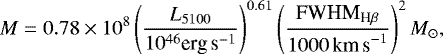
originally proposed by McLure & Dunlop (2004), and
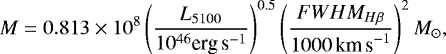 (3)
(3)
proposed by Vestergaard & Peterson (2006). Neither calibration includes the host galaxy contribution. These relations have been chosen to compare our findings with the estimates presented in S11 in order to quantify the effect of the host galaxy light on the estimate of M. The masses obtained from the full fitting procedure (i.e., the masses obtained using  and FWHM
 in Eqs. (2) and (3)) are dubbed
  , while with
  we indicate the mass estimates from the fitting that does not include the Balmer contribution.
Figure 2 presents an overview of the results of our fitting procedures. In the upper left panel we show a comparison between the distribution of 5100 Å continuum luminosity measured by S11 ( ) and the distributions of
  and
and  obtained with the QSFIT analysis. While the parameters obtained with and without the Balmer component are consistent (see also the other panels in Fig. 2 and the following discussion), the
  distribution clearly differs from the others, in that it is completely missing the low-luminosity tail: the less luminous AGNs have more likely a relevant host galaxy component, that contributes significantly to the 5100 Å monochromatic luminosity.
The same comparison between the FWHMHβ distributions is shown in the lower left panel. Again, the FWHM distributions obtained with or without including the Balmer component in the QSFIT analysis are comparable, while S11 estimate systematically narrower FWHM. Given that the QSFIT results obtained with or without Balmer continuum component are substantially consistent, the resulting distribution of  and
and  is compatible, as shown in the right panel of Fig. 2. As a consequence, in the following we limit our comparison to the masses presented in S11 and those obtained through the full QSFIT analysis (
 ).
).
Figure 3 shows the main result of our investigation. The two-dimensional (2D) color-coded histogram indicates the redshift distribution of the MS11 to  ratio. The different slope of the continuum luminosity at 5100 Åand the different normalization in the two calibrations affect the ratio MS11∕M distributions shown with two-dimensional histograms in Fig. 3. Indeed in Eq. (2) the L5100 slope is 0.61 resulting in a MS11∕M ratio generally ≳1 for McLure & Dunlop (2004) calibration; while in Eq. (3) the L5100 slope is 0.5 resulting in a MS11∕M distribution ≲ 1 for Vestergaard & Peterson (2006) calibration. The two masses are comparable within a factor of approximately three at all redshifts, but a large scatter is present, mostly due to the different FWHMHβ estimates that enter quadratically in Eqs. (2) and (3). This indicates how much the single epoch virial estimates are affected by the inclusion (or not) of a host galaxy component and by the decision on the number of Gaussian profiles used to fit the BELs. As a second-order correction, on average, S11 estimates a higher mass compared to QSFIT at low redshift, as highlighted by the asymmetric distribution of the sources in Fig. 3. To investigate how a correct decomposition of the observed continuum affects the virial mass estimates, we consider a “mixed” virial supermassive black hole mass estimate Mmix, calculated using S11 FWHM and our AGN continuum luminosity. The comparison between MS11 and Mmix is also shown in Fig. 3 using density contours. Using the same value for the FWHMHβ drastically reduces the scattering, while the redshift dependence of the host galaxy contamination is emphasized: At lower redshifts, where the host galaxy contribution is likely more relevant, the S11 result overestimates the virial mass calculated in this work. At high redshifts, instead, the two mass estimates are comparable; quasars are likely brighter and the host galaxy contribution is much more diluted in the continuum emission.
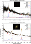 |
Fig. 1 SDSS spectra and images of SDSS J032545.70−000820.6 (z ≃ 0.7; upper panel)and SDSS J155053.16+052112.1 (z ≃ 0.1; lower panel). In each spectrum, SDSS data with respective errors (black lines) are compared with the QSFIT model (orange solid line). The red dashed line is the continuum component, while the red solid line includes both AGN and host galaxy continuum. The dot-dashed green line is the Balmer continuum component; the green solid line is the iron template. Broad emission lines are shown with solid blue lines, while narrow emission lines with solid brown lines. The solid purple line is the sum of all the “unknown” lines. The spatial region from which the SDSS spectra were obtained is shown in the SDSS images with a green circle with a diameter of 3 arcsec. The two sources have significantly different contributions from the host galaxy: this is evident both in the SDSS images and in the spectra. In our fitting procedure we did not fix the FWHM and fluxes ratio of the [OIII] doublet. This affects individual features of the [OIII] doublet, but does not affect the mass estimates. |
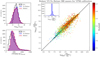 |
Fig. 2 Left panels: distributions of 5100 Å continuum luminosity (upper) and FWHMHβ (lower). Black histograms show results from S11. Red and blue filled histograms are the QSFIT results obtained including and without the Balmer continuum component, respectively. Right panel: comparison between |


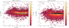 |
Fig. 3 Ratio of virial masses of S11 and this work as a function of redshift. The color-coded two-dimensional histogram refers to ratios in which the MBH virial masses |

4 Conclusions
We present the results of an automated spectral analysis of a subsample of the SDSS DR10 quasar catalog. Our analysis, performed using the public code QSFIT, fits the SDSS spectra including a host galaxy template together with the AGN components (power-law continuum, broad and narrow emission lines, and a Balmer). We used the broad FWHMHβ and the monochromatic luminosity at 5100 Å to estimate the MBH masses responsible for the nuclear emission.
We demonstrated that the inclusion of the Balmer does not significantly affect the Hβ mass estimates in our sample, while the inclusion of a host galaxy component can significantly change both the BEL shape and the 5100 ÅAGN monochromatic luminosity. In order to quantify such an effect, we compared our estimates with those presented by S11. We find a general agreement with S11, with the MBH mass estimates being consistent within a factor of three. The main cause of the observed scattering is due to the quadratic dependence of M on the FWHMHβ, the latter being dependent on the continuum assumed and on the number of Gaussian profiles allowed in the fit. Considering the intrinsic uncertainties associated with the single epoch estimators, which are of the order of approximately four, our estimates are consistent with those of S11.
Once the effect of the different FWHM of the broad Hβ is removed (using the same values measured by S11), the effect of including a host galaxy template becomes evident. Depending on the calibrations used, S11 either overestimates M by about a factor of 2, or, when the calibration from Vestergaard & Peterson (2006) is assumed (Eq. (3)), a significantly better agreement is reached, with the masses becoming compatible within a factor of 1.5. In this last case, at low redshift, where the host galaxy significantly contributes to the continuum luminosity, our mass estimates are still slightly lower than those of S11. At higher redshift (z ≳ 0.6), the estimates instead converge within 0.15 dex, the AGN overwhelming any contribution from the host galaxy.
References
- Bentz, M. C., Peterson, B. M., Pogge, R. W., et al. 2006, ApJ, 644, 133 [NASA ADS] [CrossRef] [Google Scholar]
- Bongiorno, A., Maiolino, R., Brusa, M., et al. 2014, MNRAS, 443, 2077 [NASA ADS] [CrossRef] [Google Scholar]
- Braatz, J. A., Wilson, A. S., & Henkel, C. 1997, ApJS, 110, 321 [NASA ADS] [CrossRef] [Google Scholar]
- Brewer, B. J., Lewis, G. F., Belokurov, V., et al. 2011, ApJ, 733, L33 [NASA ADS] [CrossRef] [Google Scholar]
- Brenneman, L. 2013, Measuring the Angular Momentum of Supermassive Black Holes, (New York: Springer) [CrossRef] [Google Scholar]
- Calderone, G., Nicastro, L., Ghisellini, G., et al. 2017, MNRAS, 432, 4051 [NASA ADS] [CrossRef] [Google Scholar]
- Campitiello, S., Ghisellini, G., Sbarrato, T., & Calderone, G. 2018, A&A, 612, A59 [NASA ADS] [CrossRef] [EDP Sciences] [Google Scholar]
- Capellupo, D., Netzer, M., Lira, P., Trakhtenbrot, B., & Mejia-Restrepo, J. E. 2016, MNRAS, 460, 212 [NASA ADS] [CrossRef] [Google Scholar]
- Cardelli, J. A., Clayton, G. C., & Mathis, J. S. 1989, ApJ, 345, 245 [NASA ADS] [CrossRef] [Google Scholar]
- Davies, S. W., & Laor, A. 2011, ApJ, 728, 98 [CrossRef] [Google Scholar]
- Decarli, R., Dotti, M., & Treves, A. 2011, MNRAS 413, 39 [NASA ADS] [CrossRef] [Google Scholar]
- Dietrich, M., Appenzeller, I., Vestergaard, M., & Wagner, S. J. 2002, ApJ, 564, 581 [NASA ADS] [CrossRef] [Google Scholar]
- Dotti, M., Sesana, A., & Decarli, R. 2012, Adv. Astron, 940568 [Google Scholar]
- Ferrarese, L., & Ford, 2005, Space Sci. Rev., 116, 523 [NASA ADS] [CrossRef] [Google Scholar]
- Gebhardt, K., Richstone, D., Tremaine, S., et al. 2003, ApJ, 583, 92 [NASA ADS] [CrossRef] [Google Scholar]
- Genzel, R., Eisenhauer, F., & Gillessen, S. 2010, Rev. Mod. Phys. 82, 312 [Google Scholar]
- Gillessen, S., Eisenhauer, F., Trippe, S., et al. 2009, ApJ, 692, 1075 [NASA ADS] [CrossRef] [Google Scholar]
- Gillessen, S., Eisenhauer, F., Fritz, T. K., et al. 2009, ApJ, 707, L114 [NASA ADS] [CrossRef] [Google Scholar]
- Grandi, S. A. 1982, ApJ, 255, 25 [NASA ADS] [CrossRef] [Google Scholar]
- Greene, J. E., & Ho, L. C. 2005, ApJ, 630, 122 [NASA ADS] [CrossRef] [Google Scholar]
- Greene, J. E., Peng, C. Y., Kim, M., et al. 2010, ApJ, 721, 26 [NASA ADS] [CrossRef] [Google Scholar]
- Kaspi, S., Smith, P. S., Netzer, H., et al. 2000, ApJ, 533, p. 631 [NASA ADS] [CrossRef] [Google Scholar]
- Kaspi, S., Maoz, D., Netzer, H., et al. 2005, ApJ, 629, 61 [NASA ADS] [CrossRef] [Google Scholar]
- McLure, R. J., & Dunlop, J. S. 2004, MNRAS, 352, 1390 [NASA ADS] [CrossRef] [Google Scholar]
- Meyer, L., Ghez, A. M., Schödel B., et al. 2012, Science, 338, 84 [NASA ADS] [CrossRef] [PubMed] [Google Scholar]
- Netzer, H., & Trakhtenbrot, B. 2007, ApJ, 654, 754 [NASA ADS] [CrossRef] [Google Scholar]
- O’Donnell, J. E. 1994, ApJ, 422, 158 [NASA ADS] [CrossRef] [Google Scholar]
- Pancoast, A., Brendon, J. B., Tommaso, T., et al. 2012, ApJ, 754, 49 [NASA ADS] [CrossRef] [Google Scholar]
- Peterson, B. M. 2014, Space Sci. Rev., 183, 253 [NASA ADS] [CrossRef] [Google Scholar]
- Polletta, M., Omont, A., Berta, S., et al. 2007, ApJ, 663, 81 [NASA ADS] [CrossRef] [Google Scholar]
- Reynolds, C. S. 2014, Space Sci. Rev., 183, 277 [Google Scholar]
- Schneider, D. P., Richards, G. T., Hall, P. B., et al. 2010, AJ, 139, 2360 [NASA ADS] [CrossRef] [Google Scholar]
- Sesana, A., Barausse, E., Dotti, M., & Rossi, E. 2014, ApJ, 794, 104 [NASA ADS] [CrossRef] [Google Scholar]
- Shen, Y., Richards, G. T., Strauss, M. A., et al. 2011, ApJS, 194, 45 [NASA ADS] [CrossRef] [Google Scholar]
- Trakhtenbrot, B. 2014, ApJ, 789, L9 [NASA ADS] [CrossRef] [Google Scholar]
- Remco, C. E. van den Bosch, Jenny, E. G., James, A. B., Anca, C., & Cheng-Yu, K. 2016, ApJ, 819, 11 [Google Scholar]
- Van Der Marel, R. P., Cretton N., de Zeeuw, P. T., & Rix H.-W. 1998, ApJ, 493, 613 [NASA ADS] [CrossRef] [Google Scholar]
- Véron-Cetty M.-P., Joly M., & Véron P. 2004, A&A, 417, 515 [NASA ADS] [CrossRef] [EDP Sciences] [Google Scholar]
- Vestergaard, M., & Peterson, B. M. 2006, ApJ, 641, 689 [NASA ADS] [CrossRef] [Google Scholar]
- Vestergaard, M., & Wilkes, B. J. 2001, ApJS, 134, 1 [NASA ADS] [CrossRef] [Google Scholar]
But see Davies & Laor (2011); Trakhtenbrot (2014); Capellupo et al. (2016); Campitiello et al. (2018) for alternative techniques.
The code can be downloaded from the http://qsfit.inaf.itwebpage
It corresponds to a host galaxy contribution of ~25%, significantly larger than the ~15% estimated by Shen et al. (2011).
All Figures
|
Fig. 1 SDSS spectra and images of SDSS J032545.70−000820.6 (z ≃ 0.7; upper panel)and SDSS J155053.16+052112.1 (z ≃ 0.1; lower panel). In each spectrum, SDSS data with respective errors (black lines) are compared with the QSFIT model (orange solid line). The red dashed line is the continuum component, while the red solid line includes both AGN and host galaxy continuum. The dot-dashed green line is the Balmer continuum component; the green solid line is the iron template. Broad emission lines are shown with solid blue lines, while narrow emission lines with solid brown lines. The solid purple line is the sum of all the “unknown” lines. The spatial region from which the SDSS spectra were obtained is shown in the SDSS images with a green circle with a diameter of 3 arcsec. The two sources have significantly different contributions from the host galaxy: this is evident both in the SDSS images and in the spectra. In our fitting procedure we did not fix the FWHM and fluxes ratio of the [OIII] doublet. This affects individual features of the [OIII] doublet, but does not affect the mass estimates. |
| In the text | |
|
Fig. 2 Left panels: distributions of 5100 Å continuum luminosity (upper) and FWHMHβ (lower). Black histograms show results from S11. Red and blue filled histograms are the QSFIT results obtained including and without the Balmer continuum component, respectively. Right panel: comparison between |
| In the text | |
|
Fig. 3 Ratio of virial masses of S11 and this work as a function of redshift. The color-coded two-dimensional histogram refers to ratios in which the MBH virial masses |
| In the text | |
Current usage metrics show cumulative count of Article Views (full-text article views including HTML views, PDF and ePub downloads, according to the available data) and Abstracts Views on Vision4Press platform.
Data correspond to usage on the plateform after 2015. The current usage metrics is available 48-96 hours after online publication and is updated daily on week days.
Initial download of the metrics may take a while.