| Issue |
A&A
Volume 617, September 2018
|
|
|---|---|---|
| Article Number | A116 | |
| Number of page(s) | 9 | |
| Section | Atomic, molecular, and nuclear data | |
| DOI | https://doi.org/10.1051/0004-6361/201833463 | |
| Published online | 28 September 2018 | |
Densities, infrared band strengths, and optical constants of solid methanol
1
Centro de Tecnologías Físicas, Universitat Politècnica de València, Plaza Ferrándiz-Carbonell, 03801 Alcoy, Spain
2
Instituto de Estructura de la Materia, IEM-CSIC, Serrano 123, 28006 Madrid, Spain
e-mail: This email address is being protected from spambots. You need JavaScript enabled to view it.
Received:
21
May
2018
Accepted:
29
June
2018
Abstract
Contact. The increasing capabilities of space missions like the James Webb Space Telescope or ground-based observatories like the European Extremely Large Telescope demand high quality laboratory data of species in astrophysical conditions for the interpretation of their findings.
Aims. We provide new physical and spectroscopic data of solid methanol that will help to identify this species in astronomical environments.
Methods. Ices were grown by vapour deposition in high vacuum chambers. Densities were measured via a cryogenic quartz crystal microbalance and laser interferometry. Absorbance infrared spectra of methanol ices of different thickness were recorded to obtain optical constants using an iterative minimization procedure. Infrared band strengths were determined from infrared spectra and ice densities.
Results. Solid methanol densities measured at eight temperatures vary between 0.64 g cm−3 at 20 K and 0.84 g cm−3 at 130 K. The visible refractive index at 633 nm grows from 1.26 to 1.35 in that temperature range. New infrared optical constants and band strengths are given from 650 to 5000 cm−1 (15.4–2.0 μm) at the same eight temperatures. The study was made on ices directly grown at the indicated temperatures, and amorphous and crystalline phases have been recognized. Our optical constants differ from those previously reported in the literature for an ice grown at 10 K and subsequently warmed. The disagreement is due to different ice morphologies. The new infrared band strengths agree with previous literature data when the correct densities are considered.
Key words: solid state: volatile / methods: / laboratory: molecular / techniques: spectroscopic / ISM: abundances / infrared: ISM / infrared: planetary systems
© ESO 2018
1. Introduction
Ice mantles on dust grains in dense clouds in the interstellar medium (ISM) mainly consist of H2O, CO, and CO2. Although it varies from source to source, methanol is in many of them the fourth most abundant species, with an abundance of 6% with respect to water. Slightly lower amounts of NH3 and CH4 are also present (Boogert et al. 2015). Methanol is formed on the surface of the grains by hydrogenation of CO to form H2CO and then CH3OH (Watanabe & Kouchi 2002; Ioppolo et al. 2011). The distribution of these species in the ice mantle is not homogenous and probably two different layers exist, an inner water-rich layer containing most of the CO2 and NH3, covered by an external water-poor layer formed of CO, the remaining CO2, and most of the CH3OH (Öberg 2016). In particular, the possibility that pure CH3OH islands are segregated in the water-poor ice layer has been considered by some authors (Bottinelli et al. 2010).
Solid methanol has also been detected on the surface of minor bodies in the solar system, like some trans-Neptunian objects (TNOs) and Centaurus (Merlin et al. 2012). In Enceladus, one of the moons of Saturn, the presence of methanol ice was reported by Hodyss et al. (2009) based on an absorption feature appearing at 3.53 μm (233 cm−1) in an infrared spectrum of its surface registered by Cassini. Recently, the detection of a methanol cloud in Enceladus has been reported (Drabek-Maunder et al. 2017), which strengthens the possibility of having this species in solid phase on the surface.
Information about the composition and structure of astrophysical ices, and in particular the presence of solid methanol, is obtained by comparing astrophysical observations in the infrared to laboratory data (Dartois et al. 1999; Pontoppidan et al. 2003; Boogert et al. 2008; Bottinelli et al. 2010). The main infrared absorption features used for solid CH3OH identification in interstellar ices are the 3.53 μm (2833 cm−1) and 9.74 μm (1027 cm−1) bands. They correspond to the CH3 symmetric stretching mode and the CO stretching mode, respectively. The laboratory data most widely used for comparison to observations are those provided by d’Hendecourt & Allamandola (1986), Hudgins et al. (1993), and Kerkhof et al. (1999). The first reference gives IR spectra and band strengths of methanol ice at 10 K in the 2.5–20 μm range. The second reference presents a thorough infrared study providing a compendium of band strengths and optical constants in the 2.5–200 μm interval for ices of astrophysical relevance. For pure methanol, optical constants are given for an ice grown at 10 K and subsequently warmed to 50 K, 75 K, 100 K, and 120 K. Band strengths at 10 K are also given. As far as we know, these are the only optical constants available in the literature for solid methanol. The third reference reports band strength variations of methanol absorptions in the mid-IR region with dilution in H2O ice, or in H2O and CO2 ice mixtures. Additional laboratory works provide infrared band strengths of this species at 10 K. Specifically, the data in Palumbo et al. (1999) correspond to the mid-IR (MIR), and the data in Sandford & Allamandola (1993) and Gerakines et al. (2005) to the near-IR (NIR). Finally, a recent paper by Bouilloud et al. (2015) presents a compilation and new measurements of MIR band strengths of methanol ice at low temperatures. Since methanol ice densities were unknown, the uncertainty on band-strength determination is very large. In particular, a discrepancy among the literature results up to 40% for the strength of the 9.74 μm band has been pointed out.
Our goal is to provide new data for solid methanol by obtaining, for the first time, actual density values for background deposited ices and by completing the available spectroscopic information on this species in the NIR and MIR spectral ranges. Thus, we have measured densities and the visible refractive index at 633 nm for methanol ices grown at 20 K, 40 K, 60 K, 80 K, 100 K, 110 K, 120 K, and 130 K. We have evaluated IR band strengths and optical constants of solid methanol at those temperatures in the MIR and NIR spectral ranges from 650 cm−1 to 5000 cm−1 (15.4 μm to 2.0 μm).
This paper is organized as follows: the experimental set-up and the procedures to determine densities, visible refractive index, infrared optical constants and band strengths are explained in Sect. 2; results are presented in Sect. 3; Sect. 4 is devoted to a discussion of the results in comparison with previous studies; and finally, our conclusions are summarized in Sect. 5.
2. Experiments and data analysis
Our experiments were performed using two different experimental set-ups, one at the UPV-Alcoy and the other at IEM-CSIC-Madrid. Both have been described in detail in previous publications (Satorre et al. 2017; Molpeceres et al. 2016; Zanchet et al. 2013).
The set-up at Alcoy allows us to determine densities and visible refractive indices. Densities are obtained by dividing the mass deposited in a certain area (g cm−2) by the thickness of the ice formed. The mass is determined by a quartz crystal microbalance (QCMB, 5 MHz AT-cut Q-Sense) that follows the Sauerbrey equation (Sauerbrey 1959),
 (1)
(1)
where ΔF is the frequency variation (Hz) (right axis in Fig. 1), S is a constant (g cm−2 Hz−1), and Δm is the mass deposited (g). Thickness was calculated by laser interferometry from the following expression giving the increase in thickness corresponding to one maximum of interference,
 (2)
(2)
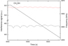 |
Fig. 1. Laser signals at two angles of incidence (left axis) and straight variation of the frequency of a QCMB (right axis) during methanol deposition at 80 K at constant rate. |
where λ0 is the wavelength of the He–Ne laser (633 nm), n0 is the refractive index of the ice film at the laser wavelength, and α the incidence angle of the laser from the surface normal. For most ices formed at low temperatures n0 is unknown. Two interference patterns were obtained at two different angles of incidence (34° and 64°, left axis Fig. 1), giving us a second equation to solve two unknowns. The refractive index can be obtained directly from
 (3)
(3)
where  and Tα and Tβ are the periods of the corresponding angles of incidence measured in seconds.
Films were formed at constant temperature allocating the QCMB at the end of the second stage of a Leybold closed-cycle He cryostat, where the temperature could be controlled from 12 K to room temperature by an ITC Oxford temperature controller. In these experiments, the temperature was fixed within 1 K. Cold parts were surrounded by a radiation shield inside a high vacuum chamber to prevent contaminants in the QCMB. The pressure in the chamber increases from 5 × 10⁻⁸ mbar before accretion to a constant value of 10−5 mbar during the deposition. Methanol molecules pass from a prechamber to the deposition chamber through a needle valve. Methanol pressure in the prechamber is maintained constant at 18.7 mbar thanks to both a liquid methanol reservoir at constant temperature and a controlled flux, through another needle valve, from the reservoir to the prechamber. These conditions lead to a deposition rate of ≈1 nm s−1. The methanol used was from Panreac, UHPLC, 99.9% purity, degasified previous to deposition.
Infrared spectra were obtained in the IEM-CSIC laboratory at Madrid. Ices of methanol were grown in a high vacuum 150 mm diameter cylindrical chamber pumped with a 210 l s−1 (for N2) turbo pump through a DN100 CF flange placed in its base. The chamber is provided with a closed-cycle He cryostat, coupled to a Fourier transform infrared spectrometer and a He–Ne laser to measure ice thickness by interferometry (see Fig. 2). The gas was introduced into the chamber through a needle valve coming from a methanol line (Fisher Scientific, HPLC, 99.99% purity) thermally stabilized at a vapour pressure of 40 ± 2 mbar. This low pressure was achieved and held constant immersing a methanol flask in an ice-water bath. The gas inlet is situated 120 mm below the optical axis transversal plane, and 200 mm above the pump flange. The geometry of the chamber was especially designed to obtain a symmetric deposition on both sides of the IR transparent Si wafer, placed in close contact with the cold head of the cryostat. This was confirmed by monitoring with the He–Ne laser the desorption of the back-side deposit. We found that we have the same thickness in both faces, within 5% error. For the experiments performed in this publication we employed a constant growth rate of 1.2 nm s−1, estimated using Eq. (2), and the time it takes to grow an interference maximum. At this growing rate, the water contamination of the methanol ice, due to the residual water vapour in the chamber, is less than 0.1%. The experiments were performed via the following sequence: first, the desired temperature was set; then gas was introduced in the chamber while He–Ne interference fringes were recorded; after one maximum of interference was grown, the gas inlet valve was closed, and a MIR spectrum was taken. This sequence was repeated until four interference maxima were grown and four MIR spectra were obtained. We note that it was necessary to rotate alternatively the Si substrate to face two different windows in the chamber to record He–Ne interferences in quasi normal incidence (4.0 ± 0.2°) or to take FTIR spectra in normal transmission configuration (see Fig. 2). Due to the weakness of the NIR absorptions, no NIR spectra were recorded for those thin layers. Subsequently, at the same temperature, ten more interference maxima were grown and, finally, a near infrared spectrum of the thick ice layer was obtained. Infrared spectra were recorded with a Burker Vertex 70 spectrometer, using a Globar source and a KBr beam splitter for the MIR spectral range, and a CaF beamspliter and a NIR lamp for the NIR range. The same mercury cadmium telluride detector was used for both regions. We worked at 2 cm−1 resolution and an accumulation of 300 scans. In these experiments, ice layer thicknesses were determined from He–Ne laser interference measurements, using Eq. (2) and n0 from Table 1. To avoid saturation of the MIR absorption bands, only ice layers up to ≈1000 nm thick were considered. In the NIR spectral range, ice layers of about 3400 nm were employed.
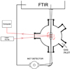 |
Fig. 2. Scheme of the experimental set-up used to record transmission IR spectra of methanol ices. |
2.1. Infrared optical constants
Infrared optical constants and refractive index are denoted in the following n(NIR)+i k(NIR) and n(MIR)+i k(MIR) respectively for the NIR and MIR spectral ranges. In this work we set the limits for the NIR region from 5000 (2.0 μm) to 3600 cm−1 (2.7 μm), and for the MIR region from 3600 (2.7 μm) to 650 cm−1 (15.4 μm). To determine n(MIR) and k(MIR) we have followed a procedure developed in our group and described in detail in Zanchet et al. (2013). This procedure takes advantage of the redundancy of information available when a set of spectra of different thicknesses of the same ice is available. In particular, four mid-IR spectra with thickness between 200 nm and 1000 nm were recorded for each ice. Theoretical transmission spectra were obtained using the Fresnel equations for a multilayer system vacuum/ice/silicon/ice/vacuum, and taking initial input values for n(MIR), k(MIR), n0 (visible refractive index), and L (ice layer thickness). Then the difference between experimental and theoretical spectra for the four experimental spectra available were minimized (see details in Zanchet et al. 2013). In the minimization procedure the measured n0 and layer thickness can vary within experimental error. Additionally, a coherence parameter that varies between 1 and 0 is fitted to consider coherence losses of the IR radiation in its transmission path through the layered system. At the end of the fitting procedure a set of n(MIR) and k(MIR) optical constants is obtained.
For the near infrared spectral range, infrared scattering and coherence losses become important in relation to the intensity of the absorptions, and the model described above, based on Fresnel equations, is not able to reproduce the experimental infrared interference pattern in the 5000–3500 cm−1 region. For this reason, we decided to record a single NIR spectrum for each ice temperature, corresponding to a thickness of about 3400 nm, and to extract k(NIR) applying Lambert–Beer’s law
 (4)
(4)
where Abs(μ) is the absorbance spectrum (baseline subtracted), L the ice thickness, and μ the frequency. The real component n(NIR) was then obtained by means of the Kramers–Kroning relation between n and k, considering the information we have for n0, n(MIR), and k(MIR).
Refractive index at 633 nm and densities of pure CH3OH ices grown at the indicated temperatures.
2.2. Band strengths
The integrated band strengths can be obtained from the imaginary part of the refractive index via
 (5)
(5)
where ρ is the ice density. Ice densities at different temperatures were taken from Table 1. When the imaginary part of the refractive index is not known it is possible to obtain an effective band strength, A′, from the absorbance spectrum and the column density of absorbing species, using
 (6)
(6)
The effective band strength can be affected by scattering and IR interferences that disturb the baseline of the absorption spectra and are difficult to disentangle form real absorptions (Hudson et al. 2014). It is interesting to point out that Eqs. (5) and (6) both involve the density of the ice. Ice densities are usually unknown and an A′ value is usually estimated assuming an ice density of 1 g cm−3. This was not the case in the present work, where we have measured the densities of the ices in an independent experiment (see Table 1).
3. Results
3.1. Densities and refractive indices.
Figure 3 collects density and refractive indices at eight temperatures covering the range from 20 to 130 K. Each experimental point is the result of two experiments except for 100 K, which corresponds to the mean value of eight different experiments. Experimental errors are calculated from the T-student with 95% confidence, from 12 experiments for T ≥ 100 K, and applied to the complete data set. This procedure gives errors of 0.01 g cm−3 for densities and 0.01 for the refractive indices.
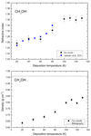 |
Fig. 3. Variation in density and refractive index of methanol with deposition temperature. |
The two parameters have the same general behaviour: ρ and n0 grow with the temperature of deposition from 20 K to 100 K. For higher temperatures both remain almost constant. The lower values correspond to 0.64 g cm−3 and 1.26 at 20 K, and the higher values to 0.813 g cm−3 and 1.344 for T ≥ 100 K. In the density plot we have indicated the value used in the bibliography for methanol, 1 g cm−3 (Hudgins et al. 1993; Maté et al. 2009; Bouilloud et al. 2015; Torrie et al. 1989).
Refractive indices vary from about 1.26 to 1.34. This last value is almost constant for T ≥ 100 K, matching the refractive index usually employed in the bibliography, 1.33 (Hudgins et al. 1993; Bouilloud et al. 2015), but disagreeing for lower temperatures of deposition (from 20 to 80 K). Our experimental refractive indices match those obtained by Isokoski et al. (2014; blue squares in Fig. 3). Both sets of experiments show increasing n0 values from 20 K to 100 K. In both cases the slope seems to vary depending on the deposition temperature. The lowest slope corresponds to temperatures ranging from 40 to 60 K. This seems to be similar to the values reported in Cazaux et al. (2015) for water ice simulations, and would be related to the number of neighbours a molecule is interacting with.
This overall behaviour is similar to that of other molecules studied before: CO2 (Satorre et al. 2008), NH3 (Satorre et al. 2013), and C2H4 and C2H6 (Satorre et al. 2017). An amorphous structure is formed at low temperature that increases its order with increasing deposition temperature until a maximum density (or refractive index) is achieved, corresponding to a crystalline structure. Methanol is atypical because this maximum (at 100 K) does not imply that the crystal is formed, as indicated by the IR spectra. These spectra reveal different crystalline structures at T ≥ 110 K, but its refractive indices and densities remain almost constant. The small variations in these values in Fig. 3 above 100 K are difficult to assign to structural changes within our error bars.
3.2. Infrared spectra
Figure 4 shows an example of the spectra obtained for methanol ices grown at eight different temperatures, from 20 K to 130 K. An adequate baseline has been subtracted. An amorphous solid is formed in deposits at temperatures equal to or below 100 K. At these temperatures the spectra have a similar shape, denoting the amorphous structure, although some differences can be appreciated. There is an overall tendency for all the bands to become narrower and to increase their maximum peak intensity values with increasing deposition temperature (see e.g. the band at 1027 cm−1). Interestingly, at higher wavenumbers the broad OH stretching band at 3250 cm−1 presents a shoulder for ices grown between 20 and 60 K which disappears at 80 K. The band is amplified in Fig. 5a. The presence of that shoulder at 3400 cm−1 might be correlated with the density of the ice (see Fig. 3) the spectral signature being larger for lower ice densities. A possible interpretation of these results, in connection with what is observed for water ice, could be the presence of pores in the amorphous methanol ice where methanol molecules are situated with weakly bonded O–H bond or even dangling bonds responsible of the larger wavenumber absorptions in the spectrum.
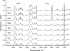 |
Fig. 4. Infrared spectra of methanol ices grown at the indicated temperatures. Appropriate baselines have been subtracted. The spectra correspond to layers about 990 nm thick. Spectral regions with weak absorptions have been multiplied by a factor indicated in the figure. Vertical offsets have been added to the absorbance spectra for clarity in the representation. |
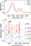 |
Fig. 5. Enlargement of part of the spectra presented in Fig. 4 to highlight (panel a) the shoulder at higher wavenumbers in the 3250 cm−1 band, and (panel b) the differences between compact-amorphous (100 K) and crystalline structures (110 K, 120 K, 130 K). |
Between 100 K and 110 K a phase transition from amorphous to polycrystalline solid is revealed by the strong changes that are observed in the IR spectra (see Fig. 5b). However, the crystalline form obtained at 110 K changes when the ice is deposited at 120 K and above. The intermediate phase at 110 K could be a different crystalline form or maybe just a mixture of amorphous and crystalline phases. Nonetheless, taking a closer look to the spectrum of the ice at 110 K, it is observed that there are already very sharp features at 4000 cm−1, 2950 cm−1, and 1450 cm−1, pointing to the presence of a crystalline form at 110 K. It is interesting to note here the result by Isokoski et al. (2014) that follows the interference signal of a He–Ne laser during thermal annealing of methanol ice grown at 20 K. They found an abrupt decay of the signal at about 100 K, which denotes a compaction of the ice before crystallization. This process of compaction but not crystallization agrees with what is observed in our experiments (see Figs. 3–5).
We have also followed the infrared spectral changes of an ice upon annealing at 5 K min−1 from 20 K to 130 K. Figure 6 shows two absorption regions chosen to illustrate the differences in the spectra due to the different degrees of crystallization obtained by direct deposition (left panel) or thermal annealing (right panel). At 110 K, 120 K, and 130 K the crystalline ice obtained by annealing does not reach the degree of crystallinity that the ices grown by direct vapour deposition have at thdse same temperatures.
 |
Fig. 6. Infrared spectra of methanol ices grown at the indicated temperatures (left panels) or grown at 20 K and annealed to the indicated temperatures (right panels). Appropriate baselines have been subtracted. The spectra correspond to layers about 990 nm thick. Vertical offsets have been added to the absorbance spectra for clarity in the representation. |
3.3. Optical constants and band strengths
The NIR and MIR optical constants of solid methanol obtained in this work by the procedure described in Sect. 2.1 are presented in Fig. 7. It is important to remember that for the determination of these magnitudes from the IR spectra it is not necessary to know the ice densities, only the thickness of the ice layers. At the end of the iterative procedure, the simulated spectra reproduce the experimental observations with a root mean square deviation of 0.001 in absorbance units. We estimate overall uncertainties of ≈1% for the real component of the refractive index n. The uncertainty is also ≈1% for the imaginary component, k, except when k < 0.01, which induces larger errors due to the higher signal-to-noise ratio in the film-substrate transmittance.
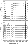 |
Fig. 7. Infrared real (n) and imaginary (k) part of the refractive index of methanol ices at different deposition temperatures. Vertical offsets have been added to the magnitudes for clarity in the representation. In the lower panel, k multiplied by 50 has been represented in the 3700 and 5000 cm−1 spectral range. |
In Tables 2 and 3 we present the NIR and MIR band strengths obtained in this work at different temperatures for amorphous and crystalline ices, respectively. Mode assignments are presented in the first two columns. In the third column peak positions are listed, although for most cases several unresolved peaks are present in the integration region, and these positions are somewhat arbitrary. The fourth column indicates the integration intervals employed. We have estimated the absolute band strengths, A, and the effective band strengths, A′, in the MIR region using the expressions in Eqs. (5) and (6), respectively. In the NIR spectral range the two magnitudes coincide since the k values were obtained after subtracting a baseline and applying the Lambert–Beer law. The ice densities needed were taken from Table 1. An average experimental error of 20% was estimated for theses magnitudes, being smaller for the stronger features and larger for the weaker ones. This error is mostly due to the criteria used to choose the integration intervals.
In Fig. 8 we have represented the evolution of the band strengths with temperature for two bands. It can be seen that the band strengths do not change appreciably, within experimental error, for temperatures below 100 K. However, some modifications are observed when the ice phase changes from amorphous to crystalline above 100 K. These findings are in good agreement with those of Kerkhof et al. (1999), where no variation was found for the band strength of pure methanol ices grown at 10 K and annealed up to 100 K. In that work, higher temperatures were not investigated for the pure species. At higher temperatures, the observed changes point to the different crystalline structures formed by deposition at 110 K, 120 K, or 130 K.
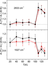 |
Fig. 8. Temperature dependence of methanol IR band strengths at 2833 cm−1 and 1027 cm−1. The two sets of data represented correspond to A (open red circles) and A′ (solid black circles). |
Absolute (A) and effective (A′) band strengths of CH3OH amorphous ice grown at the indicated temperatures.
Absolute (A) and effective (A′) band strengths of CH3OH crystalline ice grown at the indicated temperatures.
4. Discussion
To our knowledge the article Hudgins et al. (1993; hereafter HSAT) presents the most complete set of IR data of pure methanol ice published so far. In particular, they provide the only set of optical constants reported for pure solid methanol in the MIR range. These authors studied a methanol ice grown at 10 K and annealed to higher temperatures. In Fig. 9 we compare the optical constants we obtained for methanol ice at 20 K to those by HSAT at 10 K. It can be seen that the literature values are higher and they approach our data if they are scaled by a factor 0.64. This factor is close to the density we measured for methanol ice at low temperature (see Table 1).
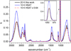 |
Fig. 9. Comparison of the imaginary part of the refractive index of solid methanol ice at 20 K provided in this work (black) with the values reported by Hudgins et al. (1993; blue). The scaled literature values are represented with a dashed red line. |
Although the imaginary part of the refractive index, k, as a characteristic of the solid depends on its density, it can be determined without the knowledge of that magnitude. The only ice parameter needed for calculating k is the visible refractive index of the ice, n0, which is needed to obtain the ice layer thickness from Eq. (2). The refractive index assumed in HSAT for methanol ice was 1.33, taken from the value for liquid CH3OH given by Weast (1972). The refractive index we have measured for methanol at 20 K in this work is 1.26. From this data, the ice film thickness considered by HSAT could be underestimated. However, it is likely that the ice grown by HSAT at 10 K will not have the same n0 or density as the ice grown at 20 K in our work. In their experiments the gas was introduced into the vacuum chamber though a tube directed perpendicular to the cold substrate, while in our work the whole vacuum chamber was filled with a homogenous pressure of methanol gas (background deposition). Random-trajectory background deposition generates more porous ices than directional deposition (Dohnálek et al. 2003; Bossa et al. 2015). Therefore, it is expected that the methanol ice grown by HSAT at 10 K is more compact than the ice grown in the present work at 20 K. A smaller number of absorbers, related to the large porosity of our samples, will be evidenced as a decrease in the imaginary part of the refractive index. On the contrary, a more compact ice will absorb more IR radiation, which means higher k values. These considerations are in agreement with the scaling factor applied to match the two sets of k values represented in Fig. 9. Apart from the overall scaling factor, differences in the shape and relative intensities of some features of the two sets of optical constants can be seen, mostly above 100 K. In Fig. 10 the k values given by HSAT at different temperatures are compared to our data for the bands at ≈2833 cm−1 (3.53 μm) and at ≈1027 cm−1 (9.74 μm), two of the peaks most widely employed for methanol identification in astrophysical media. The literature data in Fig. 10 have been scaled for clarity. There is very good agreement in the shape of the two sets of constants for amorphous samples from 10 K up to 100 K (see the four lower lines in both panels). However, the differences in shape are significant between the k values reported in HSAT for crystalline ice at 120 K and the three sets of constants at 110 K, 120 K, and 130 K reported in this work (see the four upper lines in both panels). This situation shows that the structure obtained by direct deposition is more ordered than that obtained by an ice deposited at low temperature and annealed.
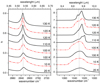 |
Fig. 10. Comparison between k values from this work (solid black lines) and those from Hudgins et al. (1993; dashed red lines). Literature data have been scaled for clarity in the representation. Vertical offsets have been added to the magnitudes for the same purpose. |
Different band strengths for CH3OH ice at low temperature reported in the literature are compared with our data in Table 4. The A′ estimated by HSAT assuming an ice density of 1 g cm−3 coincides with our data. As commented above, we believe HSAT methanol ice is denser than that grown in this work, and its density could be close to 1 g cm−3. It could be the case that the actual density of their ice is lower. The agreement found could then be explained by an underestimation of their ice layer thickness values, since this would lead to a similar number of absorbers (molecules cm−2). It can be seen in the fourth column of Table 4 that correcting HSAT A′ values considering the methanol ice density measured in this work, 0.64 g cm−3 at 20 K, leads to a large disagreement. In the last column of Table 4 the results of a recent work by Bouilloud et al. (2015) are presented. They correspond to band strengths of methanol ice grown at 25 K by deposition through a capillary that is 10 cm away from the cold surface, with an incidence angle of 45°. This could be considered similar to background deposition and the ice could have low density, 0.64 g cm−3, like those grown in the present work at 20 K. When the values presented in Bouilloud et al. (2015) are corrected assuming an ice density of 0.64 g cm−3, they coincide very well with our data.
Absolute band strengths (× 1018 cm molecule−1).
5. Conclusions
We have measured new densities, ρ, visible refractive indices at 633 nm, n0, IR optical constants, and IR band strengths for methanol ices grown by vapour deposition at 20 K, 40 K, 60 K, 80 K, 100 K, 110 K, 120 K, and 130 K.
Methanol-ice densities and visible refractive indices increase with the temperature of deposition in the interval 20–100 K. They remain almost constant from 100 K to 130 K, which is the highest temperature investigated. The growth is sharper for the interval 60–100 K, in agreement with the n0 values obtained by Isokoski et al. (2014) in similar accretion conditions. The refractive index does not vary between 40 and 60 K, a behaviour that resembles that obtained by Cazaux et al. (2015) for water ices.
Methanol-ice grown at 100 K presents an anomalous behaviour. It acquires an amorphous structure as dense as the crystalline form. This was revealed by looking at our density and infrared spectra measurements. This particularity has not been observed for any other molecular ice previously studied in our laboratory. For example, CO2, C2H6, C2H4, and NH3 ices have a lower density in amorphous phases than in crystalline phases. This finding coincides with the sudden ice compaction that takes place at 100 K for CH3OH ice when deposited at 20 K and warmed up as shown in Isokoski et al. (2014). This compaction is not associated with crystallization either, as shown by infrared spectroscopy when annealing CH3OH to 100 K.
Infrared spectra of crystalline methanol obtained by annealing ices grown at 20 K to 110 K, 120 K, and 130 K show that they are different to the crystalline ices obtained by direct vapour deposition at these temperatures. Optical constants in the NIR and MIR spectral ranges, from 5000 cm−1 to 650 cm−1, are provided for amorphous and crystalline methanol ices grown at eight temperatures from 20 K to 130 K. These optical constants differ from the Hudgins et al. (1993) data, due to the different ice-generation conditions which lead to different morphologies and phases.
We also present methanol band strengths in the NIR and MIR spectral ranges at the same eight temperatures mentioned above. Some band strengths vary for crystallized ices up to 30%. This temperature dependence must be considered to properly estimate the amount of methanol in different astrophysical environments.
For low temperature band strengths, we have compared our results with previous literature data collected by Bouilloud et al. (2015). We found that at low temperatures (10 K–25 K), methanol band strengths do not depend appreciably on the ice morphology, but only on the number of absorbers. Therefore, all the literature data agree if the adequate ice densities, which depend on the generation conditions, are taken into account. Our measurements allowed us to explain discrepancies of about 40% in some band strengths previously reported by Bouilloud et al. (2015).
The spectral shape of the different features in the infrared spectra of methanol ices are distinctive and can help to trace the phase and temperature of methanol ices detected in the ISM or in different solar system objects, and will give information about the formation history of the ices observed.
Acknowledgments
Funds have been provided for this research by the Spanish MINECO, Project FIS2016-77726-C3-1-P and FIS2016-77726-C3-3-P. Germán Molpeceres acknowledges MINECO PhD grant BES-2014-069355. We are grateful to R. Escribano for helpful discussions. Our skillful technicians C. Santonja, M. A. Moreno, and J. Rodríguez are also gratefully acknowledged.
References
- Boogert, A. C. A., Pontoppidan, K. M., Knez, C., et al. 2008, ApJ, 678, 985 [NASA ADS] [CrossRef] [Google Scholar]
- Boogert, A., Gerakines, P., & Whittet, D. 2015, ARA&A, 53, 541 [Google Scholar]
- Bossa, J.-B., Maté, B., Fransen, C., et al. 2015, ApJ, 814, 47 [NASA ADS] [CrossRef] [Google Scholar]
- Bottinelli, S., Boogert, A. C., Bouwman, J., et al. 2010, ApJ, 718, 1100 [NASA ADS] [CrossRef] [Google Scholar]
- Bouilloud, M., Fray, N., Bénilan, Y., et al. 2015, MNRAS, 451, 2145 [NASA ADS] [CrossRef] [Google Scholar]
- Cazaux, S., Bossa, J.-B., Linnartz, H., & Tielens, A. G. G. M. 2015, A&A, 573, A16 [NASA ADS] [CrossRef] [EDP Sciences] [Google Scholar]
- Dartois, E., Schutte, W. A., & Geballe, T. R. 1999, A&A, 342, L32 [NASA ADS] [Google Scholar]
- d’Hendecourt, L. B., & Allamandola, L. J. 1986, A&AS, 64, 453 [NASA ADS] [Google Scholar]
- Dohnálek, Z., Kimmel, G. A., Ayotte, P., Smith, R. S., & Kay, B. D. 2003, J. Chem. Phys., 118, 364 [NASA ADS] [CrossRef] [Google Scholar]
- Drabek-Maunder, E., Greaves, J., Fraser, H. J., Clements, D. L., & Alconcel, L. N. 2017, Int. J. Astrobiol., DOI: 10.1017/S1473550417000428 [Google Scholar]
- Gálvez, O., Maté, B., Martín-Llorente, B., Herrero, V. J., & Escribano, R. 2009, J. Phys. Chem. A, 113, 3321 [CrossRef] [Google Scholar]
- Gerakines, P. A., Bray, J. J., Davis, A., & Richey, C. R. 2005, ApJ, 620, 1140 [NASA ADS] [CrossRef] [Google Scholar]
- Hodyss, R., Parkinson, C. D., Johnson, P. V., et al. 2009, Geophys. Res. Lett., 36, 2 [CrossRef] [Google Scholar]
- Hudgins, D. M., Sandford, S. A., Allamandola, L. J., & Tielens, A. G. G. M. 1993, ApJS, 86, 713 [NASA ADS] [CrossRef] [Google Scholar]
- Hudson, R., Ferrante, R., & Moore, M. 2014, Icarus, 228, 276 [Google Scholar]
- Ioppolo, S., van Boheemen, Y., Cuppen, H. M., van Dishoeck, E. F., & Linnartz, H. 2011, MNRAS, 413, 2281 [NASA ADS] [CrossRef] [Google Scholar]
- Isokoski, K., Bossa, J.-B., Triemstra, T., & Linnartz, H. 2014, Phys. Chem. Chem. Phys., 16, 3456 [NASA ADS] [CrossRef] [Google Scholar]
- Kerkhof, O., Schutte, W., & Ehrenfreund, P. 1999, A&A, 346, 990 [NASA ADS] [Google Scholar]
- Maté, B., Gálvez, Ó., Herrero, V. J., & Escribano, R. 2009, ApJ, 690, 486 [NASA ADS] [CrossRef] [Google Scholar]
- Merlin, F., Quirico, E., Barucci, M. A., & de Bergh, C. 2012, A&A, 544, A20 [NASA ADS] [CrossRef] [EDP Sciences] [Google Scholar]
- Molpeceres, G., Satorre, M. A., Ortigoso, J., et al. 2016, ApJ, 825, 156 [NASA ADS] [CrossRef] [Google Scholar]
- Öberg, K. I. 2016, Chem. Rev., 116, 9631 [Google Scholar]
- Palumbo, M. E., Castorina, A. C., & Strazzulla, G. 1999, A&A, 342, 551 [NASA ADS] [Google Scholar]
- Pontoppidan, K. M., Dartois, E., van Dishoeck, E. F., Thi, W.-F., & D’Hendecourt, L. 2003, A&A, 404, L17 [NASA ADS] [CrossRef] [EDP Sciences] [Google Scholar]
- Sandford, S. A., & Allamandola, L. J. 1993, ApJ, 417, 815 [NASA ADS] [CrossRef] [PubMed] [Google Scholar]
- Satorre, M., Domingo, M., Millán, C., et al. 2008, Plan. Spa. Sci., 56, 1748 [NASA ADS] [CrossRef] [Google Scholar]
- Satorre, M., Leliwa-Kopystynski, J., Santonja Molté, C., & Luna, R. 2013, Icarus, 225, 703 [NASA ADS] [CrossRef] [Google Scholar]
- Satorre, M., Millán, C., Molpeceres, G., et al. 2017, Icarus, 296, 179 [NASA ADS] [CrossRef] [Google Scholar]
- Sauerbrey, G. 1959, Z. Phys., 155, 206 [Google Scholar]
- Torrie, B. H., Weng, S. X., & Powell, B. M. 1989, Mol. Phys., 67, 575 [NASA ADS] [CrossRef] [Google Scholar]
- Watanabe, N., & Kouchi, A. 2002, ApJ, 571, 173 [Google Scholar]
- Weast, R. 1972, Handbook of Chemistry and Physics, 53rd edn. (Cleveland: Chemical Rubber Co.), 155 [Google Scholar]
- Zanchet, A., Rodríguez-Lazcano, Y., Gálvez, Ó., et al. 2013, ApJ, 777, 26 [NASA ADS] [CrossRef] [Google Scholar]
All Tables
Refractive index at 633 nm and densities of pure CH3OH ices grown at the indicated temperatures.
Absolute (A) and effective (A′) band strengths of CH3OH amorphous ice grown at the indicated temperatures.
Absolute (A) and effective (A′) band strengths of CH3OH crystalline ice grown at the indicated temperatures.
All Figures
|
Fig. 1. Laser signals at two angles of incidence (left axis) and straight variation of the frequency of a QCMB (right axis) during methanol deposition at 80 K at constant rate. |
| In the text | |
|
Fig. 2. Scheme of the experimental set-up used to record transmission IR spectra of methanol ices. |
| In the text | |
|
Fig. 3. Variation in density and refractive index of methanol with deposition temperature. |
| In the text | |
|
Fig. 4. Infrared spectra of methanol ices grown at the indicated temperatures. Appropriate baselines have been subtracted. The spectra correspond to layers about 990 nm thick. Spectral regions with weak absorptions have been multiplied by a factor indicated in the figure. Vertical offsets have been added to the absorbance spectra for clarity in the representation. |
| In the text | |
|
Fig. 5. Enlargement of part of the spectra presented in Fig. 4 to highlight (panel a) the shoulder at higher wavenumbers in the 3250 cm−1 band, and (panel b) the differences between compact-amorphous (100 K) and crystalline structures (110 K, 120 K, 130 K). |
| In the text | |
|
Fig. 6. Infrared spectra of methanol ices grown at the indicated temperatures (left panels) or grown at 20 K and annealed to the indicated temperatures (right panels). Appropriate baselines have been subtracted. The spectra correspond to layers about 990 nm thick. Vertical offsets have been added to the absorbance spectra for clarity in the representation. |
| In the text | |
|
Fig. 7. Infrared real (n) and imaginary (k) part of the refractive index of methanol ices at different deposition temperatures. Vertical offsets have been added to the magnitudes for clarity in the representation. In the lower panel, k multiplied by 50 has been represented in the 3700 and 5000 cm−1 spectral range. |
| In the text | |
|
Fig. 8. Temperature dependence of methanol IR band strengths at 2833 cm−1 and 1027 cm−1. The two sets of data represented correspond to A (open red circles) and A′ (solid black circles). |
| In the text | |
|
Fig. 9. Comparison of the imaginary part of the refractive index of solid methanol ice at 20 K provided in this work (black) with the values reported by Hudgins et al. (1993; blue). The scaled literature values are represented with a dashed red line. |
| In the text | |
|
Fig. 10. Comparison between k values from this work (solid black lines) and those from Hudgins et al. (1993; dashed red lines). Literature data have been scaled for clarity in the representation. Vertical offsets have been added to the magnitudes for the same purpose. |
| In the text | |
Current usage metrics show cumulative count of Article Views (full-text article views including HTML views, PDF and ePub downloads, according to the available data) and Abstracts Views on Vision4Press platform.
Data correspond to usage on the plateform after 2015. The current usage metrics is available 48-96 hours after online publication and is updated daily on week days.
Initial download of the metrics may take a while.