| Issue |
A&A
Volume 691, November 2024
|
|
|---|---|---|
| Article Number | A306 | |
| Number of page(s) | 8 | |
| Section | Astrophysical processes | |
| DOI | https://doi.org/10.1051/0004-6361/202450097 | |
| Published online | 20 November 2024 | |
Infrared spectra of solid-state ethanolamine: Laboratory data in support of JWST observations
1
Max Planck Institute für Astronomie, Königstuhl 17, 69117 Heidelberg, Germany
2
Laboratory Astrophysics Group of the Max Planck Institute for Astronomy at the Friedrich Schiller University Jena, Institute of Solid State Physics, Helmholtzweg 3, 07743 Jena, Germany
⋆ Corresponding author; This email address is being protected from spambots. You need JavaScript enabled to view it.
Received:
22
March
2024
Accepted:
14
October
2024
Abstract
Context. Ethanolamine (NH2CH2CH2OH; EA) has been identified in the gas phase of the interstellar medium within molecular clouds. Although EA has not been directly observed in the molecular ice phase, a solid-state formation mechanism has been proposed. However, the current literature lacks an estimation of the infrared band strengths of EA ices, which are crucial data for quantifying potential astronomical observations and laboratory findings related to their formation or destruction via energetic processing.
Aims. We conducted an experimental investigation of solid EA ice at low temperatures to ascertain its infrared band strengths, phase transition temperature, and multilayer binding energy. Since the refractive index and the density of EA ice are unknown, the commonly used laser interferometry method was not applied. Infrared band strengths were determined using three distinct methods. In addition to evaluating EA band strengths, we also tested the advantages and disadvantages of different approaches used for this purpose. The obtained lab spectrum of EA was compared with the publicly available MIRI MRS James Webb Space Telescope observations towards a low-mass protostar.
Methods. We used a combination of Fourier-transform transmission infrared spectroscopy and quadrupole mass spectrometry.
Results. The phase transition temperature for EA ice falls within the range of 175 to 185 K. Among the discussed methods, the simple pressure gauge method provides a reasonable estimate of band strength. We derived a band strength value of about 1 × 10⁻¹⁷ cm molecule−1 for the NH2 bending mode in the EA molecules. Additionally, temperature-programmed desorption analysis yielded a multilayer desorption energy of 0.61±0.01 eV. By comparing the laboratory data documented in this study with the JWST spectrum of the low-mass protostar IRAS 2A, an upper-limit for the EA ice abundances was derived.
Conclusions. This study addresses the lack of quantitative infrared measurements of EA at low temperatures, crucial for understanding EA’s astronomical and laboratory presence and formation routes. Our approach presents a simple yet effective method for determining the infrared band strengths of molecules with a reasonable level of accuracy.
Key words: astrochemistry / methods: analytical / methods: laboratory: solid state / techniques: spectroscopic / ISM: molecules
© The Authors 2024
 Open Access article, published by EDP Sciences, under the terms of the Creative Commons Attribution License (https://creativecommons.org/licenses/by/4.0), which permits unrestricted use, distribution, and reproduction in any medium, provided the original work is properly cited.
This article is published in open access under the Subscribe to Open model.
Open access funding provided by Max Planck Society.
1. Introduction
Aminoalcohols are an interesting class of organic compounds that contain both amino (NH2) and hydroxy (OH) functional groups. These molecules, due to their biological relevance, can play an important role in the context of the origin of life. Ethanolamine (NH2CH2CH2OH; EA), also known as β-aminoethanol or glycinol, is the simplest head group of phospholipids and is also considered a precursor of the simplest amino acid, glycine. Additionally, α, β-amino alcohol moieties can be found in various other biomolecules, including aminosugars, sphingolipids, and glycoproteins, playing crucial roles in the functions of biosystems (Sladkova et al. 2014).
Recently, EA was identified in the interstellar medium in the molecular cloud G+0.693−0.027, situated within the Sagittarius B2 complex in the Galactic centre, through rotational transition observations as reported by Rivilla et al. (2021). Although EA was observed exclusively in the gas phase and not within interstellar ices, it has been proposed that the gas-phase detection may be attributed to the erosion of icy mantles caused by the low-velocity shocks typically found in massive molecular clouds. EA has also been found in the Almahata Sitta meteorite (Glavin et al. 2010).
One of the potential pathways for the formation of EA in space is through the hydrogenation of the aminoketene molecule (Rivilla et al. 2021). In a recent study, aminoketene was shown to be formed efficiently at 10 K without the input of energy by the reaction of C atoms with CO and NH3, which could potentially result in high abundances of aminoketene and EA in the solid state (Krasnokutski 2021; Krasnokutski et al. 2022). Aminoketene may also polymerize, resulting in the formation of peptide chains that could potentially have a catalytic function, aiding the formation of complex organic or even biological molecules (Krasnokutski et al. 2024, 2022). This pathway begins with the reaction between C and NH3 leading to the formation of HCNH2 and H2CNH products. This differs from a recently published work, which proposes that the reaction of C atoms with an NH3 molecule in ice forms a weakly bound complex, namely CNH3 (Molpeceres et al. 2024).
An alternative route to EA is the UV irradiation of molecular ice as demonstrated by laboratory experiments on the photolysis of H2O:CH3OH:NH3:HCN ices, with a 20:2:1:1 mixture (Bernstein et al. 2002). In these experiments, EA was produced along with other prebiotic species like the amino acids glycine, alanine, and serine. However, the amount of EA formed in these experiments was very small and it was detected after a chemical treatment. Therefore, the presence of EA, with its multiple functional groups, in molecular ice could lead to the formation of more complex species when exposed to energetic processing, some of which might even have astrobiological significance.
Infrared (IR) spectroscopy stands out as the primary method for identifying molecules in extraterrestrial solids, particularly in ice on interstellar and solar system objects. The identification process involves comparing astronomical data to reference measurements from terrestrial laboratories and, in some cases, allows for both identification and quantification of molecular abundances based on IR detections. This method relies on assigning specific IR bands to molecules, integrating them, and comparing the results to intrinsic IR band strengths determined in laboratories.
To our knowledge, there are no quantitative IR measurements of EA ices. This study concentrates on conducting IR spectroscopy on amorphous EA ice at low temperatures and assigning the IR bands based on theoretical calculations. The thermal variation of EA IR features is also shown. The phase transition temperatures have been identified and the IR spectra of crystalline EA have been highlighted. In addition, experimental band strengths of amorphous EA ice have been determined.
2. Experimental methods
Experiments were conducted in the Laboratory Astrophysics group at Jena in the INterStellar Ice Dust Experiment (INSIDE) chamber. The setup has been extensively detailed in prior work (Potapov et al. 2019). Here, we provide only a brief overview of the setup as relevant to this study. The measurements were done in an ultrahigh vacuum (UHV) chamber, maintaining a base pressure better than 8 × 10⁻¹⁰ mbar, which is equipped with a closed-cycle helium cryostat that can cool the sample down to 10 K. The temperature was measured by a diode fixed on the sample holder very close to the sample. In our experiments, a potassium bromide (KBr) window was affixed as a substrate on the cold finger of the cryostat.
Liquid NH2CH2CH2OH (Sigma Aldrich, ≥99.0%) and CH3OH (Sigma Aldrich, ≥99.0%) were purified through multiple freeze-pump-thaw cycles and deposited onto the substrate as pure vapour through a gas inlet system attached to the UHV chamber in different experiments. The gas inlet system has two separate lines. The first line allows mixing of up to five different gases. NH2CH2CH2OH and CH3OH were deposited individually from the first line. The second gas line is kept for corrosive gases. Ammonia (NH3, Linde, 5.5 grade purity) gas was also deposited as a pure component through the second gas line of the same inlet system without any further purification. Gases are deposited onto the substrate through two 0.5 mm diameter capillary tubes. The chamber is equipped with a Fourier transform IR (FTIR) spectrometer (Bruker Vertex 80v) fitted with a mercury cadmium telluride (MCT) detector for in situ measurement of the ice phase. IR spectra were collected in the temperature interval between 10 and 300 K, before and during the warming-up, in transmittance mode in the spectral range from 6000 to 400 cm−1 with a resolution of 1 cm−1. For the irradiation experiment at 10 K, 256 scans were taken, whereas during the warming-up experiment, only 32 scans were taken each time.
During the low-temperature and warming-up experiments, a quadrupole mass spectrometer (QMS; HXT300M, Hositrad) attached to the UHV chamber monitors the gas phase inside the chamber to detect molecules desorbing from the sample surface. Temperature programmed desorption (TPD) experiments were performed by linear ramping of the sample temperature with a rate of 10 K minute−1 in a temperature range between 10 and 300 K. The error of the temperature measurements was determined to be ±1 K.
The molecular geometry and anharmonic vibrational spectrum of one of the conformers of EA were obtained using the second-order Møller-Plesset (MP2) perturbation theory and Aug-cc-pVTZ basis set. Quantum chemical calculations were performed using the Gaussian09 software package (Frisch et al. 2016).
3. Results and discussion
3.1. IR spectrum of EA ice
Experimental IR spectra of EA in both its liquid and the gas phases have been reported in the literature (Silva et al. 1999, and references therein). Additionally, the adsorption behaviour of EA on TiO2 at temperatures of 35° and 275°C has been investigated (Tseng et al. 2010). However, to date, a comprehensive study of EA ices at low temperatures has not been conducted. Matrix-isolated IR spectra of EA at 13 K were measured in the laboratory, focusing only on the spectral regions between 3800−3300 and 600−200 cm−1 (Räsänen et al. 1983). Figure 1 illustrates the IR spectrum of EA deposited on a blank KBr substrate at 10 K. To aid in the assignment of the fundamental vibration modes associated with this spectrum, a fully anharmonic IR spectrum of a single EA molecule was computed. The computed IR spectrum is also shown in Fig. 1. Since the formation of ice significantly alters the spectrum of EA, especially in the stretching vibration region, the assignment of absorption bands is also based on previous laboratory data and is shown in Table 1. Although the computed spectrum agrees well with the experiment in the fingerprint region (i.e. low wavenumber side), there are a few discrepancies on the higher wavenumber side. Notably, the O-H stretching band of EA in the experiment deviates significantly from results obtained using computations. The possible cause of deviation is the presence of an extended H-bond network that exists in EA ice which was not considered for free hydroxy and amino groups in the computation.
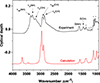 |
Fig. 1. Experimental and theoretical mid-IR spectrum of EA. The upper one shows about 200 monolayers (ML) of EA condensed on KBr at 10 K. The IR bands marked with asterisks are due to a mixture of different vibrational modes. For the latter, calculations were performed at MP2/Aug-cc-pVTZ level. |
IR band positions of EA from experiment and calculation.
3.2. Thermal variation of IR spectrum of EA ice
A pure EA ice grown at 10 K was heated with a continuous linear ramp of 10 K min−1 up to 140 K. The spectral changes were monitored with FTIR. After 140 K, the sample was heated in increments of 5 K with the same ramp. After reaching each heating step, heating was paused for an IR measurement and then resumed until a final temperature of 250 K was reached. While the phase transition was observed between 175 and 185 K, EA sublimation started at 220 K, well above the water sublimation temperature, and continued until 240 K. The reproducibility was confirmed through a subsequent experiment. It is worth mentioning at this point that the maximum desorption temperature for the EA multilayer (about 200 monolayers; ML) is 40 K higher than that measured for small coverages (a few ML) by the TPD method described in the next section. Figure 2 shows the spectra at different temperatures during the annealing process of EA.
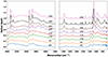 |
Fig. 2. Series of mid-IR spectra of EA shown at different temperatures and two different spectral regions. About 200 ML of EA were initially condensed on the KBr surface at 10 K and warmed up to 250 K with a linear heating ramp. Spectra are shifted in ordinate for clarity. The spectrum at 190 K is made bold to indicate the complete phase transition from amorphous to crystalline. |
The features of interest are mostly located within these two ranges: 3600−2500 cm−1 and 1600−800 cm−1. For the higher wavenumber range, the band observed at 3351 cm−1, associated with asymmetric NH2 stretching, sharpened with increasing temperature, and the peak was eventually red-shifted to 3338 cm−1 at 145 K. The band then remained unchanged until 170 K. During the phase transition, the 3338 cm−1 band began to disappear and was replaced by a sharp 3322 cm−1 band. With further temperature increase, the 3322 cm−1 band blue-shifted to 3327 cm−1 until the complete desorption of EA. Meanwhile, the band at 3286 cm−1, ascribed to symmetric NH2 stretching, grew sharper until the sample reached 175 K but without a change in the peak position. During the phase transition, the 3286 cm−1 vanished and a new band centred at 3271 cm−1 appeared. The band assigned to OH stretching at 3185 cm−1 blue-shifted to 3200 cm−1 and grew sharper up to 180 K. Beyond that, the 3200 peak started to disappear and a new band was formed at 3182 cm−1, which was closer to the original band but better resolved. A shoulder peak at 3055 cm−1 on the lower wavenumber side of the OH stretching band becomes prominent while heating the ice beyond 100 K. The peak then remained unchanged until 175 K before broadening. For the asymmetric CH2 stretching band at 2928 cm−1, although no change in the peak position was observed, the peak became sharper by heating up to 175 K. After this, the peak started to disappear and instead, a new band was formed with a peak centred at 2939 cm−1. On the other hand, a symmetric CH2 stretch band at 2857 cm−1 shifted up to 2864 cm−1 at 170 K. The peak then disappeared and also formed a new band with a peak at 2875 cm−1. Apart from the bands mentioned in Table 1, there were a few small peaks centred around 2777 cm−1, 2718 cm−1 and 2653 cm−1 observed at 10 K which remained at the same position even after annealing until 170 K. All these peaks resolved upon annealing and show a considerable shift of up to 15 cm−1 beyond 180 K. Two new peaks appeared in the EA ice spectrum beyond 180 K at 2565 cm−1 and 2522 cm−1. Close to the desorption temperature, the 2565 cm−1 disappeared while the 2522 cm−1 peak shifted to 2510 cm−1.
Simultaneously, for the lower wavenumber range, the 1607 cm−1 band assigned to NH2 bending shows no change in peak position until about 175 K. Between 175 and 185 K, 1607 cm−1 peak disappeared and instead, two new features appeared – a strong band at 1614 cm−1 and a weak band at 1668 cm−1. Similarly, the 1458 cm−1 peak assigned to CH2 bending gradually smeared out until 175 K, and beyond that, during the phase transition, it formed a strong band at 1486 cm−1 and a weak band at 1450 cm−1. We also noticed a peak emerging at 1467 cm−1 which eventually became a shoulder to the 1486 cm−1 peak. The 1395 cm−1 band shows almost no change in the peak position until 175 K, while between 175 and 185 K, the peak shifted to 1380 cm−1. On the other hand, 1360 cm−1 peak became sharp but remained around 1357 cm−1 until 175 K; beyond that the peak split into a strong 1346 cm−1 and a weak 1366 cm−1. After 185 K, both the peaks started to disappear gradually. The 1253, 1175, 1082, and 1033 cm−1 bands show no change in the peak position until 175 K. During the phase transition, we saw the peak shifting to 1160 cm−1 in the case of 1175 cm−1 band, while the 1082 and 1033 cm−1 bands show splitting to 1100 and 1063 cm−1 peaks for the former and 1038 and 1030 cm−1 peaks for the latter. Two new peaks at 970 and 1313 cm−1 started to appear as we began to heat the EA ice and remained unchanged until 175 K. During the phase transition, the 970 cm−1 peak split into 982 and 960 cm−1 peaks. After 185 K, a new peak appeared at 870 cm−1.
3.3. Band strength estimation
In the laboratory, optical laser interferometry is frequently paired with complementary techniques to determine the IR band strengths of solid molecules (Bouilloud et al. 2015; Hudson et al. 2022, and references therein). The precise estimation of absolute band strengths relies on prior knowledge of the refractive index and density of the molecule under study, which laser techniques can help with. In the present work, we have determined the IR band strengths of EA by three different methods, none of which involve laser interferometry. The band strengths derived by the first two methods require comparison of the absorption spectra of molecules with known reference band strengths, whereas for the last method, no such comparison is required.
IR band strength (A, cm molecule−1) of any absorption band of a molecule is given by:
 (1)
(1)
where N is the column density of the molecule in molecules cm−2, τ the optical depth of the absorption band (unitless), and ν the wavenumber frequency in cm−1. To determine the band strength, the column density of the molecule has to be measured. In the case of the first method, we considered that the column density will depend on the gas pressure difference (Δp) measured in the gas inlet system during the molecule deposition. The pressure difference was measured via the capacitance diaphragm vacuum gauge (Pfeiffer Vacuum, CCR 364). The gas pressure obtained this way is independent of the gas type and the concentration. Therefore, assuming an ideal gas equation and considering that all the other parameters remain unchanged from one measurement to the other, N would be proportional to Δp in the gas inlet system. A similar dependence has been shown previously (González Díaz et al. 2022). For this method of band strength estimation of EA, we use a reference molecule and re-arrange Eq. (1) as the following:
 (2)
(2)
The integrated band areas for EA and the reference molecules were evaluated from the IR spectra. We used CH3OH and NH3 as reference molecules. The bands of CH3OH and NH3 selected for the integrated optical depth estimations are shown with shaded regions in Fig. 3, and the respective absolute band strengths are listed in Table 2. In the case of NH3’s 1071 cm−1 peak, the absolute band strength was calculated using the imaginary part of the optical constants k(ν) given as a function of wavenumbers that was obtained from NASA Cosmic Ice Laboratory database1. The optical constants in turn allow one to determine the absolute absorption coefficient α for each wavenumber using the relation α = 4πνk and generate a computed IR spectrum. The integration of the 1071 cm−1 peak can then be used to derive the absolute band strengths using the following equation (Hudson et al. 2014):
 (3)
(3)
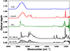 |
Fig. 3. Mid-IR spectra of pure EA and reference molecules NH3 and CH3OH at 10 K. The spectrum of H2O (common interstellar ice component) at 15 K is taken from the Leiden Ice Database for Astrochemistry (LIDA). Bands selected for band strength estimation are indicated by the shaded areas. |
IR band strengths for reference and molecules with functional group similar to EA.
where M is the molar mass, NA the Avogadro constant, and ρ the density of the molecule. ρNH3 = 0.68 g cm−3 was used for the calculation (Hudson et al. 2022), which ultimately yielded ANH3 = 22.3 × 10⁻¹⁸ cm mol−1.
To test how well this method works, we calculated the absolute band strength of NH3 using CH3OH as a reference and vice versa. In both cases, a set of two different Δp values were taken into consideration for each molecule. We obtained ANH3 = 26 ± 6 × 10⁻¹⁸ cm mol−1 in the former case, and in the latter, ACH3OH = 15 ± 3 × 10⁻¹⁸ cm mol−1. Within the errors, the deviation was around 10%. The estimated values of EA band strength for the three different integrated ranges by the two reference molecules are well within the errors, and they are summarized in Table 3. One standard deviation was used for the error calculation.
Estimated IR band strengths of EA ice at 10 K using three different methods.
The second method employed QMS measurements during TPD to obtain the column density of the molecules desorbed from the surface for band strength estimation. The species used were monitored through their primary mass fragment: m/z = 31 (CH3OH) and m/z = 30 (EA). It is worth mentioning that NH3 was excluded as a reference molecule in the second method due to the uncertainties associated with the relative transmission efficiency of the QMS between the m/z = 30 (EA) and m/z = 17 (NH3). This uncertainty can be neglected when using CH3OH as the reference molecule for Method 2 since the m/z ratios monitored are similar (m/z = 31 for CH3OH and m/z = 30 for EA). The integrated QMS signal measured during the TPD of a molecule is proportional to N and depends on several other parameters as highlighted by Maté et al. (2023). The band strength of EA in comparison to CH3OH can then be expressed as
 (4)
(4)
where I is the integrated QMS signal, σ the ionization cross-section for the first ionization of the species at 70 eV electron energy employed in the QMS, and f the fragmentation factor, which is the fraction of the primary fragment mass with respect to all the other fragment masses. The σ values for the two species are σCH3OH = 4.49 Å2 (Hudson et al. 2003) and σEA = 13.255 Å2 based on complex scattering potential-ionization contribution (CSP-ic) method (Chakraborty et al. 2024). The f values are fCH3OH = 0.404, and fEA = 0.648 (NIST database). The transmission efficiency can be considered equal. Considering all these correction parameters, the estimated EA band strength values deviated significantly from the values obtained by Method 1 as seen in Table 3. The possible cause for such deviation could be due to the uncertainty in the determination of different parameters used in Eq. (4).
The last method that we used (Method 3) consists of a series of temperature programmed desorption (TPD) measurements, which is a well-known technique in laboratory astrophysics (e.g. Burke & Brown 2010; Doronin et al. 2015). EA ices are grown at 100 K by exposing a KBr substrate to a partial pressure between 10−9 and 10−8 Torr of EA for a few minutes. Then the substrate is warmed up to 250 K using a ramp of 10 K min−1 and the thermal desorption of EA is probed as a function of the substrate temperature by following the m/z = 30 channel of the QMS. Figure 4 shows the TPD curves for different depositions of EA ices. According to the Polanyi-Wigner description of thermal desorption, we estimate the ML coverage of EA from these TPD curves. For multilayer depositions (red curves), the TPD curves display a common leading edge at the start of the desorption kinetics, from 165 K to 175 K, whereas for monolayer or sub-monolayer depositions (blue curves), this leading edge differs for each deposition. Based on those considerations and assuming that depositions are homogeneous and that the TPD integral is linear with the coverage, we estimate the EA coverage as shown in the legend of Fig. 4. IR measurements are also taken after each deposition before the onset of the TPD measurements. A good signal-to-noise ratio could only be obtained in the IR spectrum for coverages greater than 3.4 ML. Therefore, we used that in the determination of the IR band strength. Knowing the ice thickness associated with this IR spectrum, we therefore deduced the band strengths as displayed in Table 3 (Method 3). The evaluated band strength values show less deviation than Method 2. In Method 3, there could be uncertainties in the accurate determination of monolayer coverage, which could explain the deviation between Method 1 and Method 3. The error in Method 3 is computed from the relative difference obtained on the coverage of the 3.4 ML TPD curve when considering the actual 1.6 ML TPD curve to correspond to 1 ML. This results in a 38% uncertainty. Note that we have only used a few monolayer coverage equivalent of EA on the cold surface for band strength estimation by the three methods described above.
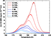 |
Fig. 4. Thermal desorption signal of EA from pure EA ices deposited at 100 K, and using a ramp of 10 K min−1. The coverage associated with each curve is based on the considerations as explained in the text. |
The advantage of Method 1 is the ease of band strength measurements of unknown molecules without the need for a dedicated experimental setup and the time for undertaking the experiment. This is especially suitable for larger organic molecules that are unstable and can undergo polymerization with time. The major advantage of Method 3 is that one can easily obtain the binding energy of the molecule of interest together with the band strength. On the other hand, the inconsistent variation of band strength estimation with Method 2 highlights the need for measuring parameters such as the ionization cross-section, the fragmentation factor, and the transmission efficiency of molecules in the laboratory through the QMS. Many researchers use an alternative approach, which involves laser interferometry. However, this method requires additional equipment and knowledge of the refractive index mass density of the ice formed. Furthermore, it assumes that the ice layer on the substrate is perfectly flat with zero porosity, which is not always the case. Therefore, this method can only be recommended when Method 1 cannot be applied, such as when measuring substances with low vapour pressures. Based on the discussion herein, we think that the three measurement approaches taken in this paper can all be used in the ways described in this work. From the comparison of the band strength values obtained from three methods, we think the direct method based on mass spectrometer and indirect method based on pressure gauge would provide a reliable determination of the band strengths.
Furthermore, alongside the three aforementioned methods, we have included absolute IR band strengths derived from theoretical calculations in Table 1. A satisfactory agreement exists between experimental and theoretical values for the NH2 bending mode at 1607 cm−1, considering the inherent approximations in both experimental and theoretical approaches. While this method may be effective for estimating individual vibration modes, it may not be suitable when considering combinations of various modes.
The observed double peak structure in the TPD could arise from two potential causes. Firstly, it may result from some degree of non-uniformity in film growth across the substrate during EA deposition using a 0.5 mm diameter capillary tube (Potapov et al. 2019). Secondly, the presence of minor hydroxyl group contamination on KBr could induce H-bonding interactions with EA, thereby contributing to the observed double peak structure. For multilayer desorption, with the coincident leading edge behaviour seen in the TPD trace, the desorption energy was then determined using an Arrhenius analysis of the leading edge region for the 3.4 ML curve as described previously in details (Suhasaria et al. 2015). The method yields the multilayer desorption energy of 0.61 ± 0.01 eV and the pre-exponential factor of 0.5 × 1027 molecule cm−2 s−1. In the literature, the binding energy of EA from carbon and water surface has been predicted via machine learning to be around 0.7 ± 0.2 eV (Villadsen et al. 2022). Although one cannot compare the values directly, the binding energy of EA from pure EA ice seems to be in good agreement with the predicted values within the errors. For systems with more complex desorption kinetics, transition state theory can be employed as a method to derive the pre-exponential factor (Thrower et al. 2013; Suhasaria et al. 2015).
4. Astrophysical implications
EA has been identified in both the interstellar medium and meteorites (Rivilla et al. 2021; Glavin et al. 2010), indicating its likely origin in space and its potential delivery to early Earth. This suggests a possible role for EA in the formation of crucial prebiotic molecules like amino acids, potentially contributing to the emergence of life (Rivilla et al. 2021). Furthermore, since EA can be formed via aminoketene, a link may exist between EA and peptides, which are also produced through aminoketene (Krasnokutski et al. 2022). Therefore, the detection of EA in both gas and solid phases across various sources such as molecular clouds and protoplanetary disks could indicate chemical processes essential for the origin of life. Accurately determining EA abundance or providing at least an upper limit in different conditions is therefore crucial for gaining reliable insights.
The gas-phase molecular column density of EA toward the G+0.693 molecular cloud in the SgrB2 complex in the Galactic centre was estimated at 1.5 × 1013 cm−2. This suggests an estimated abundance ranging from 0.9 to 1.4 × 10⁻¹⁰ relative to molecular hydrogen and the EA/H2O abundance ratio of the order of 10−6 (Rivilla et al. 2021). In the Almahata Sitta meteorite, the ratio EA/H2O was also found to be of the same order (Glavin et al. 2010). While ice signatures of EA have not been detected, it is reasonable to assume that the EA abundance is significantly higher in the solid state than the gas phase given the various solid-state pathways suggested on grains (Rivilla et al. 2021). In the gas phase, EA molecules might easily dissociate under UV photon irradiation due to their predominantly single bonds and relatively small size, making them more fragile and less capable of dissipating energy. Conversely, higher stability and potentially consequential reactions are expected for EA in the solid state.
The enhanced sensitivity of the Medium Resolution Spectrograph (MRS) (Wells et al. 2015) of the Mid-IR Instrument (MIRI) (Rieke et al. 2015; Wright et al. 2015) onboard the JWST compared to its predecessors raises the possibility of identifying solid EA in various astrophysical environments in the future. Figure 5 illustrates a comparison of the pure EA ice spectrum at 10 K with an observed JWST spectra of the low-mass protostar IRAS 2A taken with the MRS MIRI (Rocha et al. 2024). As can be seen from Fig. 5, the NH2 deformation mode of EA coincides with the strong features observed in the JWST spectra. However, many other molecules with NH2 and even C=C bands can contribute to the same feature. Figure 3 shows the spectrum of pure amorphous and crystalline EA ice along with the spectra of some of the common polar interstellar ice components. All of the EA ice features overlap with the common interstellar ices, and it could be challenging to significantly constrain the EA abundance. However, within environments where grain temperatures exceed the water desorption temperature (Td ∼ 160 K), the majority of volatile components within the ice mantle will sublimate. This process would result in an elevated concentration of EA (Td > 180 K) in the solid state. In this case, the band at 1607 cm−1 assigned to NH2 bending can be used to determine the column density of EA. Moreover, within astrophysical environments characterized by elevated temperatures (> 170 K), such as those found in protoplanetary disks, EA ice may manifest in a crystalline state. This crystalline form displays distinct sharp characteristics that distinguish it from other types of refractory ice. Finally, even at low temperatures (< 150 K) where volatile ice exists, it is possible to subtract the spectral features of known components such as NH3, CH3OH, H2O, and even silicates to detect EA. This process may result in a loss of sensitivity, but it will not prevent the detection or estimation of the upper limit of the abundance of EA.
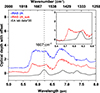 |
Fig. 5. Comparison of the JWST/MIRI MRS spectra of IRAS 2A (blue curve) and IRAS 2A with water:silicate features subtracted (red curve) to the laboratory-measured EA ice profile at 10 K. For clearer comparison, all spectra are vertically shifted, and the laboratory spectrum intensity is multiplied by 20, and the EA band at 1607 cm−1 is indicated by dashed line. The inset provides a closer examination of the water:silicate subtracted IRAS 2A spectrum alongside the fitted EA profile for upper limit estimation. |
In this work, we have estimated the upper limit of EA by comparing the laboratory data with the observed spectrum. The spectrum from IRAS 2A with water:silicate features subtracted was used to constrain the EA upper limit abundance. The EA feature at 1607 cm−1 (6.22 μm) marked with vertical dashed line was used for this purpose. The column density upper limit (N, in cm−2) of EA can be estimated using the following relation described in detail in Rachid et al. (2021):
 (5)
(5)
where, A = 1 × 10⁻¹⁷ cm molecule−1 is the band strength, and FWHM = 50.5 cm−1 for the 1607 cm−1 EA feature. τν is the maximum optical depth of the water:silicate subtracted peak where the EA peak centred at 1607 cm−1 fits. The inset to Fig. 5 shows the procedure for obtaining the maximum optical depth. Using this method, an upper limit of ≤4.4 × 1018 cm−2 was estimated, which corresponds to about 15% with respect to H2O, assuming a column density of 3 × 1019 cm−2 for water (Rocha et al. 2024). An abundance of EA this high seems improbable, and as previously noted, the 1607 cm−1 EA feature used for estimating abundance could also originate from other molecules. Apart from the upper limit estimation, the band strength estimation is also needed for the quantitative estimation of the photolysis products of EA. Improving the accuracy with which we know the initial concentration of the starting material will help us to better calculate the product yield.
In Table 2, we have listed the band strengths of the reference molecules (NH3 and CH3OH) used for band strength estimation of EA and of some other molecules that could potentially exist in interstellar medium and have one or both the functional groups (saturated and unsaturated) present in EA. Although one cannot directly compare the band strength values, a closer look indicates that the order of magnitude is similar to other molecules listed.
5. Conclusions
Solid EA was deposited on KBr substrate at 10 K, and IR spectra of the amorphous ice were measured. Band assignments were made by comparison with the calculated spectra. The EA ice was then annealed up to 250 K. Transmission spectra were recorded over the entire temperature range. Between 175 and 185 K, the amorphous EA phase undergoes a transition to the crystalline phase. IR band strengths were measured for amorphous EA ice. Three different methods were used to derive the band strengths. One of the three methods used a complete set of TPDs for EA from sub-ML coverage to the multilayer regime. The multilayer binding energy and the pre-exponential factor were determined experimentally. For gases whose pressure can be precisely measured in the gas line, the first tested method of determining absorption band strengths seems to be the simplest, giving satisfactory measurement accuracy, and can be recommended for use in laboratories. The second method requires precise knowledge of ion transport in the mass spectrometer, which is often missed, and the third method provides additional information but is relatively time-consuming and also involves uncertainties. A comparison between the laboratory data of pure EA and the JWST MIRI spectrum of the low-mass protostar IRAS 2A enabled us to derive an upper limit for the EA ice abundances with respect to solid H2O.
Acknowledgments
The authors are grateful to W.R.M. Rocha and E.F. van Dishoeck for providing the MIRI MRS JWST data. This work has been supported by the European Research Council under the Horizon 2020 Framework Program via the ERC Advanced Grant Origins 83 24 28. We would also like to acknowledge funding through the DeutscheForschungsgemeinschaft (DFG) project No. JA 2107/11-1. S.A.K. is grateful for the support from DFG (grant no. KR 3995/4-2). The authors also acknowledge support from the NanoSpace COST action (CA21126 – European Cooperation in Science and Technology).
References
- Bernstein, M. P., Dworkin, J. P., Sandford, S. A., Cooper, G. W., & Allamandola, L. J. 2002, Nature, 416, 401 [Google Scholar]
- Bouilloud, M., Fray, N., Bénilan, Y., et al. 2015, MNRAS, 451, 2145 [Google Scholar]
- Burke, D. J., & Brown, W. A. 2010, Phys. Chem. Chem. Phys., 12, 5947 [NASA ADS] [CrossRef] [Google Scholar]
- Canta, A., Öberg, K. I., & Rajappan, M. 2023, ApJ, 953, 81 [NASA ADS] [CrossRef] [Google Scholar]
- Chakraborty, I., Sinha, N., & Antony, B. 2024, Radiat. Phys. Chem., 216, 111421 [NASA ADS] [CrossRef] [Google Scholar]
- Doronin, M., Bertin, M., Michaut, X., Philippe, L., & Fillion, J.-H. 2015, J. Chem. Phys., 143, 084703 [NASA ADS] [CrossRef] [Google Scholar]
- Duvernay, F., Dufauret, V., Danger, G., et al. 2010, A&A, 523, A79 [NASA ADS] [CrossRef] [EDP Sciences] [Google Scholar]
- Frisch, M. J., Trucks, G. W., & Schlegel, H. B. 2016, Gaussian 16, Revision C.01 (Wallingford, CT: Gaussian Inc.) [Google Scholar]
- Gerakines, P. A., & Hudson, R. L. 2020, ApJ, 901, 52 [NASA ADS] [CrossRef] [Google Scholar]
- Glavin, D. P., Aubrey, A. D., Callahan, M. P., et al. 2010, Meteorit. Planet. Sci., 45, 1695 [NASA ADS] [CrossRef] [Google Scholar]
- González Díaz, C., Carrascosa, H., Muñoz Caro, G. M., Satorre, M. Á., & Chen, Y. 2022, MNRAS, 517, 5744 [CrossRef] [Google Scholar]
- Holtom, P. D., Bennett, C. J., Osamura, Y., Mason, N. J., & Kaiser, R. I. 2005, ApJ, 626, 940 [Google Scholar]
- Hudson, R. L. 2017, Spectrochim. Acta A, 187, 82 [NASA ADS] [CrossRef] [Google Scholar]
- Hudson, R., & Moore, M. 2004, Icarus, 172, 466 [Google Scholar]
- Hudson, J. E., Hamilton, M. L., Vallance, C., & Harland, P. W. 2003, Phys. Chem. Chem. Phys., 5, 3162 [Google Scholar]
- Hudson, R. L., Ferrante, R. F., & Moore, M. H. 2014, Icarus, 228, 276 [NASA ADS] [CrossRef] [Google Scholar]
- Hudson, R. L., Gerakines, P. A., & Yarnall, Y. Y. 2022, ApJ, 925, 156 [NASA ADS] [CrossRef] [Google Scholar]
- Krasnokutski, S. A. 2021, Low Temp. Phys., 47, 199 [NASA ADS] [CrossRef] [Google Scholar]
- Krasnokutski, S. A., Chuang, K. J., Jäger, C., Ueberschaar, N., & Henning, T. 2022, Nat. Astron., 6, 381 [NASA ADS] [CrossRef] [Google Scholar]
- Krasnokutski, S. A., Jäger, C., Henning, T., et al. 2024, Sci. Adv., 10, eadj7179 [NASA ADS] [CrossRef] [Google Scholar]
- Maté, B., Tanarro, I., Timón, V., Cernicharo, J., & Herrero, V. J. 2023, MNRAS, 523, 5887 [CrossRef] [Google Scholar]
- Molpeceres, G., Tsuge, M., Furuya, K., et al. 2024, J. Phys. Chem. A, 128, 3874 [NASA ADS] [CrossRef] [Google Scholar]
- Potapov, A., Jäger, C., & Henning, T. 2019, ApJ, 880, 12 [NASA ADS] [CrossRef] [Google Scholar]
- Rachid, M., Brunken, N., De Boe, D., et al. 2021, A&A, 653, A116 [NASA ADS] [CrossRef] [EDP Sciences] [Google Scholar]
- Räsänen, M., Aspiala, A., Homanen, L., & Murto, J. 1983, J. Mol. Struct., 96, 81 [CrossRef] [Google Scholar]
- Rieke, G. H., Wright, G., Böker, T., et al. 2015, PASP, 127, 584 [NASA ADS] [CrossRef] [Google Scholar]
- Rivilla, V. M., Jiménez-Serra, I., Martín-Pintado, J., et al. 2021, Proc. Natl. Acad. Sci., 118, e2101314118 [NASA ADS] [CrossRef] [Google Scholar]
- Rocha, W., van Dishoeck, E., Ressler, M., et al. 2024, A&A, 683, A124 [NASA ADS] [CrossRef] [EDP Sciences] [Google Scholar]
- Silva, C. F., Duarte, M. L. T., & Fausto, R. 1999, J. Mol. Struct., 482, 591 [CrossRef] [Google Scholar]
- Sladkova, A. A., Lisovskaya, A. G., Sosnovskaya, A. A., Edimecheva, I. P., & Shdyro, O. I. 2014, Radiat. Phys. Chem., 96, 229 [NASA ADS] [CrossRef] [Google Scholar]
- Suhasaria, T., Thrower, J., & Zacharias, H. 2015, MNRAS, 454, 3317 [NASA ADS] [CrossRef] [Google Scholar]
- Thrower, J. D., Friis, E. E., Skov, A. L., et al. 2013, J. Phys. Chem. C, 117, 13520 [NASA ADS] [CrossRef] [Google Scholar]
- Tseng, C.-L., Chen, Y.-K., Wang, S.-H., Peng, Z.-W., & Lin, J.-L. 2010, J. Phys. Chem. C, 114, 11835 [NASA ADS] [CrossRef] [Google Scholar]
- Villadsen, T., Ligterink, N. F., & Andersen, M. 2022, A&A, 666, A45 [NASA ADS] [CrossRef] [EDP Sciences] [Google Scholar]
- Vinogradoff, V., Duvernay, F., Danger, G., et al. 2013, A&A, 549, A40 [NASA ADS] [CrossRef] [EDP Sciences] [Google Scholar]
- Wells, M., Pel, J.-W., Glasse, A., et al. 2015, PASP, 127, 646 [NASA ADS] [CrossRef] [Google Scholar]
- Wright, G., Wright, D., Goodson, G., et al. 2015, PASP, 127, 595 [NASA ADS] [CrossRef] [Google Scholar]
All Tables
IR band strengths for reference and molecules with functional group similar to EA.
All Figures
|
Fig. 1. Experimental and theoretical mid-IR spectrum of EA. The upper one shows about 200 monolayers (ML) of EA condensed on KBr at 10 K. The IR bands marked with asterisks are due to a mixture of different vibrational modes. For the latter, calculations were performed at MP2/Aug-cc-pVTZ level. |
| In the text | |
|
Fig. 2. Series of mid-IR spectra of EA shown at different temperatures and two different spectral regions. About 200 ML of EA were initially condensed on the KBr surface at 10 K and warmed up to 250 K with a linear heating ramp. Spectra are shifted in ordinate for clarity. The spectrum at 190 K is made bold to indicate the complete phase transition from amorphous to crystalline. |
| In the text | |
|
Fig. 3. Mid-IR spectra of pure EA and reference molecules NH3 and CH3OH at 10 K. The spectrum of H2O (common interstellar ice component) at 15 K is taken from the Leiden Ice Database for Astrochemistry (LIDA). Bands selected for band strength estimation are indicated by the shaded areas. |
| In the text | |
|
Fig. 4. Thermal desorption signal of EA from pure EA ices deposited at 100 K, and using a ramp of 10 K min−1. The coverage associated with each curve is based on the considerations as explained in the text. |
| In the text | |
|
Fig. 5. Comparison of the JWST/MIRI MRS spectra of IRAS 2A (blue curve) and IRAS 2A with water:silicate features subtracted (red curve) to the laboratory-measured EA ice profile at 10 K. For clearer comparison, all spectra are vertically shifted, and the laboratory spectrum intensity is multiplied by 20, and the EA band at 1607 cm−1 is indicated by dashed line. The inset provides a closer examination of the water:silicate subtracted IRAS 2A spectrum alongside the fitted EA profile for upper limit estimation. |
| In the text | |
Current usage metrics show cumulative count of Article Views (full-text article views including HTML views, PDF and ePub downloads, according to the available data) and Abstracts Views on Vision4Press platform.
Data correspond to usage on the plateform after 2015. The current usage metrics is available 48-96 hours after online publication and is updated daily on week days.
Initial download of the metrics may take a while.