| Issue |
A&A
Volume 617, September 2018
|
|
|---|---|---|
| Article Number | A12 | |
| Number of page(s) | 16 | |
| Section | Planets and planetary systems | |
| DOI | https://doi.org/10.1051/0004-6361/201833023 | |
| Published online | 12 September 2018 | |
Taxonomic classification of asteroids based on MOVIS near-infrared colors★
1
Instituto de Astrofísica de Canarias (IAC), C/Vía Láctea s/n,
38205
La Laguna,
Tenerife,
Spain
2
Departamento de Astrofísica, Universidad de La Laguna,
38206
La Laguna,
Tenerife,
Spain
e-mail: This email address is being protected from spambots. You need JavaScript enabled to view it.
3
Astronomical Institute of the Romanian Academy,
5 Cuţitul de Argint,
040557
Bucharest,
Romania
4
Observatório Nacional,
rua Gal. José Cristino 77,
São Cristóvão,
20921-400
Rio de Janeiro,
Brazil
5
Department of Physics, University Politehnica of Bucharest,
Bucureşti
060042,
Romania
Received:
14
March
2018
Accepted:
14
June
2018
Abstract
Context. The MOVIS catalog contains the largest set of near-infrared (NIR) colors for solar system objects. These data were obtained from the observations performed by VISTA-VHS survey using the Y, J, H, and Ks filters. The taxonomic classification of objects in this catalog allows us to obtain large-scale distributions for the asteroidal population, to study faint objects, and to select targets for detailed spectral investigations.
Aims. We aim to provide a taxonomic classification for asteroids observed by VISTA-VHS survey. We derive a method for assigning a compositional type to an object based on its (Y − J), (J − Ks), and (H − Ks) colors.
Methods. We present a taxonomic classification for 18 265 asteroids from the MOVIS catalog, using a probabilistic method and the k-nearest neighbors algorithm. Because our taxonomy is based only on NIR colors, several classes from Bus-DeMeo were clustered into groups and a slightly different notation was used: i.e., the superscript indicates that the classification was obtained based on the NIR colors and the subscript indicates possible misidentifications with other types. Our results are compared with the information provided by the Sloan Digital Sky Survey (SDSS) and Wide-field Infrared Survey Explorer (WISE).
Results. The two algorithms used in this study give a taxonomic type for all objects having at least (Y − J) and (J − Ks) observed colors. A final classification is reported for a set of 6496 asteroids based on the criteria that kNN and probabilistic algorithms gave the same result, and the color errors are within the limits (Y − J)err ≤ 0.118 and (J − Ks)err ≤ 0.136. This set includes 144 bodies classified as Bkni, 613 as Cni, 197 as Cgxni, 91 as Xtni, 440 as Dsni, 665 as Klni, 233 as Adni, 3315 as Sni, and 798 as Vni. We report the albedo distribution for each taxonomic group and we compute new median values for the main types. We found that V-type and A-type candidates have identical size frequency distributions, but V types are five times more common than A types. Several particular cases, such as the A-type asteroid (11616) 1996 BQ2 and the S-type (3675) Kematsch, both in the Cybele population, are discussed.
Key words: minor planets, asteroids: general / techniques: photometric / techniques: spectroscopic / methods: observational / methods: statistical
Classification table for 18 265 asteroids is only available at the CDS via anonymous ftp to cdsarc.u-strasbg.fr (130.79.128.5) or via http://cdsarc.u-strasbg.fr/viz-bin/qcat?J/A+A/617/A12
© ESO 2018
1 Introduction
Spectrophotometric data in the near-infrared (NIR) region have been used for a long time to characterize the surface composition of asteroids (e.g., Johnson et al. 1975; Veeder et al. 1982; Hahn & Lagerkvist 1988; Sykes et al. 2000; Mommert et al. 2016). Comparative planetology, which is the interpretation of reflectance spectra by direct comparison with laboratory data, was one of the first tools used to analyze telescopic observations (e.g., Johnson et al. 1975).
Early works (e.g., Veeder et al. 1982) showed that carbonaceous and silicate-like compositions can be determined based on J, H, and Ks observations. As more data became available, evidence of several compositional groups appeared. These were represented by various taxonomic classes that occupy well-defined regions in the NIR color–color plots (Hahn & Lagerkvist 1988). Thus, spectrophotometry in the NIR region proved to be a method of obtaining compositional information for faint targets that are not available for spectroscopic studies. It has been recognized as one of the best current techniques for surveying a large number of distant populations such as Centaurs and trans-Neptunian objects (e.g., Perna et al. 2010).
The goal of asteroid taxonomy (a term derived from the ancient Greek words taxis, i.e., arrangement, and nomia, i.e., method) is to identify groups of objects that have similar compositions. The classification schema is defined by statistically processing spectrophotometric, spectral, and polarimetric data of a significant number of objects.
The first defined taxons (i.e, a taxonomic category) of asteroids were denominated by letters according to the compositional interpretation inferred from the observations in the visible wavelengths: C refers to carbonaceous, asteroids with observed properties similar to carbonaceous chondrite meteorites, and S refers to stony, asteroids that showed the distinct signature (i.e., 1 μm band) of pyroxene or olivine mixtures (Chapman et al. 1975). Chapman et al. (1975) noticed that more than 90% of their observed minor planets fell into these two broad groups. This way of denominating groups continued as new data were reported. For example, E stands for compositions such as enstatite meteorites, M for metallic asteroids, and R for the objects with the reddest colors and moderately high albedos (Bowell et al. 1978).
The increasing amount of spectral data over the visible and NIR wavelength region increased the number of taxons by taking into account subtle features. Two of the latest and widely used taxonomies are Bus & Binzel (2002a), who defined 26 classes using data over the 0.44–0.92 μm spectral interval, and DeMeo et al. (2009), who defined 24 classes based on data over the 0.45–2.45 μm wavelength range. The main groups initially defined translated into broad complexes (S complex, C complex, and X complex) followed by end-member types (A, D, K, L, O, Q, R, and V). Carvano et al. (2010) noted the fact that spectra similar to the templates proposed by the taxonomic systems were systematically recovered by independent authors using diverse datasets and different observing techniques, providing confidence in these systems.
However, the classification accuracy in a taxonomic scheme depends on the observational data available. If only a part of the data is measured (i.e., spectrum over a short spectral interval or just spectrophotometric data), it is still possible to assign a type, but the level of confidence decreases. Various methods can be applied. These methods range from directly forging the observational data into the schema to different parameterizations and transformations (e.g., principal component analysis) of the observed values. The problem of classifying new data can be summarized as defining the parameters to be used, mapping the regions corresponding to different groups, and selecting a definition for the distance in this space.
The sky surveys provide a large amount of data for solar system objects (e.g., Sykes et al. 2000; Baudrand et al. 2001; Ivezić et al. 2001; Carry et al. 2016). But, except for the spectroscopic surveys of asteroids (e.g., Xu et al. 1995; Bus & Binzel 2002b; Lazzaro et al. 2004) that observed several thousands of objects, large observational datasets are limited to broadband photometric filters. In this case a classification using an extended schema such as DeMeo et al. (2009) is not possible. In order to retrieve the compositional information, several versions of taxonomies corresponding to broad classes were developed (e.g., Sykes et al. 2000; Misra & Bus 2008; Carvano et al. 2010; DeMeo & Carry 2013; Roh et al. 2016) in close relation with well-known taxonomies (Tholen 1984; Bus & Binzel 2002a; DeMeo et al. 2009). One method of linking the colors with the spectral behavior for the SDSS data, which is the survey that provided the largest amount of data for solar system objects in the visible region, was to define the locus of each class in the parameter space using observations of previously classified asteroids (typically from SMASS and S3OS2 survey), meteorite spectra, and synthetic spectra (Carvano et al. 2010).
Taxonomic classification provides rough information about the surface composition of an asteroid. Accurate mineralogical characterization requires high quality spectra. However, from an observational point of view, assigning an object to a class based on spectrophotometric data has several advantages compared to spectral studies; it requires less observing time, the faint targets (i.e., small objects or those at large heliocentric distances) can be characterized, and big datasets are available from the sky surveys (DeMeo & Carry 2014).
The aim of our work is to classify the asteroids based on the NIR colors provided by the MOVIS-C catalog (Popescu et al. 2016) using a schema fully compatible with the taxonomy defined by DeMeo et al. (2009). This study also proposes methods to investigate future survey data such as the spectrophotometric observations of the solar system objects, which will be observed by the Euclid survey (Laureijs et al. 2011; Carry 2018).
The MOVIS-C catalog was built based on VISTA-VHS survey and provides the largest set of NIR data up to now. Theobservations included three programs: (1) the VHS-GPS (Galactic Plane Survey), which uses J and Ks filters; (2) the VHS-DAS (Dark Energy Survey), which uses J, H, and Ks filters; and (3) the VHS-ATLAS, which uses Y, J, H, and Ks filters (Irwin et al. 2004; Lewis et al. 2010; Cross et al. 2012; McMahon et al. 2013; Sutherland et al. 2015). The number of measured colors for each solar system object varies according to the observing strategy and to the limiting magnitude of each filter. Also depending on the survey plan, the observations that enter in the computation of a color are distanced by different time intervals. The colors that are less affected are (Y − J), (J − Ks), and (H − Ks) for which the time span between two observations is about 7 min (see Popescu et al. 2016; Morate et al. 2018, for a complete description). These colors were selected for assigning a taxonomic class.
This paper is organized as follows. Section 1 presents the data preparation and the framework for the classification schema. The methods used for the classification are described in Sect. 3. The results are summarized in Sect. 4 and discussed with respect to WISE albedo and SDSS data. Several implications of our findings are shown in Sect. 5. A review of future perspectives is made in Sect. 6 and conclusions are presented in Sect. 7.
2 Data preparation
2.1 Connecting spectra to NIR colors
The first step for inferring the compositional information from MOVIS-C NIR colors is to compute their relation with the spectral data. It was shown in the previous work (Popescu et al. 2016) that clear patterns appear in color–color plots of minor planets observed with the Y, J, H, Ks VISTA filters. The corresponding clusters can be linked to the taxonomic types defined by DeMeo et al. (2009).
The reflectance spectra of asteroids are obtained by dividing the observed spectral data of a minor planet by a G2V solar analog spectrum measured in similar conditions. The resulting curve is normalized (typically unity at 1.25 μm) because the shape of the features provides information about the surface composition. This technique is used for the V-NIR spectra for which the flux of the reflected light is much larger compared to the emitted thermal radiation (e.g., Popescu 2012). Thus, the transformation of the reflectance spectra into colors and vice versa requires that the spectrophotometric data of G2V stars are taken into account.
Synthetic colors can be computed from reflectance spectra in the following manner: (a) computing the flux (Ff) corresponding to a filter f by multiplying the spectrum of asteroid (Saster) by the transmittance curve of the filter, Hf (λ), and by the spectrum of a standard G2V star (SSun), and integrating the result with respect to wavelength (λ); and (b) obtaining the corresponding colors (Cf1−f2, where f1 and f2 are two different filters) by subtracting the magnitudes determined from the computed fluxes; this step involves a calibration constant, Ccalib, according to the magnitude system. These steps are described by Eqs. (1) and (2) as follows:
 (1)
(1)
 (2)
(2)
By considering the reflectance flux Rf = ∫ Hf ⋅ Raster dλ, the following approximation can be made: Eq. (3), where  is the color of the Sun corresponding to the filters f1 and f2. This introduces an error smaller than ~0.007 magnitudes (statistically computed by taking into account a large number of spectra). This error can be neglected when compared to typical errors from the MOVIS-C catalog, i.e.,
![Mathematical equation: \begin{equation*} C_{f1-f2} = -2.5[\textrm{log}_{10}R_{f1} - \textrm{log}_{10}R_{f2}] + C_{f1-f2}^{\textrm{Sun}}.\end{equation*}](/articles/aa/full_html/2018/09/aa33023-18/aa33023-18-eq10.png) (3)
(3)
The advantage of this approximation is to consider the colors of the Sun that can be measured from the G2V solar analogs in the same conditions as the colors obtained for the asteroid data.
Casagrande et al. (2012) provided the colors of the solar analogs based on the Two Microns All Sky Survey (2MASS). We searched the VISTA observations for G2V stars identified based on 2MASS. After having removed the outliers (i.e., colors outside 3σ interval from the median values), we took the medians and found the following values:  ,
,  ,
,  , and
, and  . The comparison with the values reported by Casagrande et al. (2012) and transformed to VISTA filter system (see Popescu et al. 2016 for the computation) shows the largest difference for the (Y − J) color (about 0.013). This can be attributed to the fact that the 2MASS survey did not use the Y filter and its value is extrapolated from the other three filters. Thus, the colors of G2V solar analogs used in this article are
  , resulting from current determination, and
  ,
,  ,
,  , resulting from Casagrande et al. (2012) after applying the transformation to VISTA filters.
Equation (3) can be reverted to obtain reflectances from colors, i.e.,
 (4)
(4)
In this case, the normalization can be made relative to the J filter ( ), which is consistent with spectral data. This relation is useful for describing the spectral parameters (e.g., slopes) based on the MOVIS-C colors and for comparing these parameters with existing data in the literature.
2.2 Reference colors
The taxonomic system defined by DeMeo et al. (2009) is one of the most commonly used for classifying asteroids using their reflectance spectra in the visible and NIR wavelength regions. The authors define 24 classes that closely follow the visible wavelength taxonomy of Bus & Binzel (2002a) and that of Tholen (1984). The taxons were obtained by applying principal component analysis (PCA) to a set of 371 spectra of asteroids for which the slope had been removed. The boundaries between classes were determined in the PC1–PC5 space. The reflectance values of the standard spectral types are defined for 41 wavelengths, equally distanced at 0.05 μm, over the 0.45–2.45 μm interval.
In order to obtain a classification that is compatible with that of DeMeo et al. (2009), the same spectral set has to be used as reference. Thus, we applied the transformation shown by Eq. (3) to the 371 spectra used to define the DeMeo et al. (2009) taxonomic system. For each class we obtained the mean value and standard deviation of (Y − J), (J − Ks), and (H − Ks) colors. These are summarized in Table A.1. All standard deviations smaller than 0.02 were limited to this value to account for other type of errors (e.g., approximations made by color computation, light curve variations, and solar color errors). The reflectance in the Y, J, H, and Ks filters for each standard spectral curve are shown in Fig. A.1.
We note that some of the classes in the DeMeo et al. (2009) taxonomy are defined based on a very low number of objects. This is the case for the A types (6 objects), B types (4 objects), Sa types (2 objects), Sv types (2 objects), and even Cg, O, and R types defined with a single object. Because of this, their limits are poorly constrained and the standard deviations are too large (A types), too small (Sa, Sv types), or undefined (for those classes represented by a single object). This uncertainty translates in the color domain, i.e., the color intervals covered by these types are insufficiently defined.
The ability of the VISTA filter set to distinguish between taxonomic classes can be assessed by looking at the distribution of the colors in each class. To illustrate the information contained by the (Y − J), (J − Ks), and (H − Ks) colors, we plot the average values and the standard deviation obtained for each color and spectral class (Fig. A.2). These plots show that the end-member A, B, and V types can be inferred by a single color. For example, the (Y − J) color allows the following assumptions: (1) because of the steepness of 1 μm band, an object with (Y − J) > 0.45 is an A type, an O type, an R type, or a V type; (2) the V types, within 2 , where
  is the standard deviation of V-type template, have (Y − J) ≥ ~0.5; 3) in general, the S complex has larger values of (Y − J) than the C complex, and there is a relative border between them at ~0.3; and (4) the B types have negative NIR slopes and they occupy the region with (Y − J) ≤ 0.219, which is the (Y −J) color of the Sun. A value of (J − Ks) > 0.8 indicates an extremely red NIR spectrum corresponding to A or D types.
The (Y − J) vs. (J − Ks) contains most of the information for separating the main taxonomic groups (Popescu et al. 2016). This result is emphasized by plotting the computed colors for the reference set (Fig. 1). Several remarks can be made. First, the region (Y − J) ≥ 0.5 and (J − Ks) ≤ 0.3 is distinctive (Licandro et al. 2017) and was identified as corresponding to V-type asteroids. Second, O and R types, whose spectra show a deep 1 μm absorption band and a shallow 2 μm feature, are in the interval (Y − J) ≥ 0.5 and 0.7 ≥ (J − Ks) ≥ 0.3. Third, the S complex can be separated from the C complex and the D type based on the line α(Y −J) = 0.412±0.046 × (J − Ks) + 0.155±0.016 (Popescu et al. 2016). This line marks the separation between the groups associated with silicaceous and carbonaceous compositions, but it cuts the K, L type regions that span intermediate color values. Using the (Y − J) value, we can further divide the area below the α line as follows: Dtypes have (Y − J) ≥ 0.3, B types have (Y − J) ≤ 0.219 and (J − Ks) ≤ 0.34, while C andX complexes are located between these two borders.
This description is an indication based on the computed colors of the reference spectral set. The real data deals with photometric errors, phase angle effects or reddening due to space weather, and light-curve variations that can change the categorization. To overcome this fact, we clustered the 24 classes defined by DeMeo et al. (2009) into several groups by considering similar compositional types and their distance in the {(Y − J), (J − Ks), (H − Ks)} parameter space. These groups are considered for classifying the observational data provided by the MOVIS-C catalog. They are described below by showing the analogous Bus-DeMeo types. The superscript index of each letter indicates that the group was defined based on NIR colors (ni) and the subscript indicates some possible confusions (the level of accuracy is discussed in the following sections).
-
 = (B) is characterized by NIR color values that are lower than those of the Sun. It is distinctive from the C-complex objects. A result found after studying the classified sample was that the close borders with the K types may give some confusion with this type; i.e., there are K types with blue NIR colors.
 -
Cni = (C, Cb) has higher (J − Ks) and (H − Ks) values compared to Cg,Cgh,Ch (Table A.1). This allows us to split the C complex into two groups. However, the distance between these groups in the color space is small (less than 0.1 mag.) and for the separation to be effective it requires accurate photometry. As it shown in Sect. 4 this group identifies with high probability (≥85%) to the low albedo asteroids.
-
 =(Cg,Cgh,Ch,Xc,Xe) covers multiple types from Bus- DeMeo taxonomy because the NIR colors are unable to separate some classes of the C complex from those of the X complex; thus, this group includes both low and high albedo asteroids. The colors corresponding to this group occupy an intermediate region between
Cni
and
=(Cg,Cgh,Ch,Xc,Xe) covers multiple types from Bus- DeMeo taxonomy because the NIR colors are unable to separate some classes of the C complex from those of the X complex; thus, this group includes both low and high albedo asteroids. The colors corresponding to this group occupy an intermediate region between
Cni
and  .
. -
 = (T, X, Xk) corresponds to objects with the highest color values from the X complex. It also includes both low and high albedo asteroids.
 -
 = (D) has the largest spectral slope in the NIR, compared to
  . The definition of DeMeo et al. (2009) is based on the V-NIR spectral data of 16 objects and it covers broad reflectance values. The reddest objects belonging to this group can be confused with the A, Sa types, and marginally with Sr.
 -
 , where the K and L types have intermediate color values between C and S complexes in the NIR color space. Based only on (Y − J), (J − Ks), and (H − Ks), the asteroids classified in this group can be misidentified with some of the S types or C types. The group also serves to reduce the misidentifications between the silicaceous and carbonaceous compositions associated with the C and S complexes.
 -
 = (A,Sa)is characterized by the reddest (J − Ks) color, a moderate to high (Y − J) color, and a moderate (H − K). The borders of the group are insufficiently determined in the color space (e.g., large σ(J−Ks) = 0.152 value) because of the low number of reference objects used for the definition of these classes (six for A and two for Sa) and because they are widely spread in the color space. The asteroids assigned to thisgroup based on MOVIS-C must have an extremely red NIR spectrum. A separation between
 and D types can be made by including the albedo value. This was unexpected from the investigation of the reference set, which does not include D types with such red values.
 -
Sni = (Q, S, Sq, Sv, Sr) corresponds to silicate-like compositions, which show spectral bands at 1 and 2 μm.
-
Vni = (V) is distinctive in the (Y − J) vs. (J − Ks) color–color space (Licandro et al. 2017). It corresponds to compositions similar to howardite-eucrite-diogenite meteorites (HED).
We note that the O and R types were not considered, as they are defined based on a single object. It is shown in the discussion section that there are several tens of objects with similar color values as these types. The L type is included in the same group as K type.
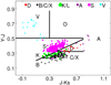 |
Fig. 1 (Y − J) vs. (J − Ks) color–color plot derived from the 371 spectra used to define the DeMeo et al. (2009) taxonomy. The main taxonomic types are plotted with different colors for comparison. A types include A and Sa types; C and X refer to C and X complexes; S types include the S complex and Q types. We indicate the limits for each taxonomic class assumed in this work with straight lines. |
2.3 MOVIS-C data selection and ranking
The VHSv20161007 data release contains 141132 logs of stack-frames corresponding to the observations acquired between November 4, 2009 and March 27, 2016. We obtained an updated version of MOVIS-C catalog containing the NIR colors for 53 447 solar system objects by running the pipeline described in Popescu et al. (2016) for this set of VISTA-VHS observations. The search was performed considering the objects listed in the ASTORB version of March 2017. We recovered color information for 57 NEAs (near-Earth asteroids), 431 Mars Crossers, 612 Hungaria asteroids, 51 382 main-belt asteroids, 218 Cybele asteroids, 267 Hilda asteroids, 434 Trojans, and 29 Kuiper Belt objects.
The details regarding the survey and the pipeline used to retrieve the colors from the observations catalogued by VISTA Science Archive, which is part of VISTA Data Flow System (Emerson et al. 2004; Hambly et al. 2004; Irwin et al. 2004; Lewis et al. 2010), are described by Popescu et al. (2016) and the references herein. We provide a brief summary. The magnitudes and fluxes were retrieved from the vhsDetection database1, which contains the sources from each individual stack frame. This type of image is obtained by adding typically two exposures of 7 or 15 sec each (depending on the program). The derived colors are the differences of the average magnitudes in each filter after the outliers and spurious data have been removed; typically there were at least two detections for each band.
The MOVIS-C colors catalog contains photometric observations with errors varying from accurate measurements (i.e., photometric errors less than 0.01 magnitude) up to the detection limit of the pipeline (i.e., about ≈0.4 magnitude error). A first approach to account for the uncertainties is to split the MOVIS-C catalog in four subsets using the quartiles defined on the distributions of the color magnitude errors for the (Y − J), (J − Ks), and (H − Ks). The quartiles aregiven by the thresholds that divide the dataset into four equal-size groups with respect to error. For example, the second quartile cutoff value corresponds to the median of errors. The subsets are denoted by Q1 (lower quartile), Q2 (median), and Q3 (upper quartile). Table 1 gives the upper error limits and the number of objects. The subsets are defined considering objects with measurements in three or four filters and with errors for the colors lower than the thresholds of the quartiles.
There are 37 634 objects with determined (Y − J) color, 31 750 with (J − Ks), and 11 268 with (H − Ks). The (Y − J) and (J − Ks) color space contains most of the information with respect to taxonomic type. There are 18 265 asteroids having both (Y − J) and (J − Ks) measured. In the best case when an object was observed with all four filters, we chose the (Y − J), (J − Ks), and (H − Ks) colors for the classification because they were obtained in similar time intervals of about ~7 min (Popescu et al. 2016).
In order to evaluate the possible errors introduced by the light curve variation we used the data available in the Asteroid Lightcurve Database2. The median rotation period for more than 18 000 asteroids is ~6.3 h, and the median of the light curve amplitudes is ~0.38 magnitudes. Statistically, these values translate into an uncertainty of ~0.03 magnitudes for (Y − J) and (J − Ks), which have about a ~7 min time interval between the observations with each filter.
Characteristics of the selected sample.
3 Methodology
The classification of asteroids based on colors is sensitive to magnitude uncertainties. The fact that the spectral interval is sampled by few broadband filters makes the uncertainties substantially account for the shape of the equivalent spectrum. In this context we used two approaches for classifying MOVIS-C data: a probabilistic approach following a similar schema to Carvano et al. (2010), which was successfully applied for SDSS data, and a second based on machine-learning algorithms provided with the scikit-learn3 module for Python (Pedregosa et al. 2011; Buitinck et al. 2013). The results reported using both methods are provided in the catalog accompanying the paper.
For implementing the probabilistic approach, we considered a normal distribution for each taxonomic type defined by DeMeo et al. (2009) in the {(Y − J), (J − Ks), (H − Ks)} color space. The distributions are defined based on the mean and standard deviation of colors (Table A.1) computed from the 371 spectra used for the definition of Bus-DeMeo taxonomy. The computation is performed as explained in Sect. 2.2. The normal distribution is widely used in the description of the natural phenomena. In this case there is no physical evidence supporting a particular type of distribution. This choice is made in a convenient way as it does not require us to define borders in the parameter space and outlines the continuity of the spectral features shown in the color–color plots. This continuity of spectral features was also observed with the visible colors provided by the SDSS data (Hasselmann et al. 2015).
For each observed color, we attributed a normal distribution around the nominal value with a standard deviation equal to the uncertainty of the measurement. The probability of the asteroid color of falling into the limits of a given class is calculated as the area of the distribution that overlaps the class distribution; the class is modeled as a Gaussian distribution with mean and standard deviation shown in Table A.1. The probability of the observation belonging to a taxonomic type is the product of the probabilities of all colors. This method provides a measure of how much aset of observations resembles a given template, which in this case is one of the 24 types defined by the Bus-DeMeo taxonomy. The class with the highest probability points to the taxonomic group assigned to the object.
A second approach for the classification schema is to use different machine-learning methods. A similar approach has been used by Mommert et al. (2016) for classifying near-Earth objects observed with Z, J, H, and K filters. For our analysis, we used the computed colors of the spectra presented by DeMeo et al. (2009) as the training set. The following methods were tested: Extreme Gradient Boosting (XGB), Random Forests (RF) with different parameters, and Nearest Neighbors (kNN).
To validate the algorithms we performed the so-called leave-one-out cross-test with respect to the training set. The test involves using one object from the reference set for validation and the remaining data as the training set. This is repeated for all objects in the training set. Table 2 compares the accuracy of classifications for these algorithms, considering two different cases: the first case assumes three-color observations {(Y − J), (J − Ks), (H − Ks)} and the second case assumes two-color measurements {(Y − J), (J − Ks)}. The accuracy results are comparable in the limit of 2%. Similar results were obtained by Mommert et al. (2016) using (Z − J), (J − H), and (J − Ks) colors based on a training sample of 319 synthesized asteroid colors.
We report the result of classification using the kNN (k = 3, 3NN) algorithm. Although 5NN performs slightly better than 3NN according to the leave-one-out test because for end-member classes we have a very small number of training samples (A-6 objects, B-4 objects, and D-16 objects), we decided to use the last one. This simple and effective method works well for identifying peculiar types. To account for the magnitude errors, we used a Monte Carlo approach: each measurement was randomized 106 times considering a Gaussian distribution with the color as the mean value and color error as the standard deviation. We counted the frequency ofclassification for each group to obtain the classification probabilities and we adopted the most likely taxonomic class for the target.
The confusion matrix (i.e., a matrix layout that allows the visualization of the performance of the algorithm) obtained after leave-one-out cross-test is shown in Fig. 2 for both algorithms. This approach shows a high accuracy for the large groups (S complex and C complex). The accuracy for the end-member groups Bni and  , which are defined based on a very low number of objects, must be taken with caution. One of the most significant interferences shown by the graph is between the
  and
and  types: both of these represent very red spectra and their NIR colors may coincide.
In general, the three-color case derives more accurate results based on the fact that the increased number of degrees of freedom puts additional constraints on the classification problem. The difference between the three-color case and two-color case is on the order of few percents, and it shows that the most relevant information is contained by the (Y − J) and (J − Ks) colors.
Both algorithms report a classification for each of the 18 265 asteroids that have the (Y − J) and (J − Ks) colors measured. The color errors are directly reflected into the probabilities of each class. If an object has an error bar that spans multiple classes it will have similar low probabilities for each of them. Moreover, for the objects that have large color errors and color values at the border of various classes it is likely that the two methods provide different results, which prevents us from reaching a conclusion regarding a classification.
We recall that individual objects follow the statistics shown in (Fig. 2) and their classification is made with a probability that depends on their color errors. The tables accompanying the paper provide the information for each object: the colors (including the colors errors and the time interval in which they were obtained), the classification results with the corresponding probabilities for each method, and the final classification.
Comparison between different classification algorithms based on the leave-one-out test performed with the computed colors from the spectra used for the definition of Bus-DeMeo taxonomy.
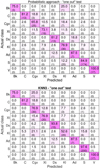 |
Fig. 2 Confusion matrix for the algorithms obtained after the leave-one-out cross-validation. It shows the classes predicted by the algorithm based on their computed colors vs. the spectral classification (labeled actual class) for the 371 samples of the reference set. The top panel shows the results for the probabilistic approach and the bottom panel shows the results for the k = 3 nearest neighbors (kNN3) algorithm. Each row of the matrix represents the instances (in terms of percentages computed relative to the total number of objects for the given spectral class) in the actual spectral class, while each column represents the instances in the class predicted by the algorithm (the number of instances is given within the parenthesis). The color intensity outlines the interferences. |
4 Results
We assigned a final taxonomic type based on kNN and probabilistic algorithms. This assignment was made when both methods gave the same result and the color errors are within the Q2 limits, i.e., (Y − J)err ≤ 0.118 and (J − Ks)err ≤ 0.136. This is the case for 6496 objects. All others that fail these conditions are marked with the letter U (undefined); these are asteroids forwhich a final classification cannot be made based on our dataset. In order to assign a final taxonomic classification, we did not constrained the probabilities to be higher than a certain threshold. However, we note that 75% (and 90% when considering only the 3NN probabilities) objects with a final taxon have both probabilities larger than 0.5 and the statistical results reported below are not sensitive to this selection.
The setof 6496 solar system bodies for which a final class was assigned includes 144  , 613 Cni, 197
  , 91
, 91  , 440
, 440  , 665
, 665  , 233
, 233  , 3315 Sni, and 798 Vni. These numbers are strongly dependent on the observational biases (high albedo objects are brighter and thus are more likely to be observed than the low albedo objects) and on the classification method (objects with prominent spectral features, i.e., V types, are easily identified compared to those that show small NIR color variations between different types).
We do not assign a taxonomic type for about one-third of the Q2 samples because the results provided by the two algorithms (probabilistic and kNN3) are different. Some of the cases belong to color space domains where different groups overlap. Other unclassified asteroids may have compositions unaccounted by taxonomy, a point that is addressed in the discussion section using the (Y − J) vs. (J − Ks) color plot.
A sample of the asteroids reported in MOVIS-C catalog is classified using SDSS data (Carvano et al. 2010), and has the visual albedo (pV) determined based on WISE observations (Masiero et al. 2011; Mainzer et al. 2011a, 2014). Our results are discussed in the context of the information provided by these two large surveys. We used the Minor Planet Physical Properties Catalogue4 (MP3C) and the Small Bodies Node of the NASA Planetary Data System5 (PDS) to retrieve the corresponding information.
The MOVIS-C catalog contains information for 6299 asteroids belonging to collisional families (Nesvorný et al. 2015). We report a final taxonomic classification for 1874 (about 28.8% from the classified objects) of these and we show how many asteroids of each class are assigned to families. An in-depth study of NIR colors of asteroid families is provided by Morate et al. (2018).
4.1 Comparison with the SDSS dataset
In the sample of asteroids classified based on MOVIS-C NIR data, there are 1467 objects for which a taxonomic type was reported by Carvano et al. (2010) using SDSS visible colors. This gives us the opportunity to study the variation of colors over the visible to NIR interval for a large dataset.
Following the definitions of the taxonomic types from this paper and those from Carvano et al. (2010), we computed the cross-tabulation matrix for the two classifications (Fig. 3). At first glance this shows the matching between the two results. Furthermore, this cross matrix also underlines spectrophotometric behavior not accounted by the current taxonomies.
There is a significant matching between the two sets of data for identifying carbonaceous (i.e., objects characterized by featureless spectra) and olivine-pyroxene (i.e., objects characterized by bands at 1 and 2 μm) compositions. The main sections of the cross-tabulation matrix correspond to ( , Cni,
  ,
,  )MOVIS vs. (C, X)SDSS (top left), and (Sni, Vni)MOVIS vs. (S/Q, V)SDSS (bottom right). These sections outline the main compositional types.
About 68.1% (143 asteroids) from the objects classified as  , Cni,
  correspond to CSDSS group, while a fraction of 16.7% of the objects are found as XSDSS. Concerning the silicate-like compositions, there are 552 objects belonging to S complex according to both datasets (78.4% matching). Some of the Sni asteroids are reportedas LSDSS type (13.6%, 96 asteroids).
Although the leave-one-out test gives a probability higher than 80% for classifying the  types, there is a significant difference when comparing them with their classification based on SDSS data (Fig. 3). An explanation for the 29 objects reported as
  and as SSDSS are the asteroids with high content of olivine, which show a red spectrum and a weak 2 μm band, such as those classified as Sa (Fig. A.1) by DeMeo et al. (2009). Also S-type objects with high NIR spectral slopes (marked with “w” in Bus-DeMeo taxonomy) may account for an explanation for the mismatch. The albedo values provided by the WISE survey confirm the silicate nature of this sample.
Only 25 objects are found as  – LSDSS. Most of the
  asteroids were classified by Carvano et al. (2010) as CSDSS types (66 objects, 42.3%) or SSDSS types (28 objects, 17.9%). This is because K and L types (as were defined by Bus-DeMeo taxonomy) do not show a prominent spectral features typical of the S types in the NIR, but they are not featureless either, like C types.
There are only three olivine rich asteroids (described by  group) identified by both surveys. About 19 objects classified as
  are found as SSDSS type. The NIR colors suggest for this sample an olivine rich composition or may indicate a reddening due to space-weathering effect. A noticeable interference consists of the 15 asteroids (29.4%) found as
  and that were reported as DSDSS. This crosstalk is also seen on the leave-one-out test (Fig. 2). Because of the reference set, which does not have D types with high NIR spectral slope, all MOVIS-C data with extremely red NIR colors are reported as
  . In this case albedos, or SDSS colors, provide a way to discriminate between the D and A types from Bus-DeMeo taxonomy.
A particular case is that of 24 asteroids with SDSS C-type colors and found as  or
or  . This suggests a spectral behavior neutral or slightly red in the visible, which turns red to extremely red in the NIR wavelengths. A similar behavior has been previously reported by de León et al. (2012), showing that asteroids classified as B types from their visible spectra presented a variety of shapes in the NIR, from blue to moderately red spectral slopes.
We notethat spectral studies have to confirm the characterization of individual objects because the color errors reported by both surveys can significantly change the conclusion. Figure 3 provides a statistical view of the cross-matching between the two large datasets. The relevance of the percentages has to consider the number of instances (i.e., the number of objects reported for each element of the matrix).
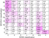 |
Fig. 3 Cross-tabulation matrix between the classification obtained based on MOVIS-C data (this work) and that obtained from SDSS data (Carvano et al. 2010). The percentages are specified relative to MOVIS-C assigned type, and the number of objects is specified within parenthesis. The color intensity outlines the interferences. |
4.2 Extremely red colors:  and
and 
The asteroids classified as  have (J − Ks) ≳ 0.65 and the average value (J − Ks)avg = 0.84 ± 0.17. This is the only group with such a red color (see Fig. 1 and Table A.1). The distribution of their albedo, available from the WISE measurements for 117 of these objects, spans large intervals covering both silicaceous and carbonaceous compositions (Fig. 4).
A-type asteroids (e.g., Veeder et al. 1983; Bus & Binzel 2002a; DeMeo et al. 2009) are associated with olivine-dominated compositions (e.g., Sanchez et al. 2014). The median albedo of the five A-type objects considered by Mainzer et al. (2011b) is pV = 0.191 ± 0.034. Thus, the histogram of albedo (Fig. 4) shows that the group we defined as  contains notonly olivine-rich objects but also low albedo objects. We can assume that the low albedo asteroids identified as
  are very red D types.
By examining Fig. 4 it is reasonable to assume a limit of pV = 0.15 for separation of these two groups. As a result, there are about high albedo asteroids that can be associated with olivine-dominated compositions. About 23 of these were observed by SDSS and 22 are reported as A/L/S (A-3, L-4, S-15) by Carvano et al. (2010), confirming their red spectra in the visible region and the start of the 1 μm feature.
These high albedo  asteroids have a wide distribution of albedos with an average of pV = 0.26 ± 0.07. With respect to their semimajor axis (a), about 43% of these asteroids are in the inner part of the main belt (2.0 ≤ a < 2.5 au), and about 41% are in the middle part of the main belt (2.5 ≤ a < 2.82 au). About 16% of high albedo
  are in the outer part of the main belt (2.82 ≤ a < 3.2 au).
Only 11 out of this sample of 68 objects are associated with some families by Nesvorný et al. (2015). This fraction is unexpectedly low, as one way of forming olivine-rich composition is through magmatic differentiation because it is the major constituent of the mantles of most differentiated bodies (e.g., Burbine et al. 1996; de León et al. 2004; Sunshine et al. 2007; Sanchez et al. 2014). Thus, we may expect to find the A types among the members of collisional families as a result of disruption of differentiated bodies.
The sample of low albedo  comprises 49 objects. They have an average albedo value of pV = 0.08 ± 0.03, which suggests that they are very red D types. The classification of Carvano et al. (2010) confirmed their assignment as D types (10/13 objects). Most of these asteroids are in the outer part of the main belt – 27 (55%), while some of them are in the Cybele and Hilda populations. Five of these objects with extremely red color and low albedo are found in the inner part of the main belt.
The red color of these presumed D types, and their low albedos values suggest a possible abundant content in organics and volatiles. Such compositions are found among objects that are considered the most primitive objects in the solar system. They are identified in the Jupiter Trojan region and in the Kuiper Belt. Levison et al. (2009) hypothesized that they had formed in the outer solar system and had been captured in their present locations as a consequence of the migration of the giant planets.
The equivalent colors of spectra classified by DeMeo et al. (2009) as D types are less red, ⟨(J − Ks)⟩ = 0.593 ± 0.074, than our low albedo  candidates. Spectrally, the D types are defined by their high slope and lack of features in the visible and NIR wavelength range. We found 440
  candidates based on NIR colors. The albedo distribution made for 302 of them (Fig. 4), shows that this group is not well constrained, having both low and high albedo objects. This might be explained with some of the reddest S-complex asteroids having similar color values as those of D types.
Following the same approach as for  , we assumed a limit of pV = 0.15. This provides 176low albedo
  from 302 candidates with measured albedo. The selected sample has a narrow distribution of albedo (pV = 0.08 ± 0.03) and spans over alarge range of sizes (2–100 km). The average value of albedo is higher than that reported by Mainzer et al. (2011b) who found a pV = 0.048 ± 0.025 for 13 D types spectroscopically classified. The selection bias implies that objects with high albedo are more likely to be observed than darker objects and may account for the differences. The majority of these objects (67%) are located in the outer part of the main belt and in the Cybele, Hilda, and Trojan populations.
A fraction of 10% low albedo  are inner main belt asteroids. This is an uncommon location for these type of objects. Such interlopers were also identified based on the SDSS data and confirmed with follow-up observations by DeMeo et al. (2014). These authors proposed various scenarios for their possible origin, varying from a distinct compositional group to different migration mechanisms. With the exception of (1715) Salli, all our inner main belt D-type candidates have a diameter in the range of 2–6 km, supporting the hypothesis of Yarkovsky drift across the resonances, which is more efficient for small asteroids (Bottke et al. 2002, 2006).
In general (~83%), our low albedo D-type candidates are not associated with collisional families by Nesvorný et al. (2015). However, seven objects are associated with (24) Themis family and six objects associated with (221) Eos family.
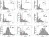 |
Fig. 4 Visible albedo distributions of asteroids classified based on MOVIS-C data. The bin size is 0.025. Each histogram shows the taxonomic group (defined in Sect. 2.2) and the number of objects (N) used. The vertical red bars indicate the
pV = 0.15 limit used for the discussion of |


4.3 Blue colors – 
The asteroids with (Y − J) ≤ 0.219, which is the value corresponding to that of the Sun, are classified as  . In the Bus-DeMeo taxonomy, the B types represent the blue end-member class and are distinctive because of their negative spectral slopes.
Objects classified as B-type asteroids present low albedo values and are mostly found in the middle and outer part of the main belt. Clark et al. (2010) divided a sample of 22 asteroids, classified as B types from their visible spectra, into three main groups, according to their NIR spectra: those with spectra similar to that of (2) Pallas; those similar to NIR spectrum of (24) Themis; and those not falling into either the Pallas or Themis group. In a later publication, de León et al. (2012) showed that, instead of three groups, the NIR spectra of asteroids classified as B type according to their visible spectra, presented a continuous shape variation from negative, blue spectral slopes to positive red slopes. This continuum in spectral slopes was also present in the sample of carbonaceous chondrites that best resembled the spectra of B-type asteroids in both papers. Objects having negative, blue spectral slopes in the NIR, i.e., those that will belong to our  considering their NIR colors, are associated with CV, CO, and CK carbonaceous chondrites. New findings about the composition of these objects are expected to be revealed by the NASA OSIRIS-Rex mission, whose primary target is the B-type near-Earth asteroid Bennu (Campins et al. 2010; Lauretta et al. 2017).
The colors computed from the reference spectra show that  is a distinct group in the (Y − J) vs. (J − Ks) color space. Based on these reference values we classified 144 asteroids in this category. The albedo was measured for 104 objects of this sample and their histogram shows two groups (Fig. 4). The largest group has a narrow distribution and a peak around pV = 0.075 ± 0.022. The second group presents a wide range of albedo values, from ~0.12 to 0.30, with a shallow peak around pV ≈ 0.15. For comparison, Mainzer et al. (2011b) found a median value of pV = 0.120 ± 0.022 for the B types with V-NIR spectral data; we note that they used only two objects. Our finding does not confirm this value; there is no peak in the albedo distribution corresponding to it. A detailed study of albedo values for asteroids classified as B types was performed by Alí-Lagoa et al. (2013). They found an average value of pV = 0.07 ± 0.03, which is in agreement with our result.
Less than half of our  sample (about 61 asteroids) are associated with asteroid families. Among these, there are 6 objects belonging to (10) Hygiea, 9 to (24) Themis, and 8 to (668) Dora. All of these correspond to our low albedo group of
  .
.
The largest portion of  associated with collisional families is of 24 objects linked to (221) Eos. This is one of the outer main belt families that has over 9000 members and it is recognized as K type (Nesvorný et al. 2015). Mothé-Diniz et al. (2008) noted spectral similarities between the Eos family asteroids and CO3, CV3, and CK carbonaceous chondrites. The albedo values are available for 16 out of these 25 objects, and its average value is pV = 0.166 ± 0.042. This is in agreement with the value of pV = 0.163 ± 0.035 reported by Masiero et al. (2015) for the Eos family.
Although it is not outlined by the colors computed from reference spectra, the albedo values and the link between some objects and the family of (221) Eos show a marginal mixture of  with possible spectrally K types that have blue NIR colors (Morate et al. 2018).
4.4 C and X complexes: Cni,
 , and
, and

Even though they are spectrally distinctive, the types corresponding to the C and X complexes span similar intervals of NIR colors values. By considering the broad compositional types, we clustered these two complexes into three groups. The Cni and  are separated mostly by the (J − Ks) with a difference less than ~0.05 mag. The
  shows a redder (Y − J) compared with the other two groups. It has to be noted that these groups show a uniform distribution over the region they occupy in the color space.
With respect to these groups, the largest number of asteroids (a total of 613) was assigned to the Cni group. Their albedo distribution (available for 481 out of these 613 objects) proved that the separation was successful. A fraction of ~ 80% are low albedo objects (pV ≤ 0.10) that are compatible with a carbonaceous-like composition. About 41% of asteroids classified in this group (196 objects) are linked to asteroid families. Among these, the largest percentage of objects belongs to (10) Hygiea and (24) Themis.
All three groups associated with the C/X complex show a double-peak distribution of albedo (Fig. 4). A first peak is centered around pV = 0.06 ± 0.02 and a second at pV ~ 0.15 ± 0.03. This last peak is more pronounced for  and
and  and can be associated with metallic compositions (Fornasier et al. 2010; Cloutis et al. 2010). We note that in Tholen taxonomy (Tholen 1984), the X complex is divided into three categories: P refers to “primitives” (low albedo objects), M refers to “metallic” (medium albedo objects, i.e., ~0.15), and E refers to “enstatites” (high albedo asteroids).
4.5  group
group
In the NIR color–color plots, the  group lies in between the S, C, and X complexes. The 665 asteroids classified as
  include many misidentifications from these three large complexes. This is outlined by their albedo distribution (Fig. 4).
We notethat about half (98 out of 214) of the asteroids classified in this group and associated with asteroid families are linked to (221) Eos (recognized as K-type family). We showed that some of the (221) Eos family members have blue colors (thus were classified as  ), but the albedo is compatible with K type. This suggests that the group covers a larger color interval than expected from the reference set.
4.6 S complex asteroids: Sni
Asteroids classified as Sni are spread over a broad region in the (Y − J),(J − Ks), and (H − Ks) color space. They cover a continuous interval of NIR colors. Using a sample of objects spectrally classified by SMASS (Xu et al. 1995; Bus & Binzel 2002b) and S3OS2 (Lazzaro et al. 2004), Popescu et al. (2016) showed that S-complex asteroids are clearly separated in the (Y− J) vs. (J − Ks) plot, forming a distinct cluster with a continuous distribution.
In this work we used the reference spectra of S, Sq, Sr, Sv, and Q types from DeMeo et al. (2009) to define our Sni group; we note that Sa was included in the  group. A total of 3315 asteroids are assigned to this group by the two algorithms. It represents more than half of the sample for which we report a taxonomic classification.
WISE albedos are available for 1882 asteroids classified as Sni. They show a Gaussian distribution with a peak at pV = 0.26 ± 0.10. This is close to the median value of pV = 0.223 ± 0.073 reported by Mainzer et al. (2011b) for asteroids belonging to the S complex according to the Bus-DeMeo taxonomy. A small fraction of asteroids (~4%) have albedo values lower than 0.10 (outliers), and are most likely misidentified D types because of the proximity of the two groups in the color–color plot (Fig. 1).
We found asteroids in the Sni group that have a variety of orbital parameters from near-Earth asteroids to outer main belt populations. A few objects identified in the Hilda and Trojan populations present albedo values do not confirm a silicate-like composition and are most likely misidentifications of D types. A notable exception is asteroid (3675) Kemstach, which we classified as Sni, and it has orbital elements that place it into Cybele population. This is known to be dominated by primitive C and D types. Our classification of (3675) Kemstach is in agreement with the albedo value of pV = 0.181 ± 0.018 and with the taxonomic type reported by SDSS. The visible spectra obtained by Lagerkvist et al. (2005) confirm its classification as an S-complex object.
About 30% (875 objects) of asteroids classified as Sni were associated with various asteroids families. In this sample, 251 out of 875 asteroids are associated with the (15) Eunomia family (a large middle main belt family dominated by the S-complex asteroids), which has more than 5000 members (Nesvorný et al. 2015).
We also note the presence of Sni asteroids in families dominated by very different compositions compared to S types, such as (4) Vesta, (93) Minerva, (135) Hertha, (158) Koronis, and (221) Eos. As noted by Licandro et al. (2017) and Morate et al. (2018), the Vesta family includes a non-negligible fraction of S types (≈11%).
4.7 Basaltic asteroids – Vni
Asteroids with (Y − J) ≥ 0.5 and (J − Ks) ≤ 0.3 were identified byLicandro et al. (2017) as V types. They found 477 V-type candidates with color magnitude errors less than 0.1. A sample of 244 of these V-type candidates are not associated with the Vesta family. As the only confirmed source of basaltic material is (4) Vesta, several dynamical mechanisms were proposed to explain the large number of basaltic asteroids outside the family (Carruba et al. 2014; Brasil et al. 2017).
We report 798 objects classified as Vni based on the updated version of the MOVIS catalog, and with a less restrictive limit for the error (Q2). About 694 objects follow the conditions of (Y − J) ≥ 0.5 and (J − Ks) ≤ 0.3. The Vni asteroids with colors outside these limits are in the vicinity of the S-complex region and lie in the continuous region in between these two groups.
The Vni group associated with basaltic asteroids shows the broadest distribution in color space, outlined in terms of mean and standard deviation values: (Y − J) = 0.632 ± 0.122, (J − Ks) = 0.060 ± 0.139, and (H − Ks) = −0.078 ± 0.172. Licandro et al. (2017) noted that the (Y − J) colors of theVesta family candidates seem to have a narrower distribution than the colors of the non-Vesta family asteroids. Visible and NIR spectral surveys (e.g., Ieva et al. 2016; Migliorini et al. 2017, 2018) of these spectrophotometric V-type candidates are required to confirm how this color variation translates into actual compositional differences.
The albedo values of asteroids classified as Vni present a broad distribution (Fig. 4) that is centered around pV = 0.352 ± 0.121. This is similar to the median value of pV = 0.362 ± 0.100 reported by Mainzer et al. (2011b) for asteroids classified as V types according to the Bus-DeMeo taxonomy. Although this is very speculative, we cannot discard the possibility that the two additional peaks at pV = 0.30 and pV = 0.23 might be indicative of two different compositional subgroups inside V types. For an in-depth analysis of V-type asteroids, please refer to Licandro et al. (2017).
5 Discussion
The taxonomy reported in this work provides a large number of asteroids classified as Sni and Vni. The number of objects compatible with the C and X complexes is only about one-quarter of those compatible with S complex. This ratio is a result of several biases introduced because of the observational limits and methods used for classification.
As a consequence of limit in the apparent magnitude of the VISTA-VHS survey, objects that have high albedo and are close to the observer have a higher probability of being observed (Jedicke et al. 2002). This introduces a bias favoring our Sni and Vni groups and the inner main belt asteroids, which have the largest percentage of rocky, S-type asteroids. The observational bias can be roughly outlined by considering the number of objects above and below the α line (see Eq. (3) from Popescu et al. 2016), which is an approximation to separate the S and V types from the B, C, X, D types. This implies a ratio of ~60% for possible detections of S and V types.
The second bias is introduced by the classification method. While the Sni and Vni groups are well defined in the color space, the  , Cni, Cg xni,
  ,
,  , and
, and  groups partially overlap at certain intervals. In most of the cases in which the borders are not well constrained (as is the case for these six groups), the two algorithms used for the classification provide different solutions and the objects are unclassified. These six groups were considered as a single cluster by Morate et al. (2018) and used to analyze the compositional distribution across the asteroids families.
A subtle bias is also introduced by the reference set used for the definition of the classes. To define X-complex types, DeMeo et al. (2009) used only 32 asteroids, 45 for C complex, and 198 for S-complex. The number of objects classified by us using MOVIS catalog follows roughly the same proportion: 91  , 197
, 197  , 613 Cni, and 3315 Sni.
About one-third (2601 out of 9097) of the objects with errors in Q2 limits were not uniquely assigned to any of the taxonomical groups. In this cases the two algorithms provided different classifications. A fraction of this unclassified sample correspond to those asteroids that have color values at the border of or in the overlapping interval between multiple groups. Most of these cases are in the region of the  , Cni, Cg xni,
  , and
, and  groups. There is also a cluster of unclassified objects between
  and
and  groups. The distribution of classified and unclassified asteroids is shown in Fig. 5.
There is a sample of unclassified objects that were not categorized in any of the groups we defined. As an example, objects with (Y − J) > 0.5 and intermediate (J − Ks) values, i.e., 0.3 < (J − Ks) ≲ 0.65, were not classified. The most likely spectral types that match these objects from the reference set are O and R types, which were not used in this study as they are defined on a single spectrum. Thus, about 218 objects fall in this category. Their distribution is widely spread in the color space.
Another set of unclassified objects (308 asteroids) lies in between the regions occupied by  ,
,  , and
, and  . This corresponds to values of (Y − J) ≤~0.3 and 0.55 < (J − Ks). These colors indicate an almost flat spectral curve in the Y and J bands that turns red beyond 1.25 μm. About ~65% of the WISEalbedo values measured for 207 out of these 308 unclassified objects are lower than 0.1. Meteoritic samples with equivalent spectral behavior are CM2 carbonaceous chondrites (Fig. 6), and in particular samples of Murchison meteorite heated at 400–500 °C. Their reflectances at 0.55 μm are comparable with the visible albedo of the asteroids.
To assess how the existing meteorites in our collections sample the asteroids compositions, we computed the synthetic (Y − J) and (J − Ks) colors for spectral data available in the RELAB database6 (Pieters & Hiroi 2004). The results are shown in Fig. 7. The asteroids distribution in the color–color space follows the same pattern as that of meteorites, but with a much broader distribution. This reflects the known fact that our meteorite records do not sample all the compositions observed in asteroids.
Near-infrared colors are efficient for identifying end-member classes such as V and A types. Also, the identified objects have albedo values in agreement with the two taxonomical classes (thus, they are less affected by observational biases). The V- and A-type candidates are considered fragments of differentiated bodies. Thus, they play a key role in understanding the accretion and geochemical evolution in the main belt (Burbine et al. 1996; Scheinberg et al. 2015; Scott et al. 2015).
The V types are associated with basaltic achondrite meteorites (e.g., McCord et al. 1970; Consolmagno & Drake 1977), which have metal-free pyroxene dominated composition and are representative for crustal material (Burbine et al. 1996). The olivine-dominated asteroids, classified as A types, are expected to be formed through magmatic differentiation (e.g., Sunshine & Pieters 1998; de León et al. 2004; Sunshine et al. 2007; Sanchez et al. 2014). Therefore, they could be mantle fragments of differentiated bodies (e.g., Burbine et al. 1996), or come from nebular processes that produce olivine-dominated objects similar to R-chondrites (Schulze et al. 1994).
Our current meteoritic evidence shows that at least 100 chondritic parent bodies in the main belt experienced partial or complete melting and differentiation before having been disrupted (Burbine et al. 1996; Sanchez et al. 2014; Scott et al. 2015, and references therein). Therefore, they should have produced a much larger number of olivine-dominated objects. The spectral surveys show a paucity of such bodies, which is known as the “missing mantle problem” or the “olivine paradox” (DeMeo et al. 2015).
The hypotheses proposed to explain the olivine paradox vary from inferring the small size of olivine-dominated asteroids (below the limit of detection), i.e., the “battered to bits” scenario (Burbine et al. 1996), to those suggesting that the classic view of asteroids differentiating into a pyroxene-rich crust, olivine-rich mantle, and iron core may be uncommon (Elkins-Tanton et al. 2011).
Our dataset allows us to quantify this problem up to a ~ 2 km size limit of the bodies. Both V and A types have prominent features, which put them in well-defined regions in (Y − J) vs. (J − Ks) color–color space. V types have approximately (Y − J) ≥ 0.5 and (J − Ks) ≤ 0.3 (Vni). A types are characterized by a red spectral slope which in terms of colors is equivalent to (J − Ks) ≥ ~0.65 ( ). Figure 5 shows a significant difference in terms of population density over the two colors regions, with V types being significantly more abundant than A types.
In orderto add more constraints to the quality of our dataset, we consider only those objects that have measured albedo pV ≥ 0.15. This allows us to identify 68 A-type (Table 3) and 338 V-type candidates, including 101 members of the Vesta family. This gives a ratio of about five times more basaltic asteroids than the olivine-dominated objects, and about four times more if the Vesta family members are not considered.
The diameters of A-type candidates range from 1.3 km for (125969) 2003 FU30 to 8 km for (4982) Bartini, with an average value of DAavg = 3.4 ± 1.4 km. The exception is (2872) Gentelec which has a diameter of 13.6 km for a pV = 0.15 ± 0.016, and it was classified as D type by Bus & Binzel (2002a), while we reported it as  . A similar average diameter value is computed for V-type candidates DVavg = 3.5 ± 4.3 km. Also, the size-frequency distributions are identical for the two classes (Fig. 8), and significantly different from S types (associated with ordinary chondrites), which have similar albedos. Therefore, the different ratio of A- and V-type candidates, and a similar size-frequency distribution of the two groups are not in favor of the two scenarios outlined by Burbine et al. (1996).
One interesting case in our dataset is asteroid (11616) 1996 BQ2, which has orbital parameters that place it in the Cybele population. Its (Y − J) = 0.37± 0.05 and (J − Ks) = 0.79 ± 0.07 colors suggest an A-type candidate. The probabilistic algorithm report it as  with a probability p = 0.93 and the kNN algorithm found it as
  with probability p = 0.58 and as
  with p = 0.42. It is classified as an S-type by Carvano et al. (2010), according to its SDSS visible photometry, and its WISE albedo is pV = 0.246 ± 0.038. The broad observational measurements make (11616) 1996 BQ2 an olivine-dominated candidate7, in a region dominated by P and D types (Gradie et al. 1989). The presence of this object may not be so unexpected since Mothé-Diniz et al. (2003) noted that the number of S-type objects near the inner side of the Hecuba gap (i.e., the 2:1 mean motion resonance with Jupiter) is low but not zero. For example, based on SDSS data, Carruba et al. (2015) reported five S types and one A type in the Cybele region. Also, Gil-Hutton & Licandro (2010) reported (11616) 1996 BQ2 as an S type and hypothesized that the presence of these objects in the Cybele population could be the result of a dynamical mechanism influencing objects in the inner border of the gap, such as migration due to the Yarkovsky effect or resonance perturbations on unstable asteroids inside the Hecuba gap.
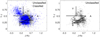 |
Fig. 5 Distribution of asteroids in the (Y − J) vs. (J − Ks) plot for asteroids with (Y − J)err ≤ 0.118 and (J − Ks)err ≤ 0.136 (asteroids with errors in Q2 limits). Left panel: the objects for which a final taxonomic class was assigned are shown in blue, while those for which the two algorithms gave a different solution are shown in gray. Right panel: for clarity, the unclassified asteroids are shown as a separate figure. |
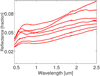 |
Fig. 6 Examples of visible to NIR reflectance spectra of CM2 carbonaceous chondrites. The reflectances are shown in absolute units (i.e., fraction of reflected light). The spectra are almost flat in Y and J bands and then turn extremely red in J and Ks bands (almost doubling their reflectance value). These types of compositions may explain the unclassified group with (Y − J) ≈ 0.3 and (J − Ks) ≥ ~ 0.6. |
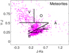 |
Fig. 7 Near-infrared colors computed from spectra of all meteorites currently available in the RELAB database. A total number of 2636 spectra was used. |
List of asteroids classified as  based on MOVIS-C NIR colors and having pV ≥ 0.15 (Mainzer et al. 2011a, 2014).
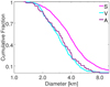 |
Fig. 8 Size-frequency distribution of asteroids classified as |

6 Future perspectives
Taxonomic classifications can also be inferred from other parameters than from spectral and spectrophotometric observations. Oszkiewicz et al. (2012) searched for correlations between the classification of asteroids and photometric phase curve using the H, G12 photometric phase function. They found that the G12 parameter provides a statistical approach to studying taxonomic classification for large population of asteroids. Belskaya et al. (2017) showed that by using polarimetric data, it is possible to refine asteroids taxonomy by distinguishing several types that cannot be identified using spectra over the visible to NIR interval. Moreover, based on the similarity of the polarization phase curves for asteroids with the same taxonomic type, they suggest that polarimetric behavior is intimately related to the surface composition.
Several surveys will provide a large amount of data in the next decade. In particular, the high-cadence multi-epoch observations of the Large Synoptic Survey Telescope (LSST Science Collaboration et al. 2009) will dramatically improve our knowledge of solar system bodies through discoveries and orbit determination (Rhodes et al. 2017). In addition to astrometric positions, the obtained photometry will allow phase curves studies for compositional types (Oszkiewicz et al. 2012) and shape modeling (Ďurech et al. 2005; Durech et al. 2015).
Spectroscopically, it is expected that a robust classification can be obtained for at least 100 000 asteroids from the low-resolution visible spectra obtained by Gaia (Delbo’ et al. 2012). Also, during their nominal execution times, the J-PLUS/S-PLUS photometric surveys, which is a joint Spanish–Brazilian project that aims to map an area of the sky of 8000 square degrees, are expected to observe tens of thousands of asteroids and measure their visible colors using a 12-filter system covering the 0.3–1.0 μm range (De Prá & Carvano 2014).
New data in the V-NIR region are also expected from Euclid survey. This is a wide-field space mission, equipped with a silicon-carbide 1.2 m aperture Korsch telescope and two instruments, a visible imaging camera, and a NIR spectrometer and photometer (Laureijs et al. 2011). By considering the current survey design, Carry (2018) have approximated that about 150 000 solar system objects, mainly from the asteroid main belt, should be observable by Euclid.
This survey will open a window onto peculiar classes of objects (i.e., small objects with high inclinations) because of its faint magnitude limit (photometrically, VAB ≈ 24.5), its spectral coverage of visible to NIR – considering spectral and spectrophotometric data, and a strategy that will avoid ecliptic latitudes and have a photometric pattern that consists in repeated sequences of four broadband filters. In particular, as shown in this paper, the use of Y and J filters provides the means to infer the main compositional groups.
Each observation method provides a piece of the puzzle for transforming the star-like appearance of the asteroids into a little world. The meaning of each observation and the information that it brings depend on the spectral characteristics that it is sampling. Inthis context, taxonomy provides a common language for discussing the asteroids compositional properties. By combining the large quantity of data provided by the surveys, an unprecedented map of the minor bodies population will be revealed.
7 Conclusions
We have inferred a taxonomic classification for the 18 265 asteroids catalogued by MOVIS using a probabilistic method and k-nearest neighbors algorithm. This database provides the largest NIR existing set of colors for solar system objects. They were obtained with Y, J, H, and Ks filters in theframework of VISTA-VHS survey, using the VHSv20161007 intermediate release.
The asteroids spectrally classified by DeMeo et al. (2009) were considered as a reference set. The 24 classes defined by Bus-DeMeo taxonomy were clustered into several groups by considering similar compositional types and their distance in the {(Y − J), (J − Ks), (H − Ks)} space. The taxonomic classification reported in this work is based on these classes.
The applied algorithms provided a taxonomic type for all objects with at least (Y − J) and (J − Ks) colors observed. The final classifications is reported for a set of 6494 asteroids that have (Y − J)err ≤ 0.118 and (J − Ks)err ≤ 0.136 and were assigned to the same taxonomical class by the kNN and probabilistic algorithms. These asteroids were distributed as follows: 144 bodies classified as  , 613 as Cni, 197 as
  , 91 as
  , 440 as
  , 665 as
  , 233 as
  , 3315 as Sni, and 798 as Vni. The superscript indicates that the classification was obtained based on NIR colors and the subscript indicates possible misidentifications with other types.
By comparing our classification with that reported by Carvano et al. (2010) based on visible colors from SDSS survey, we found a ~ 70% of matching for identifying silicaceous and carbonaceous types. We also found that the asteroid population presents a broader range of NIR colors than those computed from meteorite spectra available in the RELAB database. This points toward a wider compositional diversity of asteroids not sampled by our current meteorite records.
We reported the albedo distribution for each taxonomic group based on the data existing in WISE. By adding the albedo constraint, we found that our V- and A-type candidates have identical size-frequency distributions but a ratio of 1–5 in favor of V types. This result adds additional constraints for the hypothesis of missing mantle problem.
Taxonomic classification of asteroids catalogued by MOVIS provides the opportunity to obtain large-scale distribution for asteroidal population, to study the faint objects, and to select targets for detailed spectral investigations.
Acknowledgements
We want to especially thank S. J. Bus and F. E. DeMeo for sharing the 371 spectra they used to define the Bus-DeMeo taxonomy. This research uses spectra acquired with the NASA RELAB facility at Brown University. M.P. acknowledges support from the AYA2015-67772-R (MINECO, Spain). The work of M.P. was also supported by a grant of the Romanian National Authority for Scientific Research – UEFISCDI, project No. PN-III-P1-1.2-PCCDI-2017-0371. D.M., J.L., and J.D.L. acknowledge support from the project AYA2012-39115-C03-03 and ESP2013-47816-C4-2-P (MINECO). J.D.L. acknowledges financial support from MINECO under the 2015 Severo Ochoa Program MINECO SEV-2015-0548. D.M. gratefully acknowledges the Spanish Ministry of Economy and Competitiveness (MINECO) for the financial support received in the form of a Severo-Ochoa Ph.D. fellowship, within the Severo-Ochoa International Ph.D. Program. The work of I.L.B. was supported by a grant of the Romanian National Authority for Scientific Research – UEFISCDI, project No. PN-III-P1-1.2-PCCDI-2017-0371. We thank Dr. Michael Mommert for his constructive and helpful suggestions.
Appendix A Reference taxonomic system
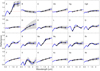 |
Fig. A.1 Template spectra (blue) and their standard deviations (gray) corresponding to taxonomic types defined by Bus-DeMeo taxonomy. Their equivalent reflectance for Y, J, H, and Ks VISTA filters are shown with black dots relative to their band centers. |
Average color values and their corresponding standard deviation of Bus-DeMeo taxonomic spectral types.
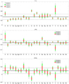 |
Fig. A.2 Average colors and standard deviations of Bus-DeMeo types computed from the 371 spectra from which the taxonomy was built. Red bars show the [–σ, +σ] interval, green bars show [–2σ, +2σ], and gray bars show [–3σ, +3σ]. The solid and dotted horizontal line represents the mean and the standard deviation of the entire set. |
References
- Alí-Lagoa, V., de León, J., Licandro, J., et al. 2013, A&A, 554, A71 [NASA ADS] [CrossRef] [EDP Sciences] [Google Scholar]
- Baudrand, A., Bec-Borsenberger, A., Borsenberger, J., & Barucci, M. A. 2001, A&A, 375, 275 [NASA ADS] [CrossRef] [EDP Sciences] [Google Scholar]
- Belskaya, I. N., Fornasier, S., Tozzi, G. P., et al. 2017, Icarus, 284, 30 [NASA ADS] [CrossRef] [Google Scholar]
- Bottke, Jr., W. F., Vokrouhlický, D., Rubincam, D. P., & Broz, M. 2002, The Effect of Yarkovsky Thermal Forces on the Dynamical Evolution of Asteroids and Meteoroids, eds. W. F. Bottke, Jr., A. Cellino, P. Paolicchi, & R. P. Binzel, 395 [Google Scholar]
- Bottke, Jr., W. F., Vokrouhlický, D., Rubincam, D. P., & Nesvorný, D. 2006, Annu. Rev. Earth Planet. Sci., 34, 157 [NASA ADS] [CrossRef] [EDP Sciences] [Google Scholar]
- Bowell, E., Chapman, C. R., Gradie, J. C., Morrison, D., & Zellner, B. 1978, Icarus, 35, 313 [NASA ADS] [CrossRef] [Google Scholar]
- Brasil, P. I. O., Roig, F., Nesvorný, D., & Carruba, V. 2017, MNRAS, 468, 1236 [NASA ADS] [CrossRef] [Google Scholar]
- Buitinck, L., Louppe, G., Blondel, M., et al. 2013, in ECML PKDD Workshop: Languages for Data Mining and Machine Learning, 108 [Google Scholar]
- Burbine, T. H., Meibom, A., & Binzel, R. P. 1996, Meteorit. Planet. Sci., 31, 607 [NASA ADS] [CrossRef] [Google Scholar]
- Bus, S. J., & Binzel, R. P. 2002a, Icarus, 158, 146 [NASA ADS] [CrossRef] [Google Scholar]
- Bus, S. J., & Binzel, R. P. 2002b, Icarus, 158, 106 [CrossRef] [Google Scholar]
- Campins, H., Morbidelli, A., Tsiganis, K., et al. 2010, ApJ, 721, L53 [NASA ADS] [CrossRef] [Google Scholar]
- Carruba, V., Huaman, M. E., Domingos, R. C., Santos, C. R. D., & Souami, D. 2014, MNRAS, 439, 3168 [NASA ADS] [CrossRef] [Google Scholar]
- Carruba, V., Nesvorný, D., Aljbaae, S., & Huaman, M. E. 2015, MNRAS, 451, 244 [NASA ADS] [CrossRef] [Google Scholar]
- Carry, B. 2018, A&A, 609, A113 [NASA ADS] [CrossRef] [EDP Sciences] [Google Scholar]
- Carry, B., Solano, E., Eggl, S., & DeMeo, F. E. 2016, Icarus, 268, 340 [NASA ADS] [CrossRef] [Google Scholar]
- Carvano, J. M., Hasselmann, P. H., Lazzaro, D., & Mothé-Diniz, T. 2010, A&A, 510, A43 [NASA ADS] [CrossRef] [EDP Sciences] [Google Scholar]
- Casagrande, L., Ramírez, I., Meléndez, J., & Asplund, M. 2012, ApJ, 761, 16 [NASA ADS] [CrossRef] [Google Scholar]
- Chapman, C. R., Morrison, D., & Zellner, B. 1975, Icarus, 25, 104 [NASA ADS] [CrossRef] [Google Scholar]
- Clark, B. E., Ziffer, J., Nesvorny, D., et al. 2010, J. Geophys. Res. (Planets), 115, E06005 [Google Scholar]
- Cloutis, E. A., Hardersen, P. S., Bish, D. L., et al. 2010, Meteorit. Planet. Sci., 45, 304 [NASA ADS] [CrossRef] [Google Scholar]
- Consolmagno, G. J., & Drake, M. J. 1977, Geochim. Cosmochim. Acta, 41, 1271 [NASA ADS] [CrossRef] [Google Scholar]
- Cross, N. J. G., Collins, R. S., Mann, R. G., et al. 2012, A&A, 548, A119 [NASA ADS] [CrossRef] [EDP Sciences] [Google Scholar]
- de León, J., Duffard, R., Licandro, J., & Lazzaro, D. 2004, A&A, 422, L59 [NASA ADS] [CrossRef] [EDP Sciences] [Google Scholar]
- de León, J., Pinilla-Alonso, N., Campins, H., Licandro, J., & Marzo, G. A. 2012, Icarus, 218, 196 [NASA ADS] [CrossRef] [Google Scholar]
- De Prá, M., & Carvano, J. 2014, in Asteroids, Comets, Meteors 2014, eds. K. Muinonen, A. Penttilä, M. Granvik, et al. Proc. Conf., 30 June–4 July, 2014, Helsinki, Finland, 450 [Google Scholar]
- Delbo’, M., Gayon-Markt, J., Busso, G., et al. 2012, Planet. Space Sci., 73, 86 [NASA ADS] [CrossRef] [Google Scholar]
- DeMeo, F. E., & Carry, B. 2013, Icarus, 226, 723 [NASA ADS] [CrossRef] [Google Scholar]
- DeMeo, F. E., & Carry, B. 2014, Nature, 505, 629 [NASA ADS] [CrossRef] [Google Scholar]
- DeMeo, F. E., Binzel, R. P., Slivan, S. M., & Bus, S. J. 2009, Icarus, 202, 160 [NASA ADS] [CrossRef] [Google Scholar]
- DeMeo, F. E., Binzel, R. P., Carry, B., Polishook, D., & Moskovitz, N. A. 2014, Icarus, 229, 392 [NASA ADS] [CrossRef] [Google Scholar]
- DeMeo, F. E., Alexander, C. M. O., Walsh, K. J., Chapman, C. R., & Binzel, R. P. 2015, Asteroids IV, eds. P. Michel, F. E. DeMeo, & W. F. Bottke (Tucson, AZ: The University of Arizona Press), 13 [Google Scholar]
- Ďurech, J., Grav, T., Jedicke, R., Denneau, L., & Kaasalainen, M. 2005, Earth Moon and Planets, 97, 179 [NASA ADS] [CrossRef] [Google Scholar]
- Durech, J., Carry, B., Delbo, M., Kaasalainen, M., & Viikinkoski, M. 2015, in Asteroids IV, eds. P. Michel, F. E. DeMeo, & W. F. Bottke (Tucson, AZ: The University of Arizona Press), 183 [Google Scholar]
- Elkins-Tanton, L. T., Weiss, B. P., & Zuber, M. T. 2011, Earth Planet. Sci. Lett., 305, 1 [NASA ADS] [CrossRef] [Google Scholar]
- Emerson, J. P., Irwin, M. J., Lewis, J., et al. 2004, in Optimizing Scientific Return for Astronomy through Information Technologies, eds. P. J. Quinn, & A. Bridger, SPIE Conf. Ser., 5493, 401 [Google Scholar]
- Fornasier, S., Clark, B. E., Dotto, E., et al. 2010, Icarus, 210, 655 [NASA ADS] [CrossRef] [Google Scholar]
- Gil-Hutton, R., & Licandro, J. 2010, Icarus, 206, 729 [NASA ADS] [CrossRef] [Google Scholar]
- Gradie, J. C., Chapman, C. R., & Tedesco, E. F. 1989, in Asteroids II (Tuscon, AZ: University of Arizona Press), 316 [Google Scholar]
- Hahn, G., & Lagerkvist, C.-I. 1988, Icarus, 74, 454 [NASA ADS] [CrossRef] [Google Scholar]
- Hambly, N. C., Mann, R. G., Bond, I., et al. 2004, in Optimizing Scientific Return for Astronomy through Information Technologies, eds. P. J. Quinn, & A. Bridger, SPIE Conf. Ser., 5493, 423 [Google Scholar]
- Hasselmann, P. H., Fulchignoni, M., Carvano, J. M., Lazzaro, D., & Barucci, M. A. 2015, A&A, 577, A147 [NASA ADS] [CrossRef] [EDP Sciences] [Google Scholar]
- Ieva, S., Dotto, E., Lazzaro, D., et al. 2016, MNRAS, 455, 2871 [NASA ADS] [CrossRef] [Google Scholar]
- Irwin, M. J., Lewis, J., Hodgkin, S., et al. 2004, Optimizing Scientific Return for Astronomy through Information Technologies, eds. P. J. Quinn & A. Bridger, SPIE Conf. Ser., 5493, 411 [Google Scholar]
- Ivezić, Ž., Tabachnik, S., Rafikov, R., et al. 2001, AJ, 122, 2749 [NASA ADS] [CrossRef] [Google Scholar]
- Jedicke, R., Larsen, J., & Spahr, T. 2002, in Asteroids III, eds. W. F. Bottke, Jr., A. Cellino, P. Paolicchi, & R. P. Binzel, 71 [Google Scholar]
- Johnson,T. V., Veeder, G. J., Loer, S. J., & Matson, D. L. 1975, ApJ, 197, 527 [NASA ADS] [CrossRef] [Google Scholar]
- Lagerkvist, C.-I., Moroz, L., Nathues, A., et al. 2005, A&A, 432, 349 [NASA ADS] [CrossRef] [EDP Sciences] [Google Scholar]
- Laureijs, R., Amiaux, J., Arduini, S., et al. 2011, ArXiv e-prints [arXiv:1110.3193] [Google Scholar]
- Lauretta, D. S., Balram-Knutson, S. S., Beshore, E., et al. 2017, Space Sci. Rev., 212, 925 [NASA ADS] [CrossRef] [Google Scholar]
- Lazzaro, D., Angeli, C. A., Carvano, J. M., et al. 2004, Icarus, 172, 179 [CrossRef] [Google Scholar]
- Levison, H. F., Bottke, W. F., Gounelle, M., et al. 2009, Nature, 460, 364 [NASA ADS] [CrossRef] [PubMed] [Google Scholar]
- Lewis, J. R., Irwin, M., & Bunclark, P. 2010, Astronomical Data Analysis Software and Systems XIX, eds. Y. Mizumoto, K.-I. Morita, & M. Ohishi, ASP Conf. Ser., 434, 91 [Google Scholar]
- Licandro, J., Popescu, M., Morate, D., & de León J. 2017, A&A, 600, A126 [NASA ADS] [CrossRef] [EDP Sciences] [Google Scholar]
- LSST Science Collaboration (Abell, P. A., et al.) 2009, ArXiv e-prints [arXiv:0912.0201] [Google Scholar]
- Mainzer, A., Grav, T., Bauer, J., et al. 2011a, ApJ, 743, 156 [NASA ADS] [CrossRef] [Google Scholar]
- Mainzer, A., Grav, T., Masiero, J., et al. 2011b, ApJ, 741, 90 [NASA ADS] [CrossRef] [Google Scholar]
- Mainzer, A., Bauer, J., Cutri, R. M., et al. 2014, ApJ, 792, 30 [NASA ADS] [CrossRef] [Google Scholar]
- Masiero, J. R., Mainzer, A. K., Grav, T., et al. 2011, ApJ, 741, 68 [NASA ADS] [CrossRef] [Google Scholar]
- Masiero, J. R., DeMeo, F. E., Kasuga, T., & Parker, A. H. 2015, in Asteroids IV, eds. P. Michel, F. E. DeMeo, & W. F. Bottke, 323 [Google Scholar]
- McCord, T. B., Adams, J. B., & Johnson, T. V. 1970, Science, 168, 1445 [NASA ADS] [CrossRef] [PubMed] [Google Scholar]
- McMahon, R. G., Banerji, M., Gonzalez, E., et al. 2013, Messenger, 154, 35 [Google Scholar]
- Migliorini, A., De Sanctis, M. C., Lazzaro, D., & Ammannito, E. 2017, MNRAS, 464, 1718 [NASA ADS] [CrossRef] [Google Scholar]
- Migliorini, A., De Sanctis, M. C., Lazzaro, D., & Ammannito, E. 2018, MNRAS, 475, 353 [Google Scholar]
- Misra, A. & Bus, S. J. 2008, Bull. Am. Astron. Soc., 40, 508 [Google Scholar]
- Mommert, M., Trilling, D. E., Borth, D., et al. 2016, AJ, 151, 98 [NASA ADS] [CrossRef] [Google Scholar]
- Morate, D., Licandro, J., Popescu, M., & de León, J. 2018, A&A, in press, DOI: 10.1051/0004-6361/201832780 [Google Scholar]
- Mothé-Diniz, T., Carvano, J. M. Á., & Lazzaro, D. 2003, Icarus, 162, 10 [NASA ADS] [CrossRef] [Google Scholar]
- Mothé-Diniz, T., Carvano, J. M., Bus, S. J., Duffard, R., & Burbine, T. H. 2008, Icarus, 195, 277 [NASA ADS] [CrossRef] [Google Scholar]
- Nesvorný, D., Brož, M., & Carruba, V. 2015, in Asteroids IV, eds. P. Michel, F. E. DeMeo, & W. F. Bottke, 297 [Google Scholar]
- Oszkiewicz, D. A., Bowell, E., Wasserman, L. H., et al. 2012, Icarus, 219, 283 [CrossRef] [Google Scholar]
- Pedregosa, F., Varoquaux, G., Gramfort, A., et al. 2011, J. Mach. Learn. Res., 12, 2825 [Google Scholar]
- Perna, D., Barucci, M. A., Fornasier, S., et al. 2010, A&A, 510, A53 [NASA ADS] [CrossRef] [EDP Sciences] [Google Scholar]
- Pieters, C. M. & Hiroi, T. 2004, in Lunar and Planetary Science Conference, eds. S. Mackwell, & E. Stansbery, 35 [Google Scholar]
- Popescu, M. 2012, Ph.D. Thesis, Observatoire de Paris; Facultatea de ?tiin?e Aplicate, Universitatea Politehnica din Bucuresti, Bucuresti, Romania [Google Scholar]
- Popescu, M., Licandro, J., Morate, D., et al. 2016, A&A, 591, A115 [NASA ADS] [CrossRef] [EDP Sciences] [Google Scholar]
- Rhodes, J., Nichol, R. C., Aubourg, É., et al. 2017, ApJS, 233, 21 [NASA ADS] [CrossRef] [Google Scholar]
- Roh, D.-G., Moon, H.-K., Shin, M.-S., Lee, H.-J., & Kim, M.-J. 2016, in AAS/Division for Planetary Sciences Meeting Abstracts, 48, 325.26 [NASA ADS] [Google Scholar]
- Sanchez, J. A., Reddy, V., Kelley, M. S., et al. 2014, Icarus, 228, 288 [NASA ADS] [CrossRef] [Google Scholar]
- Scheinberg, A., Fu, R. R., Elkins-Tanton, L. T., & Weiss, B. P. 2015, Asteroids IV, eds. P. Michel, F. E. DeMeo, & W. F. Bottke (Tucson, AZ: The University of Arizona Press), 533 [Google Scholar]
- Schulze, H., Bischoff, A., Palme, H., et al. 1994, Meteoritics, 29, 275 [NASA ADS] [CrossRef] [Google Scholar]
- Scott, E. R. D., Keil, K., Goldstein, J. I., et al. 2015, in Asteroids IV, eds. P. Michel, F. E. DeMeo, & W. F. Bottke (Tucson, AZ: The University of Arizona Press), 573 [Google Scholar]
- Sunshine, J. M. & Pieters, C. M. 1998, J. Geophys. Res., 103, 13675 [NASA ADS] [CrossRef] [Google Scholar]
- Sunshine, J. M., Bus, S. J., Corrigan, C. M., McCoy, T. J., & Burbine, T. H. 2007, Meteorit. Planet. Sci., 42, 155 [NASA ADS] [CrossRef] [Google Scholar]
- Sutherland, W., Emerson, J., Dalton, G., et al. 2015, A&A, 575, A25 [NASA ADS] [CrossRef] [EDP Sciences] [Google Scholar]
- Sykes, M. V., Cutri, R. M., Fowler, J. W., et al. 2000, Icarus, 146, 161 [NASA ADS] [CrossRef] [Google Scholar]
- Tholen, D. J. 1984, PhD Thesis (Tucson, AZ: University of Arizona) [Google Scholar]
- Veeder, G. J., Matson, D. L., & Kowal, C. 1982, AJ, 87, 834 [NASA ADS] [CrossRef] [Google Scholar]
- Veeder, G. J., Matson, D. L., & Tedesco, E. F. 1983, Icarus, 55, 177 [NASA ADS] [CrossRef] [Google Scholar]
- Xu, S., Binzel,R. P., Burbine, T. H., & Bus, S. J. 1995, Icarus, 115, 1 [NASA ADS] [CrossRef] [Google Scholar]
We have just received words of the confirmation as A type based on NIR spectral data by F. E. DeMeo and collaborators (F. E. DeMeo, priv. comm.)
All Tables
Comparison between different classification algorithms based on the leave-one-out test performed with the computed colors from the spectra used for the definition of Bus-DeMeo taxonomy.
List of asteroids classified as based on MOVIS-C NIR colors and having pV ≥ 0.15 (Mainzer et al. 2011a, 2014).
Average color values and their corresponding standard deviation of Bus-DeMeo taxonomic spectral types.
All Figures
|
Fig. 1 (Y − J) vs. (J − Ks) color–color plot derived from the 371 spectra used to define the DeMeo et al. (2009) taxonomy. The main taxonomic types are plotted with different colors for comparison. A types include A and Sa types; C and X refer to C and X complexes; S types include the S complex and Q types. We indicate the limits for each taxonomic class assumed in this work with straight lines. |
| In the text | |
|
Fig. 2 Confusion matrix for the algorithms obtained after the leave-one-out cross-validation. It shows the classes predicted by the algorithm based on their computed colors vs. the spectral classification (labeled actual class) for the 371 samples of the reference set. The top panel shows the results for the probabilistic approach and the bottom panel shows the results for the k = 3 nearest neighbors (kNN3) algorithm. Each row of the matrix represents the instances (in terms of percentages computed relative to the total number of objects for the given spectral class) in the actual spectral class, while each column represents the instances in the class predicted by the algorithm (the number of instances is given within the parenthesis). The color intensity outlines the interferences. |
| In the text | |
|
Fig. 3 Cross-tabulation matrix between the classification obtained based on MOVIS-C data (this work) and that obtained from SDSS data (Carvano et al. 2010). The percentages are specified relative to MOVIS-C assigned type, and the number of objects is specified within parenthesis. The color intensity outlines the interferences. |
| In the text | |
|
Fig. 4 Visible albedo distributions of asteroids classified based on MOVIS-C data. The bin size is 0.025. Each histogram shows the taxonomic group (defined in Sect. 2.2) and the number of objects (N) used. The vertical red bars indicate the
pV = 0.15 limit used for the discussion of |
| In the text | |
|
Fig. 5 Distribution of asteroids in the (Y − J) vs. (J − Ks) plot for asteroids with (Y − J)err ≤ 0.118 and (J − Ks)err ≤ 0.136 (asteroids with errors in Q2 limits). Left panel: the objects for which a final taxonomic class was assigned are shown in blue, while those for which the two algorithms gave a different solution are shown in gray. Right panel: for clarity, the unclassified asteroids are shown as a separate figure. |
| In the text | |
|
Fig. 6 Examples of visible to NIR reflectance spectra of CM2 carbonaceous chondrites. The reflectances are shown in absolute units (i.e., fraction of reflected light). The spectra are almost flat in Y and J bands and then turn extremely red in J and Ks bands (almost doubling their reflectance value). These types of compositions may explain the unclassified group with (Y − J) ≈ 0.3 and (J − Ks) ≥ ~ 0.6. |
| In the text | |
|
Fig. 7 Near-infrared colors computed from spectra of all meteorites currently available in the RELAB database. A total number of 2636 spectra was used. |
| In the text | |
|
Fig. 8 Size-frequency distribution of asteroids classified as |
| In the text | |
|
Fig. A.1 Template spectra (blue) and their standard deviations (gray) corresponding to taxonomic types defined by Bus-DeMeo taxonomy. Their equivalent reflectance for Y, J, H, and Ks VISTA filters are shown with black dots relative to their band centers. |
| In the text | |
|
Fig. A.2 Average colors and standard deviations of Bus-DeMeo types computed from the 371 spectra from which the taxonomy was built. Red bars show the [–σ, +σ] interval, green bars show [–2σ, +2σ], and gray bars show [–3σ, +3σ]. The solid and dotted horizontal line represents the mean and the standard deviation of the entire set. |
| In the text | |
Current usage metrics show cumulative count of Article Views (full-text article views including HTML views, PDF and ePub downloads, according to the available data) and Abstracts Views on Vision4Press platform.
Data correspond to usage on the plateform after 2015. The current usage metrics is available 48-96 hours after online publication and is updated daily on week days.
Initial download of the metrics may take a while.