| Issue |
A&A
Volume 617, September 2018
|
|
|---|---|---|
| Article Number | A28 | |
| Number of page(s) | 15 | |
| Section | Planets and planetary systems | |
| DOI | https://doi.org/10.1051/0004-6361/201832980 | |
| Published online | 12 September 2018 | |
Chemistry in disks
XI. Sulfur-bearing species as tracers of protoplanetary disk physics and chemistry: the DM Tau case
1
Max-Planck-Institut für Astronomie,
Königstuhl 17,
69117
Heidelberg, Germany
e-mail: This email address is being protected from spambots. You need JavaScript enabled to view it.
2
Department of Chemistry, Ludwig Maximilian University,
Butenandtstraße 5–13,
81377
Munich, Germany
3
INAF, Osservatorio Astrofisico di Arcetri,
Largo Enrico Fermi 5,
50125
Firenze, Italy
4
LAB, Université de Bordeaux, B18N, Allée Geoffroy,
Saint-Hilaire, 50023,
33615
Pessac Cedex, France
5
CNRS, Université de Bordeaux, B18N, Allée Geoffroy,
Saint-Hilaire, 50023,
33615
Pessac Cedex, France
6
Department of Astronomy, University of Michigan, 1085 S. University Avenue,
Ann Arbor,
MI 48109, USA
7
IRAM,
300 Rue de la Piscine,
38046
Saint-Martin-d’Hères, France
Received:
7
March
2018
Accepted:
19
June
2018
Abstract
Context. Several sulfur-bearing molecules are observed in the interstellar medium and in comets, in strong contrast to protoplanetary disks where only CS, H2CS, and SO have been detected so far.
Aims. We combine observations and chemical models to constrain the sulfur abundances and their sensitivity to physical and chemical conditions in the DM Tau protoplanetary disk.
Methods. We obtained 0.5′′ Atacama Large Millimeter Array observations of DM Tau in Bands 4 and 6 in lines of CS, SO, SO2, OCS, CCS, H2CS, and H2S, achieving a ~5 mJy sensitivity. Using the non-Local Thermodynamical Equilibrium radiative transfer code RADEX and the forward-modeling tool DiskFit, disk-averaged CS column densities and upper limits for the other species were derived.
Results. Only CS was detected with a derived column density of ~2−6 × 1012 cm−2. We report a first tentative detection of SO2 in DM Tau. The upper limits range between ~1011 and 1014 cm−2 for the other S-bearing species. The best-fit chemical model matching these values requires a gas-phase C/O ratio of ≳1 at r ≳ 50−100 au. With chemical modeling we demonstrate that sulfur-bearing species could be robust tracers of the gas-phase C/O ratio, surface reaction rates, grain size and UV intensities.
Conclusions. The lack of detections of a variety of sulfur-bearing molecules in DM Tau other than CS implies a dearth of reactive sulfur in the gas phase, either through efficient freeze-out or because most of the elemental sulfur is in other large species, as found in comets. The inferred high CS/SO and CS/SO2 ratios require a non-solar C/O gas-phase ratio of ≳1, consistent with the recent observations of hydrocarbon rings in DM Tau. The stronger depletion of oxygen-bearing S-species compared to CS is likely linked to the low observed abundances of gaseous water in DM Tau and points to a removal mechanism of oxygen from the gas.
Key words: astrochemistry / protoplanetary disks / radio lines: planetary systems / radio lines: stars / circumstellar matter
© ESO 2018
1 Introduction
One of the most exciting topics in astronomy is to understand the physical and chemical link between various stages of the star and planet formation processes and the properties of planetary systems and exoplanet atmospheres (e.g., Mordasini et al. 2012; Mollière et al. 2015; Cridland et al. 2017). Infrared and (sub-)millimeter observations of the dust continuum and molecular lines are used to study these environments. The compact, ≲100−1000 au sizes and the low, ≲0.01−0.1 M⊙ gas masses make such studies particularly challenging for protoplanetary disks, even with the most powerful observational facilities like Atacama Large Millimeter Array (ALMA), NOrthern Extended Millimeter Array (NOEMA), and the Extended Very Large Array (EVLA). Thus, compared to more than 200 molecules discovered in the interstellar medium (ISM)1, only ~20 species and their isotopologues were detected in disks (see e.g., Henning & Semenov 2013; Dutrey et al. 2014; Bergin et al. 2015).
Using this limited set of molecular tracers, crucial information about disk physics, chemistry, and kinematics at outer radii of ≳ 50−100 au has been obtained. From the relatively easy-to-detect CO isotopologues disk orientations, sizes, temperature structures, and indirect disk gas masses have been derived (e.g., Williams & Best 2014; Ansdell et al. 2016, 2017; Guilloteau et al. 2016; Pascucci et al. 2016; Schwarz et al. 2016; Long et al. 2017). More reliable gas mass measurements using HD have been obtained with Herschel forTW Hya, DM Tau, and GM Aur (Bergin et al. 2013; McClure et al. 2016; Trapman et al. 2017). The importance of CO-regulated ice chemistry for the synthesis of complex organic molecules has been supported by the H2 CO observations of DM Tau (Loomis et al. 2015) and CH3OH observationsof TW Hya (Walsh et al. 2016; Parfenov et al. 2017).
One of the most intriguing ALMA results is evidence of substantial depletion of elemental C and O in T Tauri disks, with C/O becoming >1 in a molecular layer (Bergin et al. 2016; Öberg & Bergin 2016). Schwarz et al. (2016) and Kama et al. (2016) have found that CO is depleted by two orders of magnitude in the TW Hya disk, which cannot be solely explained by the CO freeze-out in the midplane, while the CO depletion in the warmer Herbig Ae disk HD 100546 is negligible (Kama et al. 2016). Similarly, McClure et al. (2016) derived CO depletion of up to a factor of five for DM Tau and up to a factor of ~ 100 for GM Aur. Plausible mechanisms for this depletion are: 1) warm surface chemistry that converts volatile CO to less volatile CO2, 2) He+ destruction of CO, which liberates carbon that is converted into refractory complex organics, or 3) preferential removal of oxygen from the disk molecular layer by the freeze-out of water onto sedimenting large dust grains (e.g., Semenov & Wiebe 2011; Favre et al. 2013; Krijt et al. 2016; Öberg & Bergin 2016; Rab et al. 2017a). The higher freeze-out temperature of water, Tfr ~ 140−160 K, favors its depletion over the volatile CO (Tfr ~ 20−25 K) and N2 (Tfr ≤ 16−18 K) (Mumma & Charnley 2011; Qi et al. 2013; Du et al. 2015; Öberg & Bergin 2016; Krijt et al. 2016).
Despite these promising results, almost nothing is known about the sulfur content in disks. So far, only CS has been detected in dozens of disks and SO has only been detected in several younger, actively accreting disks including the disk of the Herbig A0 star AB Aur and Class I sources (Dutrey et al. 2011; Guilloteau et al. 2016; Pacheco-Vázquez et al. 2016; Sakai et al. 2016). Dutrey et al. (2011) could not detect the SO and H2 S lines with the IRAM 30-m in LkCa15, DM Tau, GO Tau, and MWC 480. They performed a careful analysis of the previously observed CS lines and the upper limits of the SO column densities and concluded that the best-fit model requires a C/O ratio of 1.2, yet this model failed to reproduce the H2S upper limits by at least one order of magnitude. The CS emission in TW Hya reveals a complex radial distribution with a surface density gap at around 95 au and low turbulent velocities (Teague et al. 2016, 2017). Using the IRAM 30-m antenna, Chapillon et al. (2012a) observed CCS in DM Tau and MWC 480 and obtained upper limits on the CCS column densities in these disks, ≲ 1.5 × 1012 cm−2. Recently, H2CS was found in the Herbig Ae disk of MWC 480 by Loomis et al. (2017; priv. comm.), where CS was also detected. Finally, Booth et al. (2018) have recently detected SO emission in HD 100546 that does not come solely from the Keplerian disk, but shows an additional non-disk component (a disk wind, a warp, or shocked gas).
This is in contrast to the studies of the ISM, where sulfur-bearing species are commonly observed and used as tracers of chemical ages (e.g., CCS/NH3; Suzuki et al. 1992), temperature/shocks (SO, SO2, OCS; Esplugues et al. 2014), X-ray irradiation (SO; Stäuber et al. 2005), grain processing (SO/H2S, SO/SO2; Charnley 1997), and turbulent transport (CCS/CO; Semenov & Wiebe 2011). The S-bearing molecules such as H2 S, SO, SO2, CS, CS2, H2 CS, S polymers, and other complex S-bearing chains and organics were detected in comets and satellites of Jovian planets in our solar system (e.g., Boissier et al. 2007; Le Roy et al. 2015; Calmonte et al. 2016). Recently, sulfur-bearing species have been detected in the molecular disk around the late-type Sun-like AGB star (Kervella et al. 2016).
The sulfur-bearing amino acids cysteine and methionine, as well as OCS acting as a catalyst in peptide synthesis, play an important role in biochemistry and hence sulfur chemistry could be related to the origin of life (Brosnan & Brosnan 2006; Chen et al. 2015). In order to make progress in our understanding of the importance of the delivery of S-bearing molecules to early Earth and Earth-like planets, a better understanding of the sulfur content of protoplanetary disks is required. Intriguingly, modern astrochemical models cannot fully reproduce the observed abundances or upper limits of sulfur-bearing species. The main reasons are likely uncertainties in the reaction rates, missing key formation routes, or unaccounted major reservoirs of sulfur (see e.g., Druard & Wakelam 2012; Loison et al. 2012; Vidal et al. 2017).
The main goals of this paper are twofold. First, we aim to study in detail sulfur chemistry in the DM Tau disk using ALMA observationsthat are several times more sensitive than the previous observations. Second, we aim to investigate the sensitivity of the disk sulfur chemistry to various physical and chemical parameters, using an appropriate DM Tau physical–chemical model. The paper is organized as follows. In Sect. 2 our ALMA Cycle 3 observationsare presented. Disk-averaged column densities and upper limits are derived in Sect. 3. In Sects. 4.1 and 4.2 the adopted physical and chemical models of the DM Tau disk are described, and the parameter space to be calculated is presented. The comparison between the observed values and the grid of DM Tau models is discussed in Sect. 5. Discussion and conclusions follow.
2 Observations
2.1 ALMA observations and data reduction
Observations of DM Tau were carried out with ALMA on June 22 (in Band 6) and July 26, 2016 (in Band 4) as part of the ALMA project 2015.1.00296.S, PI: Dmitry Semenov. The phase tracking center was αJ2000 = 04h33m48. s747, δJ2000 = 18° 10′09′′.585. The systemic velocity of the source was set to vLSR = 6 km s−1. More specifically, Band 4 data were taken with 45 antennas and baselines from 15.1 m up to 1.1 km with an on-source time of about 2 min. The Band 4 spectral setup consisted of six spectral windows with 480 channels each with a channel width of 122.07 kHz (~ 0.3 km s−1), covering about 0.4 GHz between 145.926 and 159.010 GHz, and one continuum spectral window with the 2 GHz bandwidth (128 × 15.625 MHz channels) centered at 145.021 GHz. The quasars J0510+1800 and J0431+2037 were used as bandpass, flux, and phase calibrators. The Band 6 data were taken with 37 antennas and baselines from 15.1 up to 704.1 m with an on-source time of about 20 min, using J0510+1800 and J0423–0120 as bandpass, flux, and phase calibrators. The Band 6 spectral setup consisted of three spectral windows with 240 channels each with a channel width of 244.141 kHz (~ 0.3 km s−1), covering about 0.2 GHz between 215.195 and 218.936 GHz, and one continuum spectral window with the 2 GHz bandwidth (128 × 15.625 MHz channels) centered at 232.012 GHz.
Data reduction and continuum subtraction in the uv-space were performed through the Common Astronomy Software Applications (CASA) software (McMullin et al. 2007), version 4.5.3. The continuum image at 145.021 GHz was self-calibrated, and the solutions were applied to the lines observed in Band 4 in order to improve the signal-to-noise ratio (S/N), in particular for the SO2 transitions. To further optimize the sensitivity, data from Bands 4 and 6 were cleaned using the “natural” weighting. The resulting synthesized beam size is 0.61′′ × 0.58′′ at a positional angle of ~ 28° for the 145 GHz continuum image, with the 1σ rms of 7.6 × 10⁻⁵ Jy beam−1. For the line images at Bands 4 and 6 the synthesized beams are similar, ≈ 0.6′′ × 0.5′′ (positional angle is 23°), with a spectral resolution of ~ 0.3 km s−1 and a 1σ rms sensitivity of 5 × 10⁻³ Jy beam−1.
Spectroscopic line parameters.
2.2 Line imaging
The targeted molecular lines, their frequencies, and spectroscopic parameters are listed in Table 1. The only detected emission (>3σ) visible in the continuum-subtracted integrated intensity and spectral maps was CS (3 − 2) (see Figs. 1 and 2). Both maps are relatively noisy because the ALMA Band 4 integration time was short, only about 2 min on-source. The observed line parameters assuming a source size of 4′′, which is estimated from the CS integrated emission map over the line profile, are presented in Table 2.
To increase the signal, we applied the pixel deprojection and azimuthal averaging technique as presented in Teague et al. (2016), Yen et al. (2016), and Matrà et al. (2017). For deprojection we used an inclination angle of −34°, a positional angle of 27°, a distance of 140 pc, and a stellar mass of 0.55 M⊙ (Teague et al. 2015; Simon et al. 2017). After such deprojection, a double-peaked spectrum typical for Keplerian disks becomes a single-peaked spectrum with a narrower line width. The resulting shifted spectra are presented in Fig. 3 for Band 4 and in Fig. 4 for Band 6, respectively. As can be clearly seen, the only firmly detected line in our dataset is CS (3 − 2), with a peak S/N ≳ 14. There is a tentative detection of the SO2 (32,2 − 31,3) line, with a peak S/N ≈ 4.7, albeit the signal is slightly shifted from the velocity center by + 1 km s−1 (Fig. 3, left bottom panel). The rest of the lines are not detected.
3 Observed CS column density and the upper limits for SO, SO2, H2S, OCS, and CCS
3.1 Fitting with RADEX
Since we are mainly dealing with non-detections, and our CS data are noisy, we decided to start with a simple approach based on Fedele et al. (2012, 2013) to derive disk-averaged vertical column densities or their upper limits. The ALMA data in the CASA format were exported as FITS files and analyzed in GILDAS software2. Each individual integrated spectrum was fitted with a Gaussian function, assuming a source diameter of 4′′ (560 au at a distance of 140 pc), based on the CS 0th-moment map (see Table 2). To convert line fluxes to column densities, we employed a widely used RADEX code3 (van der Tak et al. 2007). The code uses a uniform physical structure to perform line radiative transfer with the Large Velocity Gradient (LVG) method based on statistical equilibrium calculations with collisional and radiative processes and background radiation. Optical depth effects are accounted for with an escape probability method. The molecular data were taken from the Leiden Atomic and Molecular Database (LAMDA4; see Schöier et al. 2005). A local line width of 0.14 km s−1 was assumed for all molecules based on the previous CS observations by Guilloteau et al. (2012). When two transitions were observed, they were both stacked and taken into account.
By varying excitation temperature, volume density, and column density, the χ2 values between the observed and modeled CS line fluxes were computed and minimized. The upper limits of the column densities of the other non-detected sulfur-bearing species were derived in a similar manner, using the observed 3σ rms as the line flux limit. We were not able to analyze the CCS data as there are no collisional rate data in the LAMDA and Basecol5 databases. The resulting χ2 distributions for the assumed volume densities of 106, 107, and 108 cm−3 representative of the outer DM Tau molecular layer are shown in Fig. 5.
The computed χ2 distributions do not depend on the assumed gas density since we have chosen the most easily excited and strong transitions for our observations. The only exception is H2 S (22,0 − 21,1), which is slightly better fitted with the high-volume density of 108 cm−2. Due to their low upper state energies Eu < 20 K (Table 1), the temperature dependence of the CS and SO2 fits is rather flat, with the best-fit values of Tex ≲ 100 K. The higher upper state energies of the H2S (22,0 − 21,1), OCS (18 − 17), and SO (3Σ v = 0, 55 − 44) transitions are 84, 100, and 44 K, respectively, which makes them sensitive to the temperature and leads to a prominent temperature dependence of their χ2 distributions (Fig. 5). The best-fit temperatures and column densities (or their upper limits) are summarized in Table 3.
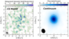 |
Fig. 1 Left panel: ALMA Band 4 CS (3 − 2) 0th-moment map of the DM Tau disk. Right panel: dust continuum map of the DM Tau disk at 146.969 GHz. The first contours and the level steps are at 3σ rms. |
 |
Fig. 2 ALMA Band 4 spectral map showing CS (3 − 2) in the DM Tau disk. The channel spacing is 0.3 km s−1. The first contour and the level step are at 3σ rms. |
Line parameters for the observed sulfur-bearing transitions towards DM Tau.
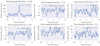 |
Fig. 3 Pixel deprojected and azimuthally averaged ALMA Band 4 spectra showing CS (3 − 2), CCS (N = 12 − 11, J = 13 − 12), OCS (12 − 11), SO (3 Σ v = 0, 34 − 23), SO2 (v = 0, 42,2 − 41,3), and SO2 (v = 0, 32,2 − 31,3) spectral windows in DM Tau. |
 |
Fig. 4 Pixel deprojected and azimuthally averaged ALMA Band 6 spectra showing H2 S (22,0 − 21,1), OCS (18 − 17), and SO (3Σ v = 0, 55 − 44) spectral windows in DM Tau. |
3.2 Parametric fitting with DiskFit
As the next step, we performed a more elaborate analysis of the data using our DiskFit parametric method (see Piétu et al. 2007; Dutrey et al. 2011; Teague et al. 2015). The disk structure is parameterized by radial power laws for the surface density, temperature, kinematics, and molecular column density, which are fitted with a combination of χ2 minimization and Markov chain Monte Carlo (MCMC) of the observed visibilities in the uv-plane. DiskFit firstfinds the systemic velocity, the geometrical parameters of the disk system (position of the center, inclination and positional angles, radius of emission), and the disk rotation profile. Next, the dust continuum emission is fitted and dust parameters are obtained. Finally, gas surface density, scale height, temperature, micro-turbulent velocity, and column density distribution are derived.
To increase the S/N of the CS spectrum, the ALMA data were merged with our previous CS (3 − 2) IRAM 30-mdata (Dutrey et al. 2011). Neglecting the primary beam correction, which is justified for our ~ 4′′ emission source, the two visibility sets were merged after resampling in velocity to the coarsest spectral resolution. For the analysis in DiskFit, we used both datasets at their native spectral resolution and fitted them assuming the same underlying physical model. While this approach does not provide a better line image, it preserves the full information on the line widths at the highest possible accuracy. To analyze the non-detected lines we used the best-fit temperature and the radial profiles from the merged CS data. Finally, to get more accurate upper limits for the column densities of SO, SO2, and OCS, we stacked each of their pairs of observed transitions together (see Figs. 3 and 4). The DiskFit results at a representative outer disk radius of 300 au are given in Table 3.
As can be clearly seen, while the CS column densities derived by both methods are comparable, ~ 2−6 × 1012 cm−2, the RADEX-based approach cannot constrain CS excitation temperature, as only one transition of CS was observed. The more advanced DiskFit approach is able to recover radial gradients and points to rather cold CS excitation temperatures of ≈ 10 K in the outer DM Tau disk at ~300 au. This is consistent with the low, ~7−15 K, excitation temperatures for CO, CCH, CN, HCN, and CS estimated by Piétu et al. (2007), Henning et al. (2010), Chapillon et al. (2012b), and Guilloteau et al. (2012). The further differences between the methods are mainly due to a) differences in the underlying modeling assumptions, where RADEX fits the disk-averaged quantities while DiskFit recovers radial gradients, and b) a left-over degeneracy between the inferred temperature and column density, where both “cold; high-column density” and “warm; low-column density” solutions could exist. For further theoretical analysis of these results in Sect. 5, it is essential that both RADEX and DiskFit converge to a similar best-fit column density ratio for CS/SO of ≳ 1−3.
 |
Fig. 5 Computed χ2 distributionswith RADEX code for three volume densities of 106, 107, and 108 cm−3 and varied Tex and molecular column densities N. Top to bottom: results for CS, H2S, SO, SO2, and OCS aredepicted. The red contours indicate the χ2-minima. |
Best-fit temperatures and column densities or 3σ upper limits obtained with RADEX and DiskFit.
4 Modeling
4.1 Disk physical structure
The DM Tau physical disk model is based on a 1+1D steady-state α-model similar to that of D’Alessio et al. (1999), where equal gas and dust temperatures are assumed. This flaring model was extensively used in our previous studies of DM Tau-like disk chemistry (e.g., Henning et al. 2010; Semenov & Wiebe 2011). The assumption of equal dust and gas temperatures is reasonably accurate for the molecular layers of S-bearing species that do not extend very high into the disk atmosphere (see, e.g., Woitke et al. 2009; Akimkin et al. 2013). The disk model has an outer radius of 800 au, an accretion rate of 5 × 10⁻⁹ M⊙ yr−1, a viscosity parameter α = 0.01, and a total gas mass of 0.066 M⊙ (Dutrey et al. 2007; Henning et al. 2010; Semenov & Wiebe 2011). This value is close to the upper value of the DM Tau disk mass, 4.7 × 10⁻² M⊙, inferred from the HD Herschel observations by McClure et al. (2016).
The Shakura–Sunyaev parametrization (Shakura & Sunyaev 1973) of the turbulent viscosity ν was adopted:
 (1)
(1)
where H(r) is the disk pressure scale height, cs is the sound speed, and α = 0.01 is the dimensionless parameter.
To model turbulent transport along with disk chemical evolution, we used the standard description of the diffusivity coefficient,
 (2)
(2)
where Sc is the Schmidt number that describes the efficiency of turbulent diffusivity (see e.g., Schräpler & Henning 2004; Semenov & Wiebe 2011). We considered three regimes of mixing, namely, laminar disk with no mixing (Sc = ∞), “slow” mixing (Sc = 100), and “fast” mixing (Sc = 1). Diffusion of ices is treated similarly to the gas-phase molecules. The calculated thermal and density structure of the disk is shown in Fig. 6.
4.2 Disk chemical model
The adopted chemical model is based on the public gas-grain ALCHEMIC code6 (see Semenov et al. 2010; Semenov & Wiebe 2011). The chemical network is based on the osu.2007 ratefile with recent updates to the reaction rates from the Kinetic Database for Astrochemistry (KIDA; Wakelam et al. 2012).
To calculate ultaviolet (UV) ionization and dissociation rates, the mean far-UV intensity at a given disk location is obtained by summing the stellar UV flux  and interstellar UV flux χIS = 1−100χ0, which are scaled down by the visual extinction in the radial and vertical directions, respectively. We used the interstellar UV radiation field χ0 of Draine (1978). Several tens of photoreaction rates are adopted from van Dishoeck et al. (2006)7. The self-shielding of H2 from photodissociation is calculated by Eq. (37) from Draine & Bertoldi (1996). The shielding of CO by dust grains, H2, and the CO self-shielding is calculated using a precomputed table of Lee et al. (1996; Table 11).
The stellar X-ray radiation is modeled using Eqs. (4), (7)–(9) from Glassgold et al. (1997a,b), with an exponent n =2.81, a cross section at 1 keV of σ−22 = 0.85 × 10⁻²² cm2, and total X-ray luminosity of LXR = 1031 erg s−1. The X-ray emitting source is assumed to be 12 stellar radii above the star. This makes X-ray ionization dominate over the cosmic ray (CR) ionization in the disk molecular layer. The standard CR ionization rate is assumed to be ζCR = 1.3 × 10⁻¹⁷ s−1. Ionization due to the decay of short-living radionuclides (SLR) is taken into account, with the SLR ionization rate of ζRN = 6.5 × 10⁻¹⁹ s−1 (Finocchi et al. 1997).
The gas–grain interactions include the sticking of neutral species and electrons to dust grains with 100% probability and desorption of ices by thermal, CRP-, and UV-driven processes. Uniform amorphous silicate particles of olivine stoichiometry were used, with a density of 3 g cm−3 and a radius of 0.1 μm. Each grain provides 1.88 × 10⁶ surface sites for surface recombinations (Biham et al. 2001), which proceed through the Langmuir–Hinshelwood mechanism (e.g., Hasegawa et al. 1992). The UV photodesorption yield of 10−5 was adopted (Cruz-Diaz et al. 2016; Bertin et al. 2016). Photodissociation processes of solid species are taken from Garrod & Herbst (2006) and Semenov & Wiebe (2011). We assumed a 1% probability for chemical desorption (Garrod et al. 2007; Vasyunin & Herbst 2013). The standard rate equation approach to the surface chemistry was utilized. Overall, the disk chemical network consists of 654 species made of 12 elements, including dust grains, and 7299 reactions.
The age of the DM Tau system is ~3–7 Myr (Simon et al. 2000); we used 5 Myr in the chemical simulations. The “low metals” elemental abundances of Graedel et al. (1982), Lee et al. (1998), and Agúndez & Wakelam (2013) were utilized (see Table 4). Parameters of the “standard” (or reference) DM Tau disk model are summarized in Table 5.
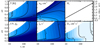 |
Fig. 6 Adopted DM Tau disk physical structure. Top row, left to right panels: spatial distributions of the gas and dust temperature (Kelvin), the gas density (cm−3; log10 scale), and the pressure scale height (au; log10 scale). Bottom row, left to right panels: UV intensity (in χ0 units of the Draine 1978 interstellar FUV field), the combined ionization rate due to CRPs, stellar X-rays, and short-lived radionuclides (s−1), and the turbulent diffusion coefficient (cm2 s−1; log10 scale). |
Initial abundances used for the DM Tau chemical modeling.
5 Results
Using the DM Tau disk physical and chemical model presented above, we performed about 20 detailed chemical calculations by varying various physical and chemical parameters as shown in Table 6. The results are compared to the reference model summarized in Table 5. The computed abundances of sulfur species at 5 Myr were vertically integrated to obtain radial distributions of the column densities. After that, medians of these column densities were computed at radii between 100 and 800 au and compared with the best-fit disk-averaged quantities derived with RADEX and the best-fit values at the radius of 300 au derived with DiskFit (see Figs. 7–14 and related discussion).
The key result of our study is that the observed CS column density and the sensitive upper limits for other S-bearing species can only be matched when the gas has a non-solar metallicity with a C/O ratio of ≈ 1 (see Fig. 14). Another favorable model has a solar C/O ratio of 0.46 but requires a rather low X-ray luminosity of ≲ 1029 erg s−1, and a low initial sulfur abundance of ≲10−8 (Fig. 11). In all the other cases the observed and modeled CS/SO ratios disagree.
Another key result of our modeling is that a combination of sulfur-bearing molecules, if detected in disks, could provide very useful and unique diagnostics of a variety of disk physical and chemical processes. The summary of which sulfur-bearing species and what ratios are sensitive to what specific disk physical and chemical parameters is presented in Table 7. The CS/SO and CS/SO2 ratios are mainly sensitive to the local gas-phase C/O elemental ratio. The presence of abundant SO and SO2 in the gas indicates either their more efficient surface synthesis via fast diffusivity of S, O, and other heavy radicals, or more efficient release of SO, SO2 ices into thegas phase (shocks, high-energy irradiation, turbulent transport). In ideal circumstances when H2 S, OCS, and H2CS could also be observed in a disk, one could even determine which process is dominating.
Parameters of the standard DM Tau disk model.
 |
Fig. 7 Theobserved and computed median column densities of the key sulfur-bearing species at r = 100−800 au in the DM Tau disk at 5 Myr are compared. Cross indicates the CS column density and the arrows indicate the upper limits of the observed column densities for other S-bearing molecules. Left to right panels: three scenarios of turbulent mixing are considered: (1) laminar disk (Sc = ∞), (2) slow mixing (Sc = 100), and (3) fast mixing (Sc = 1; Semenov & Wiebe 2011). |
5.1 Impact of turbulent mixing
The turbulent transport in disks enriches chemistry by bringing chemical ingredients from cold and dark outer regions to those where reactions with barriers, ice evaporation, and mild high-energy processing of gas and ices become active (see e.g., Ilgner et al. 2004; Heinzeller et al. 2011; Semenov & Wiebe 2011; Furuya & Aikawa 2014). This is particularly true for refractory ices and/or species produced at least partly by surface reactions, including sulfurette molecules. As a result of transport, all sulfur species show a uniform increase in column densities by ≲ 3−10, especially when the mixing is fast (see Fig. 7). Consequently, such an uniform increase does not strongly affect the computed CS/SO ratio, which remains similar in the laminar (CS/SO ≈ 0.026) and the fast turbulent mixing (CS/SO ≈ 0.044) cases. Both these values are too low compared with our observations showing CS/SO ≳ 1.
 |
Fig. 8 As Fig. 7 but for sulfur initial elemental abundances. The cross indicates the CS column density and the arrows indicate the upper limits of the observed column densities for other S-bearing molecules. Left to right panels: three sets of initial elemental sulfur abundances are considered: (1) X(S) =9 × 10⁻⁹, (2) X(S) = 9 × 10⁻⁸, and (3) X(S) = 9 × 10⁻⁷. |
 |
Fig. 9 As Fig. 7 but for surface diffusivities. The cross indicates the CS column density and the arrows indicate the upper limits of the observed column densities for other S-bearing molecules. Left to right panels: three scenarios for the surface diffusivity are considered: (1) slow diffusion, Ediff ∕Ebind = 0.77, (2) average diffusion, Ediff∕Ebind = 0.5, and (3) fast diffusion, Ediff∕Ebind = 0.3. |
5.2 Impact of initial sulfur abundances
Another crucial factor that has an impact on the outcome of sulfur chemistry is the total amount of elemental sulfur available for chemistry. The higher the initial sulfur elemental abundance that is not locked inside dust grains, the higher the computed abundances and column densities for the sulfur molecules and ices. The response of disk sulfur chemistry to the linear increase of the initial sulfur elemental abundance in our model is almost linear (see Fig. 8). This again means that the resulting CS/SO ratio remains too low, ~ 0.02, as compared to our interferometric observationsshowing CS/SO ≳ 1.
5.3 Impact of surface diffusivities
Unlike the previous two parameters, the pace of surface chemistry regulated by the surface diffusivities affects the disk sulfur chemistry differently (Fig. 9). The molecules SO2, OCS, and to a lesser degree SO can be efficiently produced via surface processes involving S, O, CO, or SO only when these heavy ices are mobile and hence benefit from the fast, Ediff∕Ebind = 0.3, diffusion. The H2S that is also produced on grains does not benefit that much from faster diffusivities because it is formed via direct hydrogenation of S and H atoms can rapidly scan the dust surfaces even at T =10−20 K and when the assumed diffusivity is slow, Ediff∕Ebind = 0.77. Other S-bearing species show two distinct trends. While CS and partly SO, synthesized mainly in the gas phase, are not strongly affected by the pace of surface chemistry, the column densities of C2 S and H2 CS decline when the surface diffusivities increase. For these two species the decline is caused by the competition between the two main C-reservoirs, CO and CH4. The synthesis of CH4 greatly benefits from faster diffusion, which lowers gas-phase abundances of other simple hydrocarbons like CH and CH3, out of which C2S and H2CS are produced. As above, the modeled CS/SO ratios when the surface diffusivities are varied remain too low compared to the observations.
Grid of DM Tau models computed by varying key disk physical and chemical parameters.
Sulfur-bearing tracers of outer disk parameters.
5.4 Impact of grain growth
The main effect of grain growth on disk chemistry, when the total dust/gas ratio does not severely change, is the reduction of the grain surface available for accretion (per unit gas volume). The disk sulfur chemistry reacts to the uniform grain growth from the ISM-like 0.1 μm-sized grains to the 10 μm-sized grains by increasing abundances and column densities of nearly all S-species due to their less severe freeze-out and more efficient gas-phase chemistry with S, particularly for SO and SO2 (see Fig. 10). The only species that shows an opposite trend is H2 S, whose column densities decrease by a small factor of two (from 8 × 1012 cm−2 to 4 × 1012 cm−2) with grain growth. This species is produced almost entirely by the surface hydrogenation of sulfur and its production efficiency suffers from the reduced grain surface available for this process. Grain growth, as the other disk parameters discussed above, does not bring the modeled CS/SO ratios of ≈ 0.026, ≈ 0.018, and ≈ 0.009 (for the 0.1, 1, and 10 μm-sized grains, respectively) to the observed value of ≳ 1.
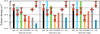 |
Fig. 10 As Fig. 7 but for grain sizes. The cross indicates the CS column density and the arrows indicate the upper limits of the observed column densities for other S-bearing molecules. Left to right: three uniform dust grain sizes are considered: (1) 0.1 μm, (2) 1 μm, and (3) 10 μm. |
 |
Fig. 11 As Fig. 7 but for stellar X-ray luminosities. The cross indicates the CS column density and the arrows indicate the upper limits of the observed column densities for other S-bearing molecules. Left to right panels: three cases of stellar X-ray luminosities are considered: (1) LX= 1031 erg s−1, (2) LX = 1030 erg s−1, and (3) LX = 1029 erg s−1. |
5.5 Impact of stellar X-ray luminosity
The change of the stellar X-ray luminosity affects chemistry differently for CS and SO and other sulfur species (see Fig. 11). When the adopted LX decreases from 1031 to 1029 erg s−1, the corresponding CS column densities increase from ≈4 × 10¹¹ to 3 × 1012 cm−2. In contrast to this, the SO column densities decrease by a factor of two from ≈ 1.5 × 10¹³ to ~ 8 × 1012 cm−2. The SO abundances decrease with decreasing X-ray ionization rate because 1) less SO molecules can be kicked out from dust grain surfaces and2) because less oxygen can be liberated from O-bearing ices and from gaseous CO upon destruction by the X-ray-produced He+ ions. The CS, in contrast, benefits from extra carbon liberated from CO by He+.
Consequently, the modeled CS/SO ratio increases from ≈ 0.026 to 0.43, getting closer to the observedvalue of ≳1. The observed CS column density and the SO upper limits derived with DiskFit are matched with the model with the “standard” S elemental abundance of 9 × 10⁻⁸ (Table 4). In contrast, in order to better match the absolute values of the observed CS column density and the SO upper limits derived with RADEX, the model with the low stellar X-ray luminosity of 1029 erg s−1 needs an additional downscaling of the initial sulfur elemental abundance by a factor of five, to the value of ≈ 2 × 10⁻⁸.
This is the first model that fits the data and the observed CS/SO ratio, although the best-fit stellar X-ray luminosity of 1029 erg s−1 seems to be too low compared to the observed X-ray properties of DM Tau. Based on the X-ray measurements with Chandra and XMM in the range of 0.3−10 keV, the quiescent stellar X-ray luminosity of DM Tau is about 1030 erg s−1 (M. Guedel, priv. comm.), and can temporarily rise during the flares. This value is close to the median value representative of the X-ray luminosities measured in T Tauri stars, 1029 −1031 erg s−1 (e.g., Feigelson & Montmerle 1999; Telleschi et al. 2007). In the previous chemical studies of the DM Tau disk, comparable values of 2− 100 × 1029 erg s−1 were used (Semenov & Wiebe 2011; Cleeves et al. 2014; Teague et al. 2015; Bergin et al. 2016; Rab et al. 2017b).
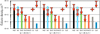 |
Fig. 12 As Fig. 7 but for cosmic ray ionization rates. The cross indicates the CS column density and the arrows indicate the upper limits of the observed column densities for other S-bearing molecules. Left to right panels: three CRP ionization rates were considered: (1) ζCRP = 1.3 × 10⁻¹⁸ s−1, (2) ζCRP = 1.3 × 10⁻¹⁷ s−1, and (3) ζCRP = 1.3 × 10⁻¹⁶ s−1. |
5.6 Impact of cosmic ray ionization
The impact of the CR ionization rate on the disk sulfur chemistry is relatively minimal (see Fig. 12). The most affected species, H2 CS, shows an increase in the column densities from 6 × 10¹¹ to ≈ 1012 cm−2 for the lowand high CRP ionization rates of 1.3 × 10⁻¹⁸ s−1 and 1.3 × 10⁻¹⁶ s−1, respectively. As we mentioned in the Sect. 4.2, in our disk model the X-ray-driven ionization dominates over the CRP ionization in the disk molecular layer, where gaseous sulfur-bearing molecules have peak abundances. Thus, by varying CRP ionization rates the modeled CS/SO ratios remain too low, ≲ 0.035, compared to the observed value of ≳ 1.
 |
Fig. 13 As Fig. 7 but for interstellar UV radiation fields. The cross indicates the CS column density and the arrows indicate the upper limits of the observed column densities for other S-bearing molecules. Left to right panels: three cases of the interstellar UV radiation field are considered: (1) 1χ0, (2) 10χ0, and (3) 100χ0, where χ0 is the Draine (1978) IS UV field. |
5.7 Impact of interstellar UV radiation
The interstellar UV radiation regulates photodissociation and photoionization of gas as well as photodesorption and photoprocessing of ices. The key process for the chemistry in the disk molecular layer is photodesorption of ices. When more UV radiation penetrates into this layer, it liberates refractory ices more efficiently, increasing their gas-phase concentrations. In addition, more energetic UV-irradiation of ices creates reactive radicals including O and S, boosting the surface synthesis of chemically-related molecular ices.
This is what can be seen in Fig. 13. The heavy molecules that are mainly synthesized on grains, like SO2, OCS, and H2 S, show higher column densities by factors of ~4−25 for the case when the IS UV field is χUV = 100χ0 compared tothe standard χUV = 1χ0 case. In contrast, CS, H2CS, and CCS are produced mainly in the gas phase and hence their abundances are not that sensitive to changes of the UV radiation intensity. Consequently, by increasing the amount of the UV radiation penetrating into the DM Tau molecular layer, the resulting CS/SO ratios can only become lower, from ≈ 0.026 for the χUV = 1χ0 model to ≈ 0.004 for the χUV = 100χ0 model.
5.8 Impact of C/O ratios
One of the most important parameters shaping the entire disk chemistry is the total elemental C/O ratio, as well as the degree of carbon and oxygen depletion. As soon as the C/O ratio switches from < 1 to > 1, the abundances of many oxygen-bearing species drop substantially, as the majority of elemental O becomes locked in CO. In contrast, the concentrations of carbon-bearing species increase due to the availability of elemental C that is not bound in CO. This makes the CS/SO and CS/SO2 ratios extremely sensitive to the local disk C/O ratio (see Fig. 14).
The column densities of SO and SO2 in our DM Tau model drop by factors of ~100 and 500, respectively, when the C/O ratio changes from 0.46 to 1.2. In contrast, the column densities of CS, CCS, and H2 CS are increased by factors of ~ 100, 35, 2, respectively. The column densities of H2 S do not change as it contains neither C nor O. The column densities of OCS also do not strongly change because this molecule has an efficient surface formation route via CO + S, and hence follows the CO evolution.
As a result, the modeled CS/SO ratio increases from the “standard” low value of ≈ 0.026 (C/O = 0.46) to the values of 13 (C/O = 1.0) and 282 (C/O = 1.2). The trend continues with increasing C/O ratio: for C/O = 2 the modeled CS/SO ratio is 498. As can be clearly seen in Fig. 14, the modeled and observed data agree reasonably well (taking modeling uncertainties of a factor of approximately three to ten into account).
 |
Fig. 14 As Fig. 7 but for elemental C/O ratios. The cross indicates the CS column density and the arrows indicate the upper limits of the observed column densities for other S-bearing molecules. Left to right panels: three elemental C/O ratios are modeled: (1) the solar C/O ratio of 0.46, (2) the C/O ratio of 1.0, and (3) the C/O ratio of 1.2. |
5.9 Analysis of sulfur chemistry
We used ourchemical analysis software to identify the key gas-phase and surface formation and destruction pathways for CS, SO, SO2, OCS, and H2S at a representative outer disk radius of 230 au of the “standard” DM Tau model with the solar C/O elemental composition, as in Semenov & Wiebe (2011). At this radius the temperature ranges between ≈ 9 and 50 K, the gas density is between ≈75 and 2.2 × 108 cm−3, and the visual extinction ranges between 0 and 62 magnitudes. We should note that freeze-out and desorption processes are considered in the chemical modeling, but are not listed in Table A.1.
The sulfur chemistry in outer disk regions begins with S+ reacting with light hydrocarbons such as CH3, CH4, C2 H, C3 H, producing HCS+, HC3S+, C2 S+, or C3 S+ ions, respectively. The light hydrocarbons are rapidly formed via gas-phase chemistry of C+ and later almost entirely converted to CO or freeze out. The sulfur-bearing ions dissociatively recombine with electrons, producing smaller neutral sulfurette molecules. Other slower initial formation routes involve barrierless neutral–neutral reactions with atomic sulfur, for example, S + CH, OH, CH2, or C2, forming CS or SO. At later times, the evolution of sulfur-bearing species is governed by a closed cycle where protonation processes (via HCO+, H3 O+, H ) are equilibrated by the dissociative recombination reactions, and, for some species, by gas-grain interactions and surface chemistry. In the following we describe disk chemistry for the individual sulfur-bearing molecules in detail.
The chemical evolution of CS proceeds essentially in the gas phase. The molecule CS is synthesized by dissociative recombination of C2 S+, C3 S+, HCS+, HC2S+, and H3 CS+, and by slower neutral–neutral reactions S + CH, CH2, or C2 and, later, by the SO + C reaction. The major destruction pathways are freeze-out (T ≲ 30 K), slow neutral–neutral reaction CS + CH → C2S + H, charge transfer with ionized hydrogen atoms, and protonation reactions (see Table A.1).
In contrast, the chemical evolution of H2S is governed by the surface processes. The key reaction for H2 S is the surface hydrogenation of HS followed by desorption. In turn, HS ice can be produced by the hydrogenation of surface S atoms, or by the freeze-out of the gaseous HS formed via the S + OH reaction. The major destruction pathways for H2 S is freeze-out onto dust surfaces (at T ≲ 40−45 K), charge transfer reaction with atomic hydrogen, destruction via ion–molecule reaction with C+, and protonation reactions.
The chemical evolution of SO and SO2 is tightly linked and occurs in the gas and ice phases. The sulfur monoxide SO is produced by the slow oxidation of S, neutral–neutral reactions between S and OH and O with HS, and surface reactions between oxygen and S or HS ices. The molecule SO is mainly destroyed by exothermic neutral–neutral reactions with O, C, OH, freeze-out (T ≲ 40 K), charge transfer reactions with atomic hydrogen, and protonation reactions.
Sulfur dioxide SO2 is synthesized by the neutral–neutral reactions between SO and OH, slow radiative association of SO and O, and the same SO + O reaction occurring on the dust surfaces. The SO2 major removal channels are freeze-out at T≲60−80 K, ion–molecule reaction with C+ and neutral–neutral reaction with C, and protonation reactions.
Finally, the chemical evolution of OCS begins with the oxidation of HCS and radiative association of S and CO. The molecule OCS can also be produced by the surface recombination of S and CO as well as CS and O ices. The removal of OCS includes freeze-out (T ≲ 45 K), destruction via ion–molecule reaction with C+, charge transfer reactions with H atoms, and protonation reactions.
6 Discussion
6.1 Comparison with previous studies of sulfur chemistry
While manysulfur-bearing species have been routinely observed in low-mass star-forming regions, the previous searches have found only very few S-bearing species in disks, mostly CS (e.g., Dutrey et al. 2014). One of the first detailed studies of the sulfur chemistry around LkCa 15, MWC 480, DM Tauri, and GO Tauri, using the IRAM 30-m antenna and the gas-grain NAUTILUS chemical code, was performed by Dutrey et al. (2011). No H2 S 11.0 − 10,1 emission at 168.8 GHz and SO 22,3 − 11,2 emission at 99.3 GHz were detected. The comprehensive analysis of the upper limits for SO and the detected CS emission pointed to an elemental C/O ratio of 1.2, albeit that the H2 S upper limits were not reproduced, suggesting that either H2S remains locked onto grain surfaces or reacts with other species.
Our results agree with these finding, as our best-fit model also requires an elemental C/O ratio of ≳ 1 in the molecular layer of the DM Tau disk (see Fig. 14). In this scenario almost all of the oxygen is bound in CO and too little O is available for synthesis of other O-bearing species, including SO and SO2. We cannot constrain the C/O ratio in the molecular layer more accurately due to the non-detection of SO and SO2 and other S-bearing species and the poorly known abundance of elemental sulfur available for disk chemistry. Unlike in Dutrey et al. (2011), our sensitive upper limit of the H2S column density is well explained by all models except the model with high elemental sulfur abundance or high UV intensity (see Figs. 8 and 13). Our modeling shows that the H2 S abundance is not sensitive to other disk physical and chemical properties (see Table 7).
Thus, the combination of CS, SO, or SO2, and H2S lines (or very stringent upper limits) may allow us in the future to more reliably constrain both the C/O ratio and the sulfur elemental abundance in the molecular layers of disks with well-known physical structure.
In addition, our models can explain the upper limits of the H2 S column density, where the previous study by Dutrey et al. (2011) failed to reproduce it. To find the reason for this discrepancy, we first compared the gas-phase and grain surface networks that were used in Dutrey et al. (2011) and found that they are fairly similar. Next, the gas-phase abundance and column density of H2 S in the outer part of the DM Tau disk is controlled by the freeze-out and desorption and thus is sensitive to the adopted disk temperature structure. Dutrey et al. (2011) used a two-layered parametric disk model and considered a representative radius of 300 au. At that radius, the midplane has a temperature of 10 K and extends vertically up to z∕Hr ≈ 1.5. Above the midplane, a molecular layer with a temperature of ~17 K begins. In comparison, in our disk model at r = 300 au the midplane has a temperature of 12 K and extends vertically up to z∕Hr ≈ 1, after which a warmer molecular layer begins (with temperatures up to ~ 30−40 K). Finally, we present the median H2S column densities over the outer 100−800 au region. In fact, in our DM Tau model the H2S column densities increase toward the outer edge of the disk, and at r = 300 au the typical values of N(H2S) are about 1013 – a few times 1013 cm−2. These valuesare comparable with the values at r = 300 au calculated by Dutrey et al. (2011), given the modeling uncertainties of several factors.
Guilloteau et al. (2013) performed a chemical survey of 42 T Tauri and Herbig Ae systems located in the Taurus–Auriga region with the IRAM 30 m antenna (one hour/source integration), including the SO emission line. They detected SO in seven sources, which also showed strong H2CO emission. The observed SO line profiles suggest that the emission is coming from outflows or envelopes rather than from Keplerian rotating disks. Later, Guilloteau et al. (2016) performed a deeper survey of 30 disks in Taurus–Auriga with the IRAM 30 m antenna (with about one hour/source integration), targeting two SO lines. In addition to many CS detections, they detected SO in four T Tauri and Herbig Ae sources, which traces predominantly outflow or shocked regions.
The SO molecule has also been detected and imaged in the transitional disk around the Herbig A0 star AB Aur by Pacheco-Vázquez et al. (2016). They found that the SO emission has a ring-like shape and that SO is likely depleted from the gas phase in the horseshoe-shaped dust trap in the inner disk. Recently, Booth et al. (2018) detected two SO 7 − 6 emission lines in the HD 100546 disk at around 300 GHz and found that the SO emission does not come solely from the Keplerian disk, but likely traces either a disk wind, an inner disk warp (seen in CO emission), or an accretion shock from a circumplanetary disk associated with the proposed protoplanet embedded in the disk at 50 au.
Indeed, SO and SO2 are widely used as shock tracers in the studies of high-mass star-forming regions or low-mass Class 0 and I protostars and bipolar outflows associated with the low mass stars (Pineau des Forets et al. 1993; Tafalla et al. 2010; Esplugues et al. 2014; Gerner et al. 2014). Recently, Podio et al. (2015) observed SO emission rings around the Class 0 protostars L1527 and HH212, which likely trace shocked gas at the disk-envelope interface. As we have shown in Sect. 5.9, SO and SO2 are partly produced via dust surface process and remain frozen at T ≲ 45−80 K, while CS is produced in the gas phase and is more volatile, with an evaporation temperature of ~ 30 K. Thus, shocks or elevated temperatures available in the inner, r ≲ 30−100 au regions of T Tauri disks are required to effectively put SO and SO2 ices back into the gas phase, while in the outer disks SO and SO2 desorption is less efficient and driven by CRP-induced or interstellar UV photons. Apparently, this is not the case for the quiescent DM Tau disk (or, at least, its outermost regions).
6.2 The non-solar C/O ratios in disks as traced by CS/SO
Our main finding is that the observed data are best explained by a C/O ratio greater than one. This agrees well with the other recent observational results. Bergin et al. (2016) have observed C2 H in both TW Hya and DM Tau with ALMA, and also found cyclic C3 H2 in TW Hya. These hydrocarbons show bright emission rings arising at the edge of the millimeter-sized dust disk, which can only be reproduced in the chemical models with a C/O ratio > 1 and a strong UVfield in molecular layers, as in our study. They explained the effect of non-solar C/O ratios in the molecular layer by predominant removal of oxygen in the form of water ice into the dark and cold midplane by the sedimentation of large, pebble-sizeddust grains. This leads to a stratified C/O structure in the disk with higher ratios within the UV-dominated upper layer and solar-like C/O ratios in the ice-rich disk midplane.
A similar result was obtained by Kama et al. (2016), who have observed the CI, OI, C2 H, CO, and CII lines to constrain the carbon and oxygen abundances in TW Hya and HD 100546. To match the observations, a strong depletion of the C and O reservoirs in the cold T Tauri disk around TW Hya is required, but the warmer disk around HD 100546 is much less depleted. Both disks, however, needed a model with C/O > 1 in order to match the observations. The strong C and O depletion in TW Hya has also been confirmed by the CO isotopologue observations and detailedmodeling of Schwarz et al. (2016). McClure et al. (2016) have also found a moderate C and O depletion in DM Tau and a strong depletion of the C and O reservoirs in GM Aur. The authors proposed a mechanism of locking the refractory O-rich ices (like H2 O) by the sedimentation of grains into the dark midplane where it cannot easily desorb back into the gas phase.
This mechanism of volatile depletion in disks has been investigated by Du et al. (2015) and Krijt et al. (2016). Du et al. (2015) have proposed that the elemental C and O abundances can be reduced in the upper layers of the outer disk as major C- and O-bearing volatiles reside mainly at the midplane, locked up in the icy mantles of millimeter-sized dust grains partly decoupled from the gas, which hence cannot be transported upward by turbulence. Krijt et al. (2016) have developed a dynamical model of evolving dust grains in a disk. They found that dust coagulation enhanced by the presence of ice mantles benefits dust growth and hence dust vertical settling, leading to a strong depletion of water in the disk atmosphere, where the gas-phase C/O becomes ~ 1 and higher. Thisremoval mechanism is supported by the previous dynamical studies of evolving dust grains in disks and laboratory experiments (e.g., Birnstiel et al. 2010; Piso et al. 2015; Musiolik et al. 2016).
An alternative explanation has been proposed by Favre et al. (2013). They obtained a low disk-averaged gas-phase CO abundance in TW Hya and inferred that this could be due to chemical destruction of CO by the X-ray-produced He+ ions, followed by rapid formation of heavy carbon chains that freeze-out onto dust grains, while oxygen goes into the synthesis of other species, like CO2, water, or complex organic molecules. In our disk chemical model the destruction of CO by the X-ray-produced He+ ions occurs only in the upper layers at r ≲ 3−10 au and hence cannot explain the derived C/O ratio of ≳1 from our sulfur data probing the outer, >100 au region of the DM Tau disk.
6.3 Sulfur chemistry as tracer of water snowline in disks
A defining feature for planet formation is the water snowline that shapes the properties of emerging planets (Birnstiel et al. 2016). It is temperature-, pressure-, and composition-dependent, and has a value of T ~ 140−160 K, which corresponds to the radial distances of ~1−3 au in a typical T Tauri disk (van Dishoeck et al. 2014). Condensation of water is connected to the C/O ratio of gas and ices in protoplanetary disks (Bergin et al. 2015; Öberg & Bergin 2016). Despite its importance to protoplanetary disk evolution and planet formation, a direct detection of the water snowline in protoplanetary disks is still missing.
While the chemical modeling of the DM Tau disk presented above was mainly focused on the interpretation of the outer-disk averaged sulfur chemistry, our model shows another interesting result, namely, a close relationship between the column densities of H2 S, SO2, and H2 O in the inner disk region at <10 au (Fig. 15). Specifically, a three-orders-of-magnitude rise in the column density of SO2 is observed starting at ~4−5 au, which is at a distance about two times larger than the snowline location of ~ 2−2.5 au. The rise in SO2 prior to and inside the snowline is caused by the faster surface synthesis due to increased grain temperatures and more rapid thermal hopping and desorption of water ice that brings oxygen back to the gas phase and enables faster SO2 gas-phase chemistry. The molecule H2S shows the opposite trend, with a rapid decrease in column density of six orders of magnitude inside the snowline. This is due to the fact that H2S forms efficiently on dust grains, which formation is effective only at low temperatures of ≲ 20−40 K and limited by hydrogen residence time on grains. At higher temperatures sulfur surface chemistry begins to produce heavier O-bearing sulfur species like SO2 and OCS. Potentially, these chemical trends will be able to be observed in inner disk regions with the forthcoming JWST mission.
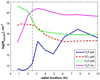 |
Fig. 15 Our DM Tau chemical model suggests a relationship between the column densities of H2 S, SO2, and H2 O. The black vertical line marks the snowline location at ~2.5. |
7 Conclusions
We have performed a new search for the sulfur-bearing molecules CS, SO, SO2, OCS, CCS, H2CS, and H2S in the DM Tau disk with ALMA in Cycle 3. We have detected CS and have a tentative SO2 detection. Failure to detect sulfur-bearing molecules in DM Tau other than CS implies either efficient freeze-out of H2 S, SO, SO2, and OCS or thatthis sulfur is bound in other species, possibly refractory compounds as identified in comets. For the data analysis, we merged the new CS (3 − 2) ALMA Cycle 3 data with our previous PdBI data and stacked the two transitions for SO, SO2, and OCS. We employed a one-dimensional (1D) non-LTE radiative transfer code RADEX to obtain the disk-averaged CS column densities and the upper limits for the other sulfurette molecules. Also, we used a 1+1D forward-modeling tool DiskFit to derive the corresponding radial distributions. Both these methods show that the CS column density is ~ 2−6 × 1012 cm−2 (with a factor of two uncertainty).
These observed values have been compared with a suite of detailed physical–chemical models of the DM Tau disk by varying key parameters such as the elemental sulfur abundance, grain sizes, amount of high-energy radiation, turbulent mixing, C/O ratios, and surface chemistry efficiency. We found that the observed data and, in particular, the CS/SO ratio of ≳ 1, can only be reliably explained by a disk modelwith a C/O ratio of ≳1, in agreement with the previous studies of the sulfur content of protoplanetary disks. This is also consistent with the recent observations of bright hydrocarbon emission rings and non-solar C/O ≳ 1 ratios found in DM Tau, TW Hya, and a few other disks. The stronger depletion of oxygen-bearing S-species compared to CS is likely linked to the proposed removal mechanism of oxygen from the disk upper layers by growing and sedimenting ice-coated grains. Furthermore, our chemical modeling demonstrated that sulfur-bearing species, if more were detected in disks, could be robust tracers of other key disk properties, such as efficiency of surface reactions, grain sizes, and amount of high-energy radiation that is able to reach the disk molecular layers. Thus more sensitive observations of sulfur-bearing molecules in the disks with well-studied structures are required with ALMA and NOEMA facilities.
Acknowledgements
This paper makes use of the following ALMA data: ADS/JAO.ALMA#2015.1.00296.S. ALMA is a partnership of ESO (representing its member states), NSF (USA), and NINS (Japan), together with NRC (Canada) and NSC and ASIAA (Taiwan) and KASI (Republic of Korea), in cooperation with the Republic of Chile. The Joint ALMA Observatory is operated by ESO, auI/NRAO, and NAOJ. This work was supported by the National Programs PCMI and PNPS from INSU-CNRS. DS acknowledges support from the Heidelberg Institute of Theoretical Studies for the project “Chemical kinetics models and visualization tools: Bridging biology and astronomy”. DF and CF acknowledge support from the Italian Ministry of Education, Universities and Research, project SIR (RBSI14ZRHR). This research made use of NASA’s Astrophysics Data System. The figures in this paper were constructed with the MATPLOTLIB package (Hunter 2007) and APLPY package hosted at http://aplpy.github.io.
Appendix A Additional table
Key chemical processes for S-bearing species.
References
- Agúndez, M., & Wakelam, V. 2013, Chem. Rev., 113, 8710 [CrossRef] [PubMed] [Google Scholar]
- Akimkin, V., Zhukovska, S., Wiebe, D., et al. 2013, ApJ, 766, 8 [NASA ADS] [CrossRef] [Google Scholar]
- Ansdell, M., Williams, J. P., van der Marel, N., et al. 2016, ApJ, 828, 46 [Google Scholar]
- Ansdell, M., Williams, J. P., Manara, C. F., et al. 2017, AJ, 153, 240 [NASA ADS] [CrossRef] [EDP Sciences] [Google Scholar]
- Bergin, E. A., Cleeves, L. I., Gorti, U., et al. 2013, Nature, 493, 644 [NASA ADS] [CrossRef] [PubMed] [Google Scholar]
- Bergin, E., Blake, G., Ciesla, F., Hirschmann, M., & Li, J. 2015, PNAS, 112, 8965 [Google Scholar]
- Bergin, E. A., Du, F., Cleeves, L. I., et al. 2016, ApJ, 831, 101 [NASA ADS] [CrossRef] [Google Scholar]
- Bertin, M., Romanzin, C., Doronin, M., et al. 2016, ApJ, 817, L12 [NASA ADS] [CrossRef] [Google Scholar]
- Biham, O., Furman, I., Pirronello, V., & Vidali, G. 2001, ApJ, 553, 595 [NASA ADS] [CrossRef] [Google Scholar]
- Birnstiel, T., Dullemond, C. P., & Brauer, F. 2010, A&A, 513, A79 [NASA ADS] [CrossRef] [EDP Sciences] [Google Scholar]
- Birnstiel, T., Fang, M., & Johansen, A. 2016, Space Sci. Rev., 205, 41 [NASA ADS] [CrossRef] [Google Scholar]
- Boissier, J., Bockelée-Morvan, D., Biver, N., et al. 2007, A&A, 475, 1131 [NASA ADS] [CrossRef] [EDP Sciences] [Google Scholar]
- Booth, A., Walsh, C., Kama, M., et al. 2018, A&A, 611, A16 [NASA ADS] [CrossRef] [EDP Sciences] [Google Scholar]
- Brosnan, J. T., & Brosnan, M. E. 2006, J. Nutr., 136, 1636S [CrossRef] [Google Scholar]
- Calmonte, U., Altwegg, K., Balsiger, H., et al. 2016, MNRAS, 462, S253 [CrossRef] [Google Scholar]
- Chapillon, E., Dutrey, A., Guilloteau, S., et al. 2012a, ApJ, 756, 58 [NASA ADS] [CrossRef] [Google Scholar]
- Chapillon, E., Guilloteau, S., Dutrey, A., Piétu, V., & Guélin, M. 2012b, A&A, 537, A60 [NASA ADS] [CrossRef] [EDP Sciences] [Google Scholar]
- Charnley, S. B. 1997, ApJ, 481, 396 [NASA ADS] [CrossRef] [Google Scholar]
- Chen, Y.-J., Juang, K.-J., Nuevo, M., et al. 2015, ApJ, 798, 80 [NASA ADS] [CrossRef] [Google Scholar]
- Cleeves, L. I., Bergin, E. A., & Adams, F. C. 2014, ApJ, 794, 123 [NASA ADS] [CrossRef] [Google Scholar]
- Cridland, A. J., Pudritz, R. E., Birnstiel, T., Cleeves, L. I., & Bergin, E. A. 2017, MNRAS, 469, 3910 [NASA ADS] [CrossRef] [Google Scholar]
- Cruz-Diaz, G. A., Martín-Doménech, R., Muñoz Caro, G. M., & Chen, Y.-J. 2016, A&A, 592, A68 [NASA ADS] [CrossRef] [EDP Sciences] [Google Scholar]
- D’Alessio, P., Calvet, N., Hartmann, L., Lizano, S., & Cantó, J. 1999, ApJ, 527, 893 [NASA ADS] [CrossRef] [Google Scholar]
- Draine, B. T. 1978, ApJS, 36, 595 [NASA ADS] [CrossRef] [Google Scholar]
- Draine, B. T., & Bertoldi, F. 1996, ApJ, 468, 269 [NASA ADS] [CrossRef] [EDP Sciences] [Google Scholar]
- Druard, C., & Wakelam, V. 2012, MNRAS, 426, 354 [NASA ADS] [CrossRef] [Google Scholar]
- Du, F., Bergin, E. A., & Hogerheijde, M. R. 2015, ApJ, 807, L32 [NASA ADS] [CrossRef] [Google Scholar]
- Dutrey, A., Henning, T., Guilloteau, S., et al. 2007, A&A, 464, 615 [NASA ADS] [CrossRef] [EDP Sciences] [Google Scholar]
- Dutrey, A., Wakelam, V., Boehler, Y., et al. 2011, A&A, 535, A104 [NASA ADS] [CrossRef] [EDP Sciences] [Google Scholar]
- Dutrey, A., Semenov, D., Chapillon, E., et al. 2014, Protostars and Planets VI (Tucson: University of Arizona Press), 317 [Google Scholar]
- Esplugues, G. B., Viti, S., Goicoechea, J. R., & Cernicharo, J. 2014, A&A, 567, A95 [NASA ADS] [CrossRef] [EDP Sciences] [Google Scholar]
- Favre, C., Cleeves, L. I., Bergin, E. A., Qi, C., & Blake, G. A. 2013, ApJ, 776, L38 [NASA ADS] [CrossRef] [Google Scholar]
- Fedele, D., Bruderer, S., van Dishoeck, E. F., et al. 2012, A&A, 544, L9 [Google Scholar]
- Fedele, D., Bruderer, S., van Dishoeck, E. F., et al. 2013, A&A, 559, A77 [NASA ADS] [CrossRef] [EDP Sciences] [Google Scholar]
- Feigelson, E. D., & Montmerle, T. 1999, ARA&A, 37, 363 [NASA ADS] [CrossRef] [Google Scholar]
- Finocchi, F., Gail, H.-P., & Duschl, W. J. 1997, A&A, 325, 1264 [NASA ADS] [Google Scholar]
- Furuya, K., & Aikawa, Y. 2014, ApJ, 790, 97 [NASA ADS] [CrossRef] [Google Scholar]
- Garrod, R. T., & Herbst, E. 2006, A&A, 457, 927 [NASA ADS] [CrossRef] [EDP Sciences] [Google Scholar]
- Garrod, R. T., Wakelam, V., & Herbst, E. 2007, A&A, 467, 1103 [NASA ADS] [CrossRef] [EDP Sciences] [Google Scholar]
- Gerner, T., Beuther, H., Semenov, D., et al. 2014, A&A, 563, A97 [NASA ADS] [CrossRef] [EDP Sciences] [Google Scholar]
- Glassgold, A. E., Najita, J., & Igea, J. 1997a, ApJ, 480, 344 [NASA ADS] [CrossRef] [Google Scholar]
- Glassgold, A. E., Najita, J., & Igea, J. 1997b, ApJ, 485, 920 [NASA ADS] [CrossRef] [Google Scholar]
- Graedel, T. E., Langer, W. D., & Frerking, M. A. 1982, ApJS, 48, 321 [NASA ADS] [CrossRef] [Google Scholar]
- Guilloteau, S., Dutrey, A., Wakelam, V., et al. 2012, A&A, 548, A70 [NASA ADS] [CrossRef] [EDP Sciences] [Google Scholar]
- Guilloteau, S., Di Folco, E., Dutrey, A., et al. 2013, A&A, 549, A92 [NASA ADS] [CrossRef] [EDP Sciences] [Google Scholar]
- Guilloteau, S., Reboussin, L., Dutrey, A., et al. 2016, A&A, 592, A124 [NASA ADS] [CrossRef] [EDP Sciences] [Google Scholar]
- Hasegawa, T. I., Herbst, E., & Leung, C. M. 1992, ApJS, 82, 167 [NASA ADS] [CrossRef] [Google Scholar]
- Heinzeller, D., Nomura, H., Walsh, C., & Millar, T. J. 2011, ApJ, 731, 115 [NASA ADS] [CrossRef] [Google Scholar]
- Henning, T., & Semenov, D. 2013, Chem. Rev., 113, 9016 [Google Scholar]
- Henning, T., Semenov, D., Guilloteau, S., et al. 2010, ApJ, 714, 1511 [NASA ADS] [CrossRef] [Google Scholar]
- Hunter, J. D. 2007, Comput. Sci. Eng., 9, 90 [Google Scholar]
- Ilgner, M., Henning, T., Markwick, A. J., & Millar, T. J. 2004, A&A, 415, 643 [NASA ADS] [CrossRef] [EDP Sciences] [Google Scholar]
- Kama, M., Bruderer, S., van Dishoeck, E. F., et al. 2016, A&A, 592, A83 [NASA ADS] [CrossRef] [EDP Sciences] [Google Scholar]
- Kervella, P., Homan, W., Richards, A. M. S., et al. 2016, A&A, 596, A92 [NASA ADS] [CrossRef] [EDP Sciences] [Google Scholar]
- Krijt, S., Ciesla, F. J., & Bergin, E. A. 2016, ApJ, 833, 285 [NASA ADS] [CrossRef] [Google Scholar]
- Lee, H.-H., Herbst, E., Pineau des Forêts, G., Roueff, E., & Le Bourlot, J. 1996, A&A, 311, 690 [NASA ADS] [Google Scholar]
- Lee, H.-H., Roueff, E., Pineau des Forets, G., et al. 1998, A&A, 334, 1047 [NASA ADS] [Google Scholar]
- Le Roy, L., Altwegg, K., Balsiger, H., et al. 2015, A&A, 583, A1 [Google Scholar]
- Loison, J.-C., Halvick, P., Bergeat, A., Hickson, K. M., & Wakelam, V. 2012, MNRAS, 421, 1476 [NASA ADS] [CrossRef] [Google Scholar]
- Long, F., Herczeg, G. J., Pascucci, I., et al. 2017, ApJ, 844, 99 [NASA ADS] [CrossRef] [Google Scholar]
- Loomis, R. A., Cleeves, L. Ilsedore, Öberg, K. I., Guzman, V. V., & Andrews, S. M. 2015, ApJ, 809, L25 [NASA ADS] [CrossRef] [Google Scholar]
- Matrà, L., MacGregor, M. A., Kalas, P., et al. 2017, ApJ, 842, 9 [NASA ADS] [CrossRef] [Google Scholar]
- McClure, M. K., Bergin, E. A., Cleeves, L. I., et al. 2016, ApJ, 831, 167 [NASA ADS] [CrossRef] [Google Scholar]
- McMullin, J. P., Waters, B., Schiebel, D., Young, W., & Golap, K. 2007, in Astronomical Data Analysis Software and Systems XVI, eds. R. A. Shaw, F. Hill, & D. J. Bell, ASP Conf. Ser., 376, 127 [NASA ADS] [Google Scholar]
- Mollière, P., van Boekel, R., Dullemond, C., Henning, T., & Mordasini, C. 2015, ApJ, 813, 47 [NASA ADS] [CrossRef] [Google Scholar]
- Mordasini, C., Alibert, Y., Benz, W., Klahr, H., & Henning, T. 2012, A&A, 541, A97 [NASA ADS] [CrossRef] [EDP Sciences] [Google Scholar]
- Müller, H. S. P., Schlöder, F., Stutzki, J., & Winnewisser, G. 2005, J. Mol. Struct., 742, 215 [NASA ADS] [CrossRef] [Google Scholar]
- Mumma, M. J., & Charnley, S. B. 2011, ARA&A, 49, 471 [NASA ADS] [CrossRef] [Google Scholar]
- Musiolik, G., Teiser, J., Jankowski, T., & Wurm, G. 2016, ApJ, 827, 63 [NASA ADS] [CrossRef] [Google Scholar]
- Öberg, K. I., & Bergin, E. A. 2016, ApJ, 831, L19 [NASA ADS] [CrossRef] [Google Scholar]
- Pacheco-Vázquez, S., Fuente, A, Baruteau, C, et al. 2016, A&A, 589, A60 [NASA ADS] [CrossRef] [EDP Sciences] [Google Scholar]
- Parfenov, S. Y., Semenov, D. A., Henning, T., et al. 2017, MNRAS, 468, 2024 [NASA ADS] [CrossRef] [Google Scholar]
- Pascucci, I., Testi, L., Herczeg, G. J., et al. 2016, ApJ, 831, 125 [NASA ADS] [CrossRef] [Google Scholar]
- Piétu, V., Dutrey, A., & Guilloteau, S. 2007, A&A, 467, 163 [NASA ADS] [CrossRef] [EDP Sciences] [Google Scholar]
- Pineau des Forets, G., Roueff, E., Schilke, P., & Flower, D. R. 1993, MNRAS, 262, 915 [NASA ADS] [CrossRef] [Google Scholar]
- Piso, A.-M. A., Öberg, K. I., Birnstiel, T., & Murray-Clay, R. A. 2015, ApJ, 815, 109 [NASA ADS] [CrossRef] [EDP Sciences] [Google Scholar]
- Podio, L., Codella, C., Gueth, F., et al. 2015, A&A, 581, A85 [NASA ADS] [CrossRef] [EDP Sciences] [Google Scholar]
- Qi, C., Öberg, K. I., Wilner, D. J., et al. 2013, Science, 341, 630 [NASA ADS] [CrossRef] [PubMed] [Google Scholar]
- Rab, C., Elbakyan, V., Vorobyov, E., et al. 2017a, A&A, 604, A15 [NASA ADS] [CrossRef] [EDP Sciences] [Google Scholar]
- Rab, C., Güdel, M., Padovani, M., et al. 2017b, A&A, 603, A96 [NASA ADS] [CrossRef] [EDP Sciences] [Google Scholar]
- Sakai, N., Oya, Y., López-Sepulcre, A., et al. 2016, ApJ, 820, L34 [NASA ADS] [CrossRef] [Google Scholar]
- Schöier, F. L., van der Tak, F. F. S., van Dishoeck, E. F., & Black, J. H. 2005, A&A, 432, 369 [NASA ADS] [CrossRef] [EDP Sciences] [Google Scholar]
- Schräpler, R., & Henning, T. 2004, ApJ, 614, 960 [NASA ADS] [CrossRef] [Google Scholar]
- Schwarz, K. R., Bergin, E. A., Cleeves, L. I., et al. 2016, ApJ, 823, 91 [NASA ADS] [CrossRef] [Google Scholar]
- Semenov, D., & Wiebe, D. 2011, ApJS, 196, 25 [NASA ADS] [CrossRef] [Google Scholar]
- Semenov, D., Hersant, F., Wakelam, V., et al. 2010, A&A, 522, A42 [NASA ADS] [CrossRef] [EDP Sciences] [Google Scholar]
- Shakura, N. I., & Sunyaev, R. A. 1973, A&A, 24, 337 [NASA ADS] [Google Scholar]
- Simon, M., Dutrey, A., & Guilloteau, S. 2000, ApJ, 545, 1034 [NASA ADS] [CrossRef] [Google Scholar]
- Simon, M., Guilloteau, S., Di Folco, E., et al. 2017, ApJ, 844, 158 [NASA ADS] [CrossRef] [Google Scholar]
- Stäuber, P., Doty, S. D., van Dishoeck, E. F., & Benz, A. O. 2005, A&A, 440, 949 [NASA ADS] [CrossRef] [EDP Sciences] [Google Scholar]
- Suzuki, H., Yamamoto, S., Ohishi, M., et al. 1992, ApJ, 392, 551 [NASA ADS] [CrossRef] [Google Scholar]
- Tafalla, M., Santiago-García, J., Hacar, A., & Bachiller, R. 2010, A&A, 522, A91 [NASA ADS] [CrossRef] [EDP Sciences] [Google Scholar]
- Teague, R., Semenov, D, Guilloteau, S, et al. 2015, A&A, 574, A137 [NASA ADS] [CrossRef] [EDP Sciences] [Google Scholar]
- Teague, R., Guilloteau, S., Semenov, D., et al. 2016, A&A, 592, A49 [NASA ADS] [CrossRef] [EDP Sciences] [Google Scholar]
- Teague, R., Semenov, D., Gorti, U., et al. 2017, ApJ, 835, 228 [NASA ADS] [CrossRef] [Google Scholar]
- Telleschi, A., Güdel, M., Briggs, K. R., Audard, M., & Palla, F. 2007, A&A, 468, 425 [Google Scholar]
- Trapman, L., Miotello, A., Kama, M., van Dishoeck, E. F., & Bruderer, S. 2017, A&A, 605, A69 [NASA ADS] [CrossRef] [EDP Sciences] [Google Scholar]
- van der Tak, F. F. S., Black, J. H., Schöier, F. L., Jansen, D. J., & van Dishoeck E. F. 2007, A&A, 468, 627 [NASA ADS] [CrossRef] [EDP Sciences] [Google Scholar]
- van Dishoeck, E. F., Jonkheid, B., & van Hemert M. C. 2006, in Photoprocesses in Protoplanetary Disks, eds. I. R. Sims, & D. A. Williams (Cambridge, UK: Royal Society of Chemistry), Faraday discussion, 133, 231 [Google Scholar]
- van Dishoeck, E. F., Bergin, E. A., Lis, D. C., & Lunine, J. I. 2014, Protostars and Planets VI (Tucson: University of Arizona Press), 835 [Google Scholar]
- Vasyunin, A. I., & Herbst, E. 2013, ApJ, 769, 34 [Google Scholar]
- Vidal, T. H. G., Loison, J.-C., Jaziri, A. Y., et al. 2017, MNRAS, 435 [NASA ADS] [CrossRef] [Google Scholar]
- Wakelam, V., Herbst, E., Loison, J.-C., et al. 2012, ApJS, 199, 21 [NASA ADS] [CrossRef] [Google Scholar]
- Walsh, C., Loomis, R. A., Öberg, K. I., et al. 2016, ApJ, 823, L10 [NASA ADS] [CrossRef] [Google Scholar]
- Williams, J. P., & Best, W. M. J. 2014, ApJ, 788, 59 [NASA ADS] [CrossRef] [Google Scholar]
- Woitke, P., Kamp, I., & Thi, W. 2009, A&A, 501, 383 [NASA ADS] [CrossRef] [EDP Sciences] [Google Scholar]
- Yen, H.-W., Liu, H. B., Gu, P.-G., et al. 2016, ApJ, 820, L25 [NASA ADS] [CrossRef] [Google Scholar]
All Tables
Best-fit temperatures and column densities or 3σ upper limits obtained with RADEX and DiskFit.
Grid of DM Tau models computed by varying key disk physical and chemical parameters.
All Figures
|
Fig. 1 Left panel: ALMA Band 4 CS (3 − 2) 0th-moment map of the DM Tau disk. Right panel: dust continuum map of the DM Tau disk at 146.969 GHz. The first contours and the level steps are at 3σ rms. |
| In the text | |
|
Fig. 2 ALMA Band 4 spectral map showing CS (3 − 2) in the DM Tau disk. The channel spacing is 0.3 km s−1. The first contour and the level step are at 3σ rms. |
| In the text | |
|
Fig. 3 Pixel deprojected and azimuthally averaged ALMA Band 4 spectra showing CS (3 − 2), CCS (N = 12 − 11, J = 13 − 12), OCS (12 − 11), SO (3 Σ v = 0, 34 − 23), SO2 (v = 0, 42,2 − 41,3), and SO2 (v = 0, 32,2 − 31,3) spectral windows in DM Tau. |
| In the text | |
|
Fig. 4 Pixel deprojected and azimuthally averaged ALMA Band 6 spectra showing H2 S (22,0 − 21,1), OCS (18 − 17), and SO (3Σ v = 0, 55 − 44) spectral windows in DM Tau. |
| In the text | |
|
Fig. 5 Computed χ2 distributionswith RADEX code for three volume densities of 106, 107, and 108 cm−3 and varied Tex and molecular column densities N. Top to bottom: results for CS, H2S, SO, SO2, and OCS aredepicted. The red contours indicate the χ2-minima. |
| In the text | |
|
Fig. 6 Adopted DM Tau disk physical structure. Top row, left to right panels: spatial distributions of the gas and dust temperature (Kelvin), the gas density (cm−3; log10 scale), and the pressure scale height (au; log10 scale). Bottom row, left to right panels: UV intensity (in χ0 units of the Draine 1978 interstellar FUV field), the combined ionization rate due to CRPs, stellar X-rays, and short-lived radionuclides (s−1), and the turbulent diffusion coefficient (cm2 s−1; log10 scale). |
| In the text | |
|
Fig. 7 Theobserved and computed median column densities of the key sulfur-bearing species at r = 100−800 au in the DM Tau disk at 5 Myr are compared. Cross indicates the CS column density and the arrows indicate the upper limits of the observed column densities for other S-bearing molecules. Left to right panels: three scenarios of turbulent mixing are considered: (1) laminar disk (Sc = ∞), (2) slow mixing (Sc = 100), and (3) fast mixing (Sc = 1; Semenov & Wiebe 2011). |
| In the text | |
|
Fig. 8 As Fig. 7 but for sulfur initial elemental abundances. The cross indicates the CS column density and the arrows indicate the upper limits of the observed column densities for other S-bearing molecules. Left to right panels: three sets of initial elemental sulfur abundances are considered: (1) X(S) =9 × 10⁻⁹, (2) X(S) = 9 × 10⁻⁸, and (3) X(S) = 9 × 10⁻⁷. |
| In the text | |
|
Fig. 9 As Fig. 7 but for surface diffusivities. The cross indicates the CS column density and the arrows indicate the upper limits of the observed column densities for other S-bearing molecules. Left to right panels: three scenarios for the surface diffusivity are considered: (1) slow diffusion, Ediff ∕Ebind = 0.77, (2) average diffusion, Ediff∕Ebind = 0.5, and (3) fast diffusion, Ediff∕Ebind = 0.3. |
| In the text | |
|
Fig. 10 As Fig. 7 but for grain sizes. The cross indicates the CS column density and the arrows indicate the upper limits of the observed column densities for other S-bearing molecules. Left to right: three uniform dust grain sizes are considered: (1) 0.1 μm, (2) 1 μm, and (3) 10 μm. |
| In the text | |
|
Fig. 11 As Fig. 7 but for stellar X-ray luminosities. The cross indicates the CS column density and the arrows indicate the upper limits of the observed column densities for other S-bearing molecules. Left to right panels: three cases of stellar X-ray luminosities are considered: (1) LX= 1031 erg s−1, (2) LX = 1030 erg s−1, and (3) LX = 1029 erg s−1. |
| In the text | |
|
Fig. 12 As Fig. 7 but for cosmic ray ionization rates. The cross indicates the CS column density and the arrows indicate the upper limits of the observed column densities for other S-bearing molecules. Left to right panels: three CRP ionization rates were considered: (1) ζCRP = 1.3 × 10⁻¹⁸ s−1, (2) ζCRP = 1.3 × 10⁻¹⁷ s−1, and (3) ζCRP = 1.3 × 10⁻¹⁶ s−1. |
| In the text | |
|
Fig. 13 As Fig. 7 but for interstellar UV radiation fields. The cross indicates the CS column density and the arrows indicate the upper limits of the observed column densities for other S-bearing molecules. Left to right panels: three cases of the interstellar UV radiation field are considered: (1) 1χ0, (2) 10χ0, and (3) 100χ0, where χ0 is the Draine (1978) IS UV field. |
| In the text | |
|
Fig. 14 As Fig. 7 but for elemental C/O ratios. The cross indicates the CS column density and the arrows indicate the upper limits of the observed column densities for other S-bearing molecules. Left to right panels: three elemental C/O ratios are modeled: (1) the solar C/O ratio of 0.46, (2) the C/O ratio of 1.0, and (3) the C/O ratio of 1.2. |
| In the text | |
|
Fig. 15 Our DM Tau chemical model suggests a relationship between the column densities of H2 S, SO2, and H2 O. The black vertical line marks the snowline location at ~2.5. |
| In the text | |
Current usage metrics show cumulative count of Article Views (full-text article views including HTML views, PDF and ePub downloads, according to the available data) and Abstracts Views on Vision4Press platform.
Data correspond to usage on the plateform after 2015. The current usage metrics is available 48-96 hours after online publication and is updated daily on week days.
Initial download of the metrics may take a while.