| Issue |
A&A
Volume 617, September 2018
|
|
|---|---|---|
| Article Number | A23 | |
| Number of page(s) | 21 | |
| Section | Stellar structure and evolution | |
| DOI | https://doi.org/10.1051/0004-6361/201832724 | |
| Published online | 14 September 2018 | |
Molecular line study of the S-type AGB star W Aquilae
ALMA observations of CS, SiS, SiO and HCN
1
Department for Astrophysics, University of Vienna, Türkenschanzstrasse 17, 1180 Vienna, Austria
e-mail: This email address is being protected from spambots. You need JavaScript enabled to view it.
2
Department of Space, Earth and Environment, Chalmers University of Technology, Onsala Space Observatory, 439 92 Onsala, Sweden
3
Department of Physics and Astronomy, Institute of Astronomy, KU Leuven, Celestijnenlaan 200D, 3001 Leuven, Belgium
4
Department of Physics and Astronomy, Uppsala University, 75120 Uppsala, Sweden
Received:
29
January
2018
Accepted:
29
May
2018
Abstract
Context. With the outstanding spatial resolution and sensitivity of the Atacama Large Millimeter/sub-millimeter Array (ALMA), molecular gas other than the abundant CO can be observed and resolved in circumstellar envelopes (CSEs) around evolved stars, such as the binary S-type asymptotic giant branch (AGB) star W Aquilae.
Aims. We aim to constrain the chemical composition of the CSE and determine the radial abundance distribution, the photospheric peak abundance, and isotopic ratios of a selection of chemically important molecular species in the innermost CSE of W Aql. The derived parameters are put into the context of the chemical evolution of AGB stars and are compared with theoretical models.
Methods. We employ one-dimensional radiative transfer modeling – with the accelerated lambda iteration (ALI) radiative transfer code–of the radial abundance distribution of a total of five molecular species (CS, SiS, 30SiS, 29SiO and H13CN) and determine the best fitting model parameters based on high-resolution ALMA observations as well as archival single-dish observations. The additional advantage of the spatially resolved ALMA observations is that we can directly constrain the radial profile of the observed line transitions from the observations.
Results. We derive abundances and e-folding radii for CS, SiS, 30SiS, 29SiO and H13CN and compare them to previous studies, which are based only on unresolved single-dish spectra. Our results are in line with previous results and are more accurate due to resolution of the emission regions.
Key words: stars: abundances / stars: AGB and post-AGB / circumstellar matter / stars: mass-loss / stars: winds, outflows / submillimeter: stars
© ESO 2018
1. Introduction
W Aquilae (W Aql) is a cool, intermediate-mass S-type star located on the asymptotic giant branch (AGB). In this phase of stellar evolution, a star suffers from substantial mass loss, and, as a consequence, a circumstellar envelope (CSE) is created. In this circumstellar environment, molecules and dust grains are formed, making AGB stars important contributors to the chemical evolution of the interstellar medium and ultimately the universe (e.g. Habing & Olofsson 2003). On the AGB, different molecular bands in near-infrared (NIR) spectra (e.g., TiO, ZrO, CN) are used to discriminate between three different spectral types of AGB stars. These are also thought to reflect their carbon-to-oxygen (C/O) ratios, measured in the stellar atmosphere: M-type (oxygen-rich, C/O < 1), S-type (C/O ≃ 1) and C-type (carbon-rich, C/O > 1). Owing to the varying circumstellar chemical composition, certain molecular and dust species will be formed preferentially to others, depending on the chemical type of an AGB star.
In AGB stars, carbon is produced from helium through the triple-alpha process. A deep convective envelope and dredge-up events mix the freshly created carbon up into the stellar atmosphere, where the C/O ratio can be measured. The dredged-up carbon increases the C/O ratio, leading to a change in the circumstellar chemistry and the evolution from M-type to C-type stars. This implies that S-type stars represent transition objects in the chemical stellar evolution on the AGB, connecting two very distinct chemical types of stars and stellar atmospheres. As reviewed in Höfner (2015), the stellar wind is most likely driven by radiation pressure on dust grains, meaning that the differing chemical composition of M- and C-type stars will require different wind-driving dust species. Up to now, the wind acceleration process and the respective wind-driving dust species are well studied for C-type stars and recently solutions have been suggested for M-type stars as well (e.g. Höfner 2008; Bladh & Höfner 2012; Bladh et al. 2015). Comparable studies for S-type stars are difficult, however, given the uncertain circumstellar chemistry. This makes the detailed chemical analysis of different types of AGB stars crucial for our understanding of this evolutionary stage.
For the determination of properties such as mass-loss rates or circumstellar morphology, the observation and analysis of the abundant and stable CO molecule is most commonly used, which is present in the CSEs of all three chemical types (e.g. Knapp et al. 1998; Schöier et al. 2002; Olofsson et al. 2002; Ramstedt et al. 2009; De Beck et al. 2010; Danilovich et al. 2015). Otherwise, it is commonly observed that the CSEs of oxygen-rich stars are dominated by oxygen-bearing molecules, while the CSEs of carbon-rich stars are dominated by carbon-bearing molecules. Apart from that simplified picture, it was predicted by Cherchneff (2006) and confirmed by Decin et al. (2008) that under non-LTE conditions a small selection of so-called “parent” molecules is present for all three chemical types, concentrated to the inner stellar wind. These “parent” molecules–CO, SiO, HCN, CS-can be formed in shock waves propagating through the outer layers of the stellar photosphere, and these molecules will influence the CSE chemistry and abundances. Recent observations suggest that the parent molecule inventory is supplemented with the species H2O (Maercker et al. 2016; Danilovich et al. 2014; Neufeld et al. 2014) and NH3 (Menten et al. 2010; Danilovich et al. 2014; Schmidt et al. 2016). For S-type stars, the chemical composition is highly sensitive to the exact C/O ratio and temperature, leading to the splitting into MS-, S-, and SC-type stars for different molecular features seen in the spectra, with the C/O ratio of S-type stars ranging from 0.75 to 0.99 (Zijlstra et al. 2004; Van Eck et al. 2017). The types MS and SC show similar molecular species to M- and C-type stars, while “pure” S-type stars show a mixed or intermediate molecular composition (e.g. Schöier et al. 2013). Nevertheless, Ramstedt et al. (2009) derive that the mass-loss rate distributions of M-, S- and C-type AGB stars are indistinguishable, which makes it even more important to investigate how the different chemical compositions can lead to a similar outcome.
Observations, in combination with detailed radiative transfer modelling, are indispensable in the investigation of the chemical composition of AGB CSEs. Their study yields chemical abundance distributions and isotopolog ratios. One prominent example for an in-depth study of the molecular CSE is the carbon AGB star IRC+10216, which is probably the best analyzed AGB star so far, and has for example been observed within an interferometric spectral line survey with the Submillimeter Array (SMA) executed by Patel et al. (2011). With this survey of unprecedented sensitivity, a total of 442 spectral lines, including more than 200 new ones, were detected. Although the emission has been mapped interferometrically, only a few of the strongest lines have been resolved. As discussed by, for example, Saberi et al. (2017), resolving the emitting region of molecules studied in this way strongly influences the derived abundance and radial size of the molecular envelopes, increasing the need for high-resolution observations of AGB CSEs and in particular their inner regions. This has now become possible with the Atacama Large Millimeter/sub-millimeter Array (ALMA), which provides the necessary spatial and spectral resolution as well as the sensitivity to observe even weak molecular emission close to AGB stars.
In this paper, we present ALMA observations of the molecules CS, SiS, 29SiO and H13CN, as well as four different isotopologs and vibrational states of SiO and SiS around the S-type AGB star W Aql. The star and previous studies of it are introduced in Sect. 2. The observations are described and presented in Sect. 3, while detailed maps of all molecular lines are shown in Appendix A. The observational results are discussed in Sect. 4. Additionally, the sizes of the emitting regions are fitted in the uv-plane to further analyze the morphology of the molecular gas and partially unravel the three-dimensional (3D) structure of the CSE. Section 5 describes the radiative transfer modeling based on the work of Danilovich et al. (2014), which is improved by the incorporation of the new ALMA data. The main uncertainty in circumstellar abundance estimates is the size of the emitting region. By measuring it directly with ALMA, this uncertainty is removed. The results of this whole study are summarized and discussed in Sect. 6, and the main conclusions are given in Sect. 7.
2. W Aql
W Aql is an S-type AGB star with a spectral type of S6.6, which is very close to the SC-type classification, and has an estimated C/O ratio of 0.98 according to the classification scheme by Keenan & Boeshaar (1980). It has a period of 490 days and is classified as a Mira variable (Feast & Whitelock 2000). Its distance is 395 pc, derived from the period-magnitude relation (Whitelock et al. 2008) and 2MASS K band magnitude (Cutri et al. 2003). As reported by Decin et al. (2008), the “parent” molecules CO, HCN, CS, SiO and SiS, expected to be formed close to the stellar photosphere, have all been detected for W Aql, but have not yet been resolved. The earlier study by Bieging et al. (1998) also suggests that SiO and HCN detected around W Aql could be of photospheric origin, under certain non-LTE conditions.
The chemical constitution of the CSE around W Aql has been investigated in several studies with observations and subsequent radiative transfer modeling (e.g., Decin et al. 2008; De Beck et al. 2010; Ramstedt et al. 2009; Ramstedt & Olofsson 2014; Schöier et al. 2013; Danilovich et al. 2014), but until now the observations of the molecular line emission have always been unresolved. According to Uttenthaler (2013), the star is Tc rich, confirming its evolutionary stage between M-type and carbon-rich AGB stars. Based on Danilovich et al. (2014), the stellar effective temperature, Teff of W Aql is assumed to be 2300 K, the stellar luminosity L is 3000 L⊙ and the gas mass-loss rate is 4 × 10⁻⁶M⊙ yr−1.
Ramstedt et al. (2011) have shown W Aql to be a binary star, where they present an HST B-band image of the resolved binary system, with the binary located to the South-West. The angular separation of 0.46″ corresponds to a minimum projected binary separation of 190 AU (for the derived distance of 395 pc), making it a wide binary system. An optical spectroscopic classification of the binary companion was done by Danilovich et al. (2015) and lead to the spectral type F8 or F9, where the binary companion most likely lies behind or within the CSE of W Aql. Additionally, this analysis constrained the mass of the AGB star to 1.04–3 M⊙, leading to a total system mass of 2.1–4.1 M⊙. Newer mass estimates, based on observations of the 17O/18O ratio and comparison with stellar evolution models by De Nutte et al. (2017) give values of between 1.5 and 1.8 M⊙ for the initial mass of the primary star.
Asymmetries in the CSE of W Aql have been detected at several different spatial scales and at different wavelengths. Interferometric observations of the dusty CSE of W Aql with the UC Berkeley Infrared Spatial Interferometer (ISI) at 11.15 μm were reported by Tatebe et al. (2006), revealing an asymmetry of the dust distribution within a radius of 500 milli-arcseconds. A dust excess was detected to the east of the star, appearing to continuously extend from the star to the outer regions of dust emission probed by the observations. This leads the authors to the conclusion that the asymmetry has been stable over the last 35 yr, which they estimate is the period since the ejection of the asymmetrically distributed material, using a typical wind velocity of 20 km s−1. The authors argue that a close binary would disturb the stability of the asymmetry.
At larger spatial scales, observations with the Polarimeter and Coronograph (PolCor) at the Nordic Optical Telescope (NOT) have been carried out by Ramstedt et al. (2011), revealing the dust CSE morphology of W Aql on scales from about 1″ to 20″. They report a clear asymmetry to the south-west of the star, extending out to almost 10″, which is seen both in the total intensity image in the R band as well as in the polarised images, showing polarisation degree and angle. The direction of the asymmetry aligns with the binary position.
W Aql was observed with the PACS photometer of the Herschel space telescope as part of the MESS (Mass loss of Evolved StarS; Groenewegen et al. 2011) program to analyze the large scale morphology of the dusty CSE and wind-ISM interaction (Mayer et al. 2013) on spatial scales from approximately 10″ to 120″. The authors conclude that a strong feature in the 70 μm IR image of the CSE to the east of the star can be explained by the interaction of the stellar wind with an ISM flow. They further report the shaping of the IR emission by wind-binary interaction, which can be tentatively traced with an Archimedean spiral and could be responsible for additional brightening of the ISM interaction zone to the east of the star and the overall elliptical shape of the CSE. The high-resolution CO gas emission around W Aql is presented and discussed in Ramstedt et al. (2017), where arclike structures at separations of approximately 10″ are found. While these structures can be linked to the binary nature of the object, small-scale arc structures at separations of 2–3″ remain unexplained by the known orbital parameters of the binary system. The small-scale structures are confined to the south-west region of emission, which is also consistent with the previously detected asymmetry found in dust emission.
3. Observations and data reduction
W Aql was observed as part of a sample of binary stars with ALMA in Cycle 1 (observed in March and April 2014, PI: Sofia Ramstedt), combining ALMA main array observations (12 m diameter, long baselines), Atacama Compact Array (ACA) observations (7 m diameter, short baselines) and total power (TP) observations (12 m diameter, single-dish). An area of 25″ × 25″ is covered with both arrays, observing a mosaic of 10 and 3 pointings, respectively. Four spectral windows, with a bandwidth of 1875 MHz (main array) and 1992.187 MHz (ACA) each, were observed, centered at 331, 333, 343 and 345 GHz, respectively. The resulting spectral resolution is 488.281 kHz. Standard calibration was performed with the Common Astronomy Software Application (CASA), using Ceres as flux calibrator and the quasars J1924−2914 and J1911−2006 as bandpass calibrator and phase calibrator, respectively. In addition to the main goal of the proposal, focussing on the analysis of the binary interaction on the CO gas distribution (Ramstedt et al. 2017), eight additional molecular lines were detected with this configuration. The molecular lines, rest frequencies and final velocity resolution after calibration and imaging are listed in Table 1. The combination of the main array and ACA data is conducted in the visibility plane with antenna-specific weighting, whereas the TP data is combined with the rest of the data via feathering in the image plane. Imaging of all spectral lines was carried out with CASA using the CLEAN algorithm with natural weighting, resulting in a beam of 0.55″ × 0.48″ (PA 86.35°). Iterative masking for each spectral channel and molecular line was used to optimize the imaging process with CLEAN. The spectral channels were binned to a velocity resolution of 1 km s−1 and 2 km s−1 for strong and weak spectral lines, respectively.
Observed quantities of the molecular line emission around W Aql.
4. Observational results
Four of the eight detected spectral lines are considerably weaker than the others, making analysis and especially modeling of these lines very uncertain or even impossible. Therefore, we concentrate our efforts on the strong spectral lines and present the analysis and modeling process for the strong lines in the following sections. Additionally, we refer to Appendix B for a graphical representation of basic results on the weak lines. Channel maps of all strong spectral lines can be found in Appendix A. Figures 1 and B.1 show the integrated intensity (moment 0) maps for all observed spectral lines. A comparison between the spectra of the four strongest lines in this study is presented in Fig. 3.
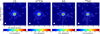 |
Fig. 1. ALMA integrated intensity (moment 0) maps of CS (7–6), H13CN (4–3), SiS (19–18), and 29SiO (8–7) emission lines around W Aql. The ALMA beam (0.55″ × 0.48″, PA 86.35°) is given in the lower-left corner. Contours are marked in white for 1, 3 and 5 σ rms. North is up and east is left. |
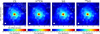 |
Fig. 2. ALMA CO image (color) overlaid with contours (white) of the CS (7–6), H13CN (4–3), SiS (19–18), and 29SiO (8–7) emission, shown at stellar velocity (about −21 km s−1). The ALMA beam for the CS, H13CN, 29SiO and SiS lines (0.55″ × 0.48″, PA 86.35°) is given in the lower-left corner. Contours are plotted for 3, 5, 10 and 20σ rms. North is up and east is left. |
4.1. Morphology of spectral line emission
For the strong spectral line emission – shown in moment-zero maps in Fig. 1 and channel maps in Appendix A – the peak emission seems to be roughly spherical, concentrated at the stellar position, and is spatially resolved. Additionally, we see a fainter and slightly elongated circumstellar emission component extending out to roughly 2–3″. The elongation is oriented in the north-east and south-west (NE/SW) directions, which is also the direction of the binary orbit. We compare the molecular emission of the four strong spectral lines with the CO (3–2) emission reported by Ramstedt et al. (2017) in Fig. 2 and find that the emission features along the NE/SW elongation are equally represented in the CO emission as well, with emission peaks in the molecular lines coinciding with CO emission peaks or clumps.
4.2. Spectral features
The four strongest emission lines (Fig. 3) all show a slight but noticeable excess in blue-shifted emission between approximately −35 and −40 km s−1. This cannot be seen in the channel maps (Appendix A). Additionally, the SiS line shows a strong asymmetry with an excess in red shifted emission relative to the stellar rest frame at around −21 km s−1. This feature can possibly be seen also in the channel maps (Fig. A.3), where between roughly −20 and −14 km s−1 an elongation of the bright peak emission to the east can be seen. It is most prominent at about −16 km s−1, which coincides with the peak of the asymmetry in the spectrum. Furthermore, the 29SiO profile shows two secondary features at about −32 km s−1 and −11 km s−1.
 |
Fig. 3. Spectra of the four strongest spectral lines – CS, H13CN, SiS and 29SiO – measured within a circular 5″ aperture centered on the star. The stellar velocity is at about −21 km s−1. |
Previous models on multiple spectral lines by Danilovich et al. (2014) report a stellar velocity (extracted from the line center velocity), vlsr, of −23 km s−1, which is backed up by and consistent with several other studies, reporting a very similar velocity (e.g., Bieging et al. 1998; Ramstedt et al. 2009; De Beck et al. 2010; Mayer et al. 2013; De Nutte et al. 2017). We note that, investigated separately from previously detected lines, the reported lines observed with ALMA seem to be generally redshifted to this stellar velocity, and a vlsr of −21 km s−1 (such as that calculated by Mayer et al. 2013) is more fitting. Taking the ALMA line peak velocities of all observed lines and calculating an average line peak velocity, we also arrive at a vlsr of −21 km s−1, but the asymmetry of the lines and deviation from parabolic line profiles is very linespecific (as seen in Fig. 3).
4.3. uv fitting
Since the imaging process of interferometric data involves initial knowledge of the source geometry and image artefacts are inevitably introduced during deconvolution, it is reasonable to analyze the observations already in the uv plane, directly working with the calibrated visibility data. For this reason, we use the CASA tool uvmultifit (Martí-Vidal et al. 2014), to fit geometric flux models to the bright emission regions of all spectral lines. Since the TP data combination for this project is done in the image plane and not in the uv plane, we can only fit to the combined 12 m main array and ACA data. This is a reasonable approach, since the maximum recoverable scale for the used 12 m main array and ACA configuration is 19″, and we concentrate our analysis on the central few arcseconds.
Therefore we conclude that for the analysis of the compact, bright emission it is sufficient to use only the main array and ACA data. As a first step, we fit a compact, circular Gaussian component to the data, which is described by its position (relative to the current stellar position of RA 19:15:23.379 and DEC–07:02:50.38 J2000.0 Ramstedt et al. 2017), flux density, and FWHM size. After subtracting the model visibilities from the observed ones, we imaged the residuals to verify the goodness of the Gaussian fit. The resulting residual images for the four strong spectral lines are shown in the top row of Fig. 4. Apart from relatively faint, extended emission surrounding the subtracted compact Gaussian, which can be seen for all four spectral lines, a very compact emission peak remains at the stellar position, which can best be seen in the residual CS and H13CN emission. We succeed in fitting the compact, central emission by adding a delta function to the circular Gaussian, and arrive at significantly better residual images (see Fig. 4, bottom). Figure 5 shows the uv-fitting parameter results for the Gaussian position offset, the Gaussian flux density, and Gaussian FWHM fit parameters, as well as the flux ratio between the added delta component and the Gaussian, for the four strong spectral lines.
 |
Fig. 4. Imaged residuals of the four strong emission lines after subtraction of the model visibilities of a uv fit. Only the central channel at −21 km s−1 is shown. Top row: residuals after the subtraction of the uv fit of a circular Gaussian; bottom row: residuals after the subtraction of the uv fit of a circular Gaussian and a delta function. |
We note, however, that the true intensity distribution of a uniformly expanding envelope is not strictly Gaussian. When the emission is optically thin, the intensity distribution ∝ r−1, which cannot be straightforwardly implemented for use in a uv analysis. When the emission becomes optically thick, the inner part of the distribution flattens, improving a Gaussian approximation. The distribution in the outer envelope can be adequately described using a Gaussian distribution and the deviation mainly becomes apparent in the inner region, close to the resolution limit of our observations. The deviations in this part explain the better fits obtained when including a delta-function, and the strength of the delta function depends on the line optical depth.
The offset of the fitted Gaussian position to the stellar position is well below the spatial resolution of the images and a clear general trend of the offsets for all four lines is barely visible. We note, however, that the photocenter seems to shift with increasing flux density towards slightly larger RA and DEC.
For all four lines, the FWHM size for channels with velocities larger than 0 km s−1 shows very large error bars, meaning that the fit does not converge in those channels and the estimated size of the emission region is very uncertain. The flux density fits show very similar line profiles to the observed ones (a direct comparison is given in Sect. 4.4), with the exception of the 29SiO line profile, which does not show the additional peaks at blue- and red-shifted velocities in the Gaussian fit. The CS, H13CN and 29SiO lines each show a peak in the emission size at blue velocities, which cannot be directly associated with any features in the flux density profile. The only similarity to note here is that the size of the emission region changes at the velocities that belong to the slightly asymmetric and weaker part of the flux density profile. On the other hand, the asymmetric feature in the SiS line profile is associated with a slight increase in emission size. A very similar asymmetry in the SiS line has been observed for the carbon star RW LMi (Lindqvist et al. 2000).
We note that the fitted FWHM of the SiS line lies very close to the imaging resolution at some velocities, meaning that the uv fit is close to over-resolving the emission. We refer to Appendix C for a discussion about super-resolution in uv fitting, as well as the uncertainties attached to the fits.
As expected, the uv-fitting of the four weaker spectral lines is more uncertain and especially for the extreme velocity channels the emission size cannot be constrained confidently. The SiO v = 1 and 30SiS lines seem to be slightly resolved, while the SiO v = 2 and SiS v = 1 lines are unresolved in the image plane, and the signal-to-noise ratio (S/N) for all weak lines is too low for confident fitting. Therefore we refrain from presenting inaccurate uv-fitting results for the weak spectral lines.
4.4. Comparison between uv-fitted and observed spectral shape
We compare the uv-fitted spectra with the observed spectra extracted from the beam convolved images with an aperture of 5″ diameter to compare the spectral contribution of the compact Gaussian and delta function emission components with the fainter, extended asymmetric emission component seen in the residual images (Fig. 4). Figure 6 shows the compared spectra for the strong lines. To illustrate the flux contribution of the compact delta component, we separately show the spectrum of a uv fit with just a circular Gaussian and a spectrum of the uv fit with a circular Gaussian and added delta function component.
 |
Fig. 5. Uv-fitting of the four strong spectral lines detected in the inner CSE of W Aql. First row: RA offset position of the fitted Gaussian. Second row: DEC offset position. Third row: fitted flux-density of circular Gaussian for each velocity bin of 2 km s−1. Fourth row: size of best-fitting circular Gaussian (FWHM). Fifth row: flux ratio of fitted delta function to Gaussian. For reference, the effective beam size in the observed images of 0.55″ × 0.48″ is indicated by a gray dashed line in the fourth row. The gray dashed lines in the two top rows denote the zero point of position offset in RA and DEC, respectively. |
 |
Fig. 6. Comparison of the observed spectra (black) with the uv-fitted spectra of the Gaussian fit (gray) and the fit including a Gaussian plus a delta function (red). The observed spectra were extracted from the images with an aperture of 5″ diameter. The effective beam size in the observed images is 0.55″ × 0.48″. We note that the y-axis scales differently for the first spectral line, which is the strongest. The respective scales are given on the left-hand side for the first line, and on the right-hand side for the remaining lines. |
For all four lines, we see that the fraction of recovered flux is significantly lower when no delta component is added to the uv fit. The model including a Gaussian and a delta component recovers almost the total flux for the CS and H13CN lines, and the majority of flux for the SiS and 29SiO lines. While for CS and H13CN the contribution of the delta component seems to be roughly of the same strength for all velocities, the contribution of the delta component compared to the Gaussian is slightly higher at blue shifted velocities for SiS and 29SiO.
We conclude that the overall emission line profile can be recovered well by uv models of a Gaussian and a delta component, while the remaining small deviations can be attributed to the residual extended and asymmetric emission.
5. Radiative transfer modeling
5.1. Modeling procedure
To model the molecular emission, we used ALI, an accelerated lambda iteration code (first introduced, and later applied and improved by Rybicki & Hummer 1991; Maercker et al. 2008, respectively), following the same procedure as described in Danilovich et al. (2014). The stellar parameters used for the models are given in Table 2. To constrain our models, we used the azimuthally averaged radial profile from the ALMA observations (convolved with a 0.6″ beam) and the ALMA line profiles convolved with a 4″ beam, and additional archival single-dish data listed in Table D.1. We note that the models are primarily fitted to the ALMA data, with the integrated flux of the archival single-dish data being used – in most cases – to discriminate between two equally good fits to the ALMA data. Our model uses the CO modeling results obtained by Danilovich et al. (2014) and refined by Ramstedt et al. (2017). For a distance of 395 pc, 1″ corresponds to 5.91 × 1015 cm or 1 × 1015 cm corresponds to 0.17″.
In all cases, we assumed a Gaussian profile for the molecular fractional abundance distribution, centred on the star, following
 (1)
(1)
where f0 is the abundance relative to H2 at the inner radius of the molecular CSE and Re is the e-folding radius, the radius at which the abundance has dropped off by 1e − 1.
The Gaussian models have two free parameters per molecular species: f0, the central fractional abundance, and Re, the e-folding radius. When considering the ALMA radial profiles, we constrain our models using the central position and offset positions with spacings of 0.1″ starting at 0.05″ and extending to 0.75″, although we include plots showing the models and ALMA profiles out to 2.55″. The error bars on the ALMA observations are derived from an azimuthal average over the observed radial profile. Regarding optical depth, we note that 30SiS and 29SiO are optically thin, CS and 28SiS are mostly optically thin, with the exception of the very innermost regions of CSEs, 28SiO is mostly optically thick, H12CN is very optically thick, and H13CN is optically thick in the shell, but optically thin elsewhere.
Stellar parameters used for radiative transfer modeling.
5.2. Modeling results
When modeling the ALMA radial profiles, we found that for most molecules there was a “tail” in the radial profile, from around 1″ outwards, which could not be fit with a Gaussian abundance profile in a smoothly accelerating CSE model. We first attempted to find a good fit with a non-Gaussian abundance profile, but such models that fit the observations well were not physically realistic, with increasing abundances with radius. Instead, we found that adjusting the wind density over a small region, as could be caused by a binary induced, spiral-like overdensity, for example, greatly improved our model fits to the entire profile. For a smoothly accelerating wind with no overdensities, the H2 number density at radius r is given by
 (2)
(2)
where Ṁ is the mass-loss rate, mH2 is the mass of H2 and υ(r) is the radial velocity profile. To adjust the H2 number density, we multiplied a section of the smooth-wind radial profile (given by the mass-loss rate determined by Ramstedt et al. 2017, listed in Table 2, and the velocity profile defined by Danilovich et al. 2014) by integer factors up to 10. The result that did not overpredict the “tail” for any molecule was chosen as the best model. We found that the inner regions of the radial intensity profiles were not significantly affected by the inclusion of this overdensity and the central abundances and e-folding radii did not need to be adjusted when adding the overdensity.
The best fit for all molecules was found for an overdensity of a factor of five between 8 × 1015 cm and 1.5 × 1016 cm. This reproduces the observed radial profiles for H13CN and 29SiO well, without adjustments to the abundance profiles determined from the smooth-wind models. For SiS and CS, we find that the overdensity model improves the fit to the tail, but not sufficiently to reproduce it entirely. The H2 number densities for both the smooth wind and overdensity models are plotted in Fig. 7. While testing our models, we found that an overdensity factor of ten for SiS or eight for CS were better fits, but these overdensity models strongly over-predicted the H13CN and 29SiO “tails”. Instead, to find the best fits for SiS and CS, we additionally altered their abundances in the overdense region. The scaling factors of the altered abundances are listed in the last column of Table 3. We find this approach justified because the same wind overdensity must be applied to all modeled molecules.
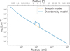 |
Fig. 7. Radial H2 number density for both the smooth wind model and the overdensity model. |
In Table 3, we list the best fit models for both the smooth wind model and the overdensity model, based on the vibrational ground state observations of the respective molecules. The presence of the tail and our overdensity model solution complicates the error analysis of the envelope size. However, if we exclude the overdensity model and discuss only the smooth model, we find that the constraints on the envelope size are tighter for the molecules with less prominent tails and less so for the molecules with the most pronounced tails, such as H13CN. In fact, we found that it was not possible to fit the tail of H13CN simply by increasing the Gaussian e-folding radius, while also providing a good fit to the inner radial points. A Gaussian with a comparable size to the CO envelope (unrealistic in the case of H13CN) would still not fit the tail. Hence the need for the overdensity model.
A comparison of the radial abundance distributions between all modeled molecules as well as some from the earlier study by Danilovich et al. (2014) is presented in Fig. 8. Similarly, in Fig. 9 we plot the best fitting smooth wind and overdensity models against the observed azimuthally averaged radial profiles. There, it is clearly seen that the addition of the overdensity has the most significant impact on the radial profiles of CS and H13CN, giving much better fits to the observations from ~1″ outwards. Below, we discuss the modeling results for the individual spectral lines. In general, the ALMA observations are reasonably well described by the models when looking at the radial intensity profiles, as are the single-dish observations.
 |
Fig. 8. Radial abundance profile. Full lines: molecules observed and modeled in this study, using the overdensity model. Where the abundances differ from the best fitting smooth model, the smooth model is indicated by a dotted line of the same color. Dashed lines: molecules modeled by Danilovich et al. (2014). |
 |
Fig. 9. Radial intensity profiles for the ALMA observations of CS, SiS, 30SiS, 29SiO and H13CN (red circles and dashed lines) compared to the best fitting radiative transfer model with an overdensity (blue squares and solid lines), and the best fitting smooth-wind radiative transfer model (black triangles and dotted lines). |
Results of radiative transfer modeling.
5.2.1. CS
For the radiative transfer analysis of CS, we used a molecular data file including the ground- and first excited vibrational state with rotational energy levels from J = 0 up to J = 40, and their corresponding radiative transitions. Our models include the 8 μm CS vibrational band. The energy levels, transition frequencies, and Einstein A coefficients were taken from CDMS (Müller et al. 2001, 2005) and the collisional rates were adapted from the Yang et al. (2010) rates for CO with H2, assuming an H2 ortho-to-para ratio of three and scaled to represent collisions between CS and H2.
For the smooth wind model, we found a fractional abundance for CS of f0 = 1.20 × 10⁻⁶ and an e-folding radius Re = 7.0 × 1015 cm. While this model fits the inner radial profile and the single dish data well, the outer tail was not well-described by this model. For the overdensity model, using the same Gaussian abundance parameters, we found a much-improved fit, which was improved further by increasing the molecular abundance in the overdense region by a factor of two relative to the Gaussian abundance. The line profile and spectra predicted by the best-fitting (overdensity) model are plotted in Figs. 9 and 10, respectively.
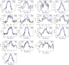 |
Fig. 10. Spectra of different molecular transitions of CS, SiS, 30SiS, 29SiO and H13CN (black histograms) compared to the best fitting radiative transfer model (blue solid lines). |
5.2.2. SiS
For the radiative transfer analysis of 28SiS, we used a molecular data file including the rotational levels from J = 0 up to J = 40 for the ground- and first excited vibrational states, and their corresponding radiative transitions. Our models include the 13 μm SiS vibrational band. The energy levels, transition frequencies and Einstein A coefficients were taken from CDMS (Müller et al. 2001, 2005) and the collisional rates were taken from the Dayou & Balança (2006) rates for SiO with He, scaled to represent collisions between SiS and H2.
For the smooth wind model, we found a fractional abundance for 28SiS of f0 = 1.50 × 10⁻⁶ and an e-folding radius Re = 6.0 × 1015 cm. This model agreed with the single-dish observations well, but did not fully agree with the “tail” in the azimuthally averaged radial profile from the ALMA observations. We found the model improved with the inclusion of the overdensity and, as with CS, an increase of abundance in the overdense region. However, we found that the overdensity and especially the increase of abundance in the overdense region, had a significant effect on the low-J SiS lines, in a way that was not seen for the low-J CS lines at similar (or lower) energies. This provided an additional constraint on the extent of the overdense region, which we were unable to constrain based solely on the ALMA data, and on the abundance increase in the overdense region. An increase in abundance by a factor of seven in the overdense region provides the best fit when considering only the ALMA observations, but strongly over-predicts the single dish (5 → 4) and (12 → 11) SiS lines. Reducing the overdensity abundance down to a factor of three above the smooth wind Gaussian abundance provides the best possible fit when taking both the ALMA radial profile and the single dish observations into account. The line profile and spectra predicted by the best-fit model are plotted in Figs. 9 and 10, respectively.
For the radiative transfer analysis of 30SiS, we constructed the molecular data file to contain the equivalent energy levels and transitions as the 28SiS file.
The energy levels, transition frequencies and Einstein A coefficients were taken from the JPL molecular spectroscopy database (Pickett et al. 1998) and the same collisional rates as for 28SiS were used, based on rates calculated in Dayou & Balança (2006).
We found a fractional abundance for 30SiS of f0 = 1.15 × 10⁻⁷ and an e-folding radius Re = 3.5 × 1015 cm, which is in general agreement with the Re found for 28SiS. The inclusion of the overdensitydidnothaveasignificantimpactonthe30SiSmodelfittothe observations, most likely because the 30SiS flux is much weaker, especially in the region where the brighter molecules exhibit a “tail”. As such, we also had no need to increase the 30SiS abundance in the overdense region. In fact, since the 30SiS flux is weak compared to the 28SiS emission at the location of the employed overdensity, testing the 28SiS overdensity and increased overdensity abundance does not produce a visible change in the 30SiS model.
The line profile and spectra predicted by the 30SiS best-fit model are plotted in Figs. 9 and 10. We include a plot of the spectrum at the center of the source convolved with a 0.6″ beam, in addition to the 4″ beam (used for the other molecules), since the 0.6″ beam spectrum has a significantly higher S/N.
5.2.3. 29SiO
We used the same molecular data file as that used for 29SiO radiative transfer modeling in Danilovich et al. (2014). This includes the rotational energy levels from J = 0 up to J = 40 for the ground and first excited vibrational states. Our models include the 8 μm SiO vibrational band. The collisional rates were also taken from Dayou & Balança (2006).
For the smooth wind model, we found a fractional abundance of 29SiO of f0 = 2.50 × 10⁻⁷ and an e-folding radius Re = 1.4 × 1016 cm. The overdensity model provided a better fit to the azimuthally averaged ALMA radial profile, and did not require an additional adjustment to the abundance profile to reproduce the observations. The line profile and spectra predicted by the best-fit model are plotted in Figs. 9 and 10, respectively.
Our derived 29SiO e-folding radius is in reasonable agreement with the Re for the 28SiO model by Danilovich et al. (2014), indicating that 28SiO and 29SiO are co-spatially distributed in the CSE. As an additional test, we re-ran the 28SiO model using the Re found for 29SiO (and the original f0 = 2.9 × 10⁻⁶ from Danilovich et al. 2014) and found that the smooth wind model was still in good agreement with the single dish 28SiO data, albeit that the low-J single dish data was somewhat over-predicted by the overdensity model.
5.2.4. H13CN
We used the same molecular data file as used for H13CN radiative transfer modeling in Danilovich et al. (2014). This included the rotational energy levels from J = 0 up to J = 29 for the ground vibrational state, the CH stretching mode at 3 μm, and the bending mode at 14 μm. The bending mode is further divided into the two l-type doubling states. The collisional rates were taken from Dumouchel et al. (2010).
For the smooth wind model, we found a fractional abundance for H13CN of f0 = 1.75 × 10⁻⁷ and an e-folding radius Re = 4.7 × 1015 cm. H13CN was one of the molecules for which the overdensity model made the most significant improvement to the fit of the model. No additional increase in abundance was required in the overdense region to reproduce the ALMA data. We also re-ran the H12CN model from Danilovich et al. (2014) with our H13CN Re and the original abundance, f0 = 3.1 × 10⁻⁶, and found that the overdense model still reproduced the (1 → 0) line well. The H13CN line profile and spectra are plotted against the model in Figs. 9 and 10, respectively.
6. Discussion
6.1. Comparison with previous studies
With the ALMA observations at hand, the radial emission size for each measured molecular transition can be extracted directly from the observations and provides an important constraint on the radiative transfer models, which usually use empirical scaling relations to approximate the e-folding radii of individual molecules. Additionally, the sensitivity of interferometric observations is superior to single-dish observations, improving the detection threshold and S/N of the observed spectral lines significantly. This also allowed us to determine a model with an overdense region to better represent the ALMA observations – a feature which cannot be discerned from spatially unresolved observations.
Danilovich et al. (2014) modeled several molecules observed in the CSE of W Aql with multiple lines available. For 29SiO and H13CN, they only have one available line each and assume the same e-folding radii as for the respective main isotopologs. We compare the e-folding radius Re for 29SiO and H13CN measured by this study to the calculated Re by Danilovich et al.(2014), whouse the scaling relations by González Delgado et al. (2003; for 29SiO, assuming the same radial distribution as for 28SiO) and Schöier et al. (2013; for H13CN, assuming the same radial distribution as for H12CN) to estimate the e-folding radius. For 29SiO, the results roughly agree with each other, where we get a radius of 1.4 × 1016 cm and Danilovich et al. (2014) derive a radius of 1.0 × 1016 cm. The same is true for the 29SiO abundance, which Danilovich et al. (2014) find to be (2.3 ± 0.6) × 10−7, which is in agreement within the errors to our derived abundance of (2.50 ± 0.1) × 10−7. For H13CN, we get a radius of 4.7 × 1016 cm, while Danilovich et al. (2014) base their model on a radius of 1.8 × 1016 cm. Our H13CN radius is a factor of approximately three larger than their calculated one. Additionally, we tested the H12CN model from Danilovich et al. (2014; using an abundance of f0 = 3.1 × 10⁻⁶) with the Re for H13CN extracted from this study. We found that that model remained in good agreement with both the higher-J lines, such as (13→12), and the low-J lines, including (1 → 0). The H13CN abundance derived by Danilovich et al. (2014) is (2.8 ± 0.8) × 10−7, which is slightly higher than our result of (1.75 ± 0.05) × 10−7. Since the model from Danilovich et al. (2014) was based only on one single line that showed a particularly pronounced blue wing excess and the fit was based on the integrated intensity, we expect that this discrepancy is caused by the uncertainty of the single-dish observations.
Schöier et al. (2007) present observations and detailed radiative transfer modeling of SiS for a sample of M-type and carbon AGB stars with varying C/O ratios (no S-type stars included), and assume that the SiS radius would be the same as for SiO, and therefore using the scaling relation of González Delgado et al. (2003) to calculate the e-folding radius. With this in mind, we compare the calculated SiO radius of 1.0 × 1016 cm by Danilovich et al. (2014) with our derived SiS radius of 6.0 × 1015 cm, which is a factor of 1.7 smaller. Additionally, Schöier et al. (2007) needed to add a compact, highly abundant SiS component close to the star to better fit their models, which we do not require. Indeed our Gaussian abundance distribution fits both the ALMA and single-dish data well, with the overdensity model only required to fit the outer regions of the ALMA radial profile.
Decin et al. (2008) perform a critical density analysis for SiO, HCN, and CS, which they detect through single-dish observations of a sample of AGB stars – including W Aql – to determine the formation region of the molecular lines. They use two different methods to derive the maximum radius of the emission region (in contrast to the e-folding radius): radiative transfer modeling with the GASTRoNOoM code (Decin et al. 2006) for collisional excitation, and calculations for radiative excitation only. For CS, they derive 1.68 × 1015 cm and 2.64 × 1014 cm, respectively, using a distance of 230 pc (with a luminosity of 6800 L⊙ and an effective temperature of 2800 K). We derive 7.0 × 1015 cm, which is a factor of 4 and 27 larger than their reported values. The different stellar parameters and model setup make it difficult to compare the resulting radii of the emission regions, extracted from different models. As a rough estimate, we scale the reported sizes linearly with the distance and arrive at the conclusion that our CS radius is still bigger than the radii reported by Decin et al. (2008). Comparing their HCN radii – 9.6 × 1014 cm and 2.4 × 1014 cm – to our measured H13CN radius of 4.7 × 1016 cm, we get a substantially larger radius, which also holds for the linear distance scaling. The same is true for the comparison of their SiO radii – 9.6 × 1014 cm and 2.16 × 1014 cm – to our measured 29SiO radius of 1.4 × 1016 cm.
6.2. Limitations of radiative transfer models
The most obvious limitation of the radiative transfer models is that they assume spherical symmetry, which, as we can see from the extended emission in the channel maps, is clearly not a precise description of the more complex emission. This issue becomes more important for the strongest spectral lines, those of CS and H13CN, where the asymmetric features are more pronounced in the observations. For those lines, we see a clear difference between the smooth wind models and the observed radial intensity profiles at distances greater than 1″ from the star (Fig. 9). This is also visible in a much weaker form for the SiS and 29SiO lines (also Fig. 9). Nevertheless, Ramstedt et al. (2017) show that the clearly visible and pronounced arc structures in the CO density distribution are not very pronounced in the overall radial density profile, but are simply represented by rather weak features on top of a smooth extended component. Here, in our overdensity model, we add a higher-density component to the smooth wind model (see Fig. 7) in a region that matches the ALMA radial profiles. Although the actual overdense region is unlikely to be spherically symmetric in reality (as the arcs seen in the CO emission by Ramstedt et al. 2017, are not), we find it to be well fit by our spherically symmetric model.
Another limitation is the direct comparison of often noisy and low-resolution single-dish spectra (often subject to uncertain calibration) with high S/N and high-resolution ALMA spectra as model input. The CS single-dish data in particular generally has a low S/N, and two of the single-dish spectra are not well fitted (Fig. 10). Since the single-dish data were taken at many different epochs, the stellar variability might have an influence on the extracted spectra as well (e.g., Teyssier et al. 2015; Cernicharo et al. 2014) Additionally, since we are probing high-spatial-resolution asymmetric and clumpy emission with the ALMA observations, the line profiles from the symmetric radiative transfer models are unlikely to be completely representative of the real complexity of the CSE around W Aql and therefore do not fit the observations perfectly. Nevertheless, the general agreement of the models with observations is good.
6.3. Comparison with chemical models
From the theoretical models of Cherchneff (2006) and a sample of observations by Bujarrabal & Cernicharo (1994) and Schöier et al. (2007), it is evident that the SiS abundance is sensitive to the chemical type of AGB stars, with carbon stars showing generally higher abundances than M-type stars. The mean fractional SiS abundances of carbon and M-type stars reported by Schöier et al. (2007) are 3.1 × 10⁻⁶ and 2.7 × 10⁻⁷, respectively. Our derived SiS abundance of 1.5 × 10⁻⁶ for W Aql as an S-type star falls close to the lower boundary of the expected region of carbon AGB stars (compared with Fig. 2 of Schöier et al. 2007). Predicted by the non-LTE chemical models of Cherchneff (2006), CS should be found in high abundance for all types of AGB stars in the inner wind, with a generally higher abundance of CS for carbon stars than M-type stars. The formation of CS is linked to HCN, which is predicted to be present in comparable abundances. As discussed by Cherchneff (2006), in their models, the maximum abundance of HCN – and therefore CS – is reached for S-type AGB stars. In Fig. 8, one can see that, for W Aql, the radial abundance profile of HCN (as derived by Danilovich et al. 2014) is indeed comparable to the profile of CS (excluding the overdensity enhancement), which is generally of slightly lower abundance and extends out to a slightly smaller radius. The abundance ratio of those molecules is HCN/CS = 3.1 × 10⁻⁶/1.3 × 10−6 ≃ 2.4. In the theoretical models of Cherchneff (2006), the HCN/CS ratio for a “typical” AGB with a C/O ratio between 0.75 and 1 lies between 5.34 and 0.28, at radii larger than 5 R⋆. The best fitting theoretical HCN/CS ratio to our modeled ratio of 2.4 would be reached for a C/O ratio somewhere between 0.90 and 0.98. The theoretical HCN/CS ratio of 0.28 for a C/O ratio of 1 does not fit our models. A very similar value can be derived from thermodynamic equilibrium calculations (Gobrecht, priv. comm.), which yield a HCN abundance of 4.31 × 10⁻⁸ and a CS abundance of 1.38 × 10⁻⁷, resulting in a HCN/CS ratio of 0.31. It must be noted, however, that the chemical models are focused on the innermost winds and our observations detect molecular emission as far away from the star as ~4″. Additionally, the stellar temperature can affect the chemical equilibrium and therefore the chemical abundances.
On a general note on sulphur bearing molecules in CSEs of AGB stars, Danilovich et al. (2016) found a very different S chemistry between low mass-loss rate and high mass-loss rate M-type stars when examining SO and SO2, which was not predicted by chemical models.
6.4. Isotopic ratios
6.4.1. Silicon
Previous models by Danilovich et al. (2014) estimate a 28SiO abundance of 2.9 × 10⁻⁶, which we can use to derive the 28SiO/29SiO ratio, resulting in a value of 11.6. From our model estimates, we find the abundance ratio of 28SiS/30SiS = 13.0, roughly corresponding to half of the 28Si/30Si ratio predicted by AGB stellar evolution models (Cristallo et al. 2015; Karakas 2010) and half of the value given by the solar abundances (Asplund et al. 2009). By assuming that both SiO and SiS ratios are good tracers for the Si ratios, we can approximate the 29Si/30Si ratio for W Aql, which results in a value of 1.1. For comparison, the solar 29Si/30Si ratio, as derived by Asplund et al. (2009) is 1.52, which is also consistent with the ratio derived for the ISM (Wolff 1980; Penzias 1981). Peng et al. (2013) investigate the 29Si/30Si ratio for 15 evolved stars and come to the conclusion that the older low-mass oxygen-rich stars in their sample have lower 29Si/30Si ratios, but the ratios are not influenced strongly by AGB evolution and merely reflect the interstellar environment in which the star has been born. The only S-type star in their sample, χ Cyg, shows a 29Si/30Si ratio of 1.1, which is incidentally identical to our derived value for W Aql. A bigger sample of Si isotopic ratios derived for S-type stars would be needed to draw any conclusions on the possible AGB evolutionary effects.
6.4.2. Carbon
As described by Saberi et al. (2017) for the carbon AGB star R Scl, the H12CN/H13CN ratio is a very good tracer for the 12C/13C ratio, giving even more plausible results than estimates from the CO isotopic ratio in some cases. Using modeling results by Danilovich et al. (2014) for H12CN, which has an abundance of (3.1 ± 0.1) × 10−6, and the H13CN abundance presented in this paper, we derive a H12CN/H13CN ratio of 17 ± 6 (with the error mainly dominated by the H12CN model), which can be used to estimate the 12C/13C ratio. This result differs by a factor of 1.7 to 1.5 from the 12C/13C ratio estimated from the CO isotopolog ratio by Danilovich et al. (2014) and Ramstedt & Olofsson (2014), who report a ratio of 29 and 26, respectively. Ramstedt & Olofsson (2014) also present C isotopic ratios for 16 other S-type AGB stars (in addition to 19 C- and 19 M-type AGB stars) and the resulting median carbon isotopic ratio for S-type stars is reported to be 26, which is also their derived value for W Aql. In general, the 12C/13C ratio increases following the evolution from M- to S- to C-type stars, since 12C is primarily produced in the He burning shell of the star and will be dredged up to the surface through subsequent thermal pulses. Therefore, the 12C/13C ratio can be used as an indicator for the AGB evolutionary stage of a star.
7. Conclusions
We present ALMA observations of a total of eight molecular lines of the species CS, SiS, SiO and H13CN, which are found in the close CSE of the S-type binary AGB star W Aql. The emission is resolved for almost all lines and a compact Gaussian emission component is surrounded by weak asymmetric emission, showing an elongation in the direction of the binary orbit. Adding an additional delta function emission component to the models at the same position as the Gaussian significantly improves the fits, carried out in the uv plane. Emission peaks in molecular emission out to approximately 2–3″ coincide with the CO distribution. The spectral lines – especially the strongest four – are partly very asymmetric, with SiS standing out of the sample with a very distinct peak at the red-shifted velocities. We successfully model the circumstellar abundance and radial emission size of CS, SiS, 30SiS, 29SiO and H13CN – mainly based on high-resolution sub-millimeter observations by ALMA and supplemented by archival single-dish observations – in the innermost few arcseconds of the CSE around the S-type AGB star W Aql. We produce two models, one assuming a smooth outflow, and one which approximates the asymmetries seen in the outflow by the inclusion of an overdense component, and which better fits the ALMA data. We compare the resultant radial abundance distributions to previous modeling and theoretical predictions, and find that our results are in agreement with previous studies. For some isotopologs, such as 29SiO and H13CN, previous studies worked with the assumption of a radial distribution identical to their main isotopologs, 28SiO and H12CN. We find that our modeled radial distribution of the 29SiO and H13CN isotopologs, which is constrained by the resolved ALMA observations, is different to the main isotopologs, with both rarer isotopologs having a larger radius than previously found for the most common isotopolog counterparts.
By using the spatially resolved ALMA data, we can constrain the radial emission profile directly, which improves the independence of our models by reducing the number of input assumptions. Additionally, we need to develop improved models, which can take asymmetries into account. This and future high-resolution high sensitivity spectral scans of CSEs around AGB stars will provide more accurate input to chemical modeling and help us understand the chemical network of elements in these environments.
Acknowledgments
This paper makes use of the following ALMA data: ADS/JAO.ALMA#2012.1.00524.S. ALMA is a partnership of ESO (representing its member states), NSF (USA) and NINS (Japan), together with NRC (Canada), NSC and ASIAA (Taiwan), and KASI (Republic of Korea), in cooperation with the Republic of Chile. The Joint ALMA Observatory is operated by ESO, AUI/NRAO and NAOJ. We want to thank the Nordic ARC Node for valuable support concerning ALMA data reduction and uv-fitting, and David Gobrecht for his input to the chemical discussion. MB acknowledges the support by the uni:docs fellowship and the dissertation completion fellowship of the University of Vienna. EDB is supported by the Swedish National Space Board. TD acknowledges support from the Fund of Scientific Research Flanders (FWO).
References
- Asplund, M., Grevesse, N., Sauval, A. J., & Scott, P. 2009, ARA&A, 47, 481 [NASA ADS] [CrossRef] [Google Scholar]
- Bieging, J. H., Knee, L. B. G., Latter, W. B., & Olofsson, H. 1998, A&A, 339, 811 [NASA ADS] [Google Scholar]
- Bladh, S., & Höfner, S. 2012, A&A, 546, A76 [NASA ADS] [CrossRef] [EDP Sciences] [Google Scholar]
- Bladh, S., Höfner, S., Aringer, B., & Eriksson, K. 2015, in Why Galaxies Care about AGB Stars III: A Closer Look in Space and Time, eds. F. Kerschbaum, R. F. Wing, & J. Hron, ASP Conf. Ser., 497, 345 [NASA ADS] [Google Scholar]
- Bujarrabal, V., & Cernicharo, J. 1994, A&A, 288, 551 [NASA ADS] [Google Scholar]
- Cernicharo, J., Teyssier, D., Quintana-Lacaci, G., et al. 2014, ApJ, 796, L21 [NASA ADS] [CrossRef] [Google Scholar]
- Cherchneff, I. 2006, A&A, 456, 1001 [NASA ADS] [CrossRef] [EDP Sciences] [Google Scholar]
- Cristallo, S., Straniero, O., Piersanti, L., & Gobrecht, D. 2015, ApJS, 219, 40 [NASA ADS] [CrossRef] [Google Scholar]
- Cutri, R. M., Skrutskie, M. F., van Dyk, S., et al. 2003, VizieR Online Data Catalog, II/246 [Google Scholar]
- Danilovich, T., Bergman, P., Justtanont, K., et al. 2014, A&A, 569, A76 [NASA ADS] [CrossRef] [EDP Sciences] [Google Scholar]
- Danilovich, T., Teyssier, D., Justtanont, K., et al. 2015, A&A, 581, A60 [NASA ADS] [CrossRef] [EDP Sciences] [Google Scholar]
- Danilovich, T., De Beck, E., Black, J. H., Olofsson, H., & Justtanont, K. 2016, A&A, 588, A119 [NASA ADS] [CrossRef] [EDP Sciences] [Google Scholar]
- Danilovich, T., Ramstedt, S., Gobrecht, D., et al. 2018, A&A, in press, DOI: 10.1051/0004-6361/201833317 [Google Scholar]
- Dayou, F., & Balança, C. 2006, A&A, 459, 297 [NASA ADS] [CrossRef] [EDP Sciences] [Google Scholar]
- De Beck, E., Decin, L., de Koter, A., et al. 2010, A&A, 523, A18 [NASA ADS] [CrossRef] [EDP Sciences] [Google Scholar]
- De Nutte, R., Decin, L., Olofsson, H., et al. 2017, A&A, 600, A71 [NASA ADS] [CrossRef] [EDP Sciences] [Google Scholar]
- Decin, L., Hony, S., de Koter, A., et al. 2006, A&A, 456, 549 [NASA ADS] [CrossRef] [EDP Sciences] [Google Scholar]
- Decin, L., Cherchneff, I., Hony, S., et al. 2008, A&A, 480, 431 [Google Scholar]
- Dumouchel, F., Faure, A., & Lique, F. 2010, MNRAS, 406, 2488 [NASA ADS] [CrossRef] [Google Scholar]
- Feast, M. W., & Whitelock, P. A. 2000, MNRAS, 317, 460 [NASA ADS] [CrossRef] [Google Scholar]
- Glass, I. S., & Evans, T. L. 1981, Nature, 291, 303 [NASA ADS] [CrossRef] [Google Scholar]
- González Delgado, D., Olofsson, H., Kerschbaum, F., et al. 2003, A&A, 411, 123 [NASA ADS] [CrossRef] [EDP Sciences] [Google Scholar]
- Groenewegen, M. A. T., Waelkens, C., Barlow, M. J., et al. 2011, A&A, 526, A162 [NASA ADS] [CrossRef] [EDP Sciences] [Google Scholar]
- Habing, H. J., & Olofsson, H., 2003, Asymptotic Giant Branch Stars (New York, Berlin: Springer) [Google Scholar]
- Höfner, S. 2008, A&A, 491, L1 [NASA ADS] [CrossRef] [EDP Sciences] [Google Scholar]
- Höfner, S. 2015, in Why Galaxies Care about AGB Stars III: A Closer Look in Space and Time, eds. F. Kerschbaum, R. F. Wing, & J. Hron, ASP Conf. Ser., 497, 333 [NASA ADS] [Google Scholar]
- Karakas, A. I. 2010, MNRAS, 403, 1413 [NASA ADS] [CrossRef] [Google Scholar]
- Keenan, P. C., & Boeshaar, P. C. 1980, ApJS, 43, 379 [NASA ADS] [CrossRef] [EDP Sciences] [Google Scholar]
- Knapp, G. R., Young, K., Lee, E., & Jorissen, A. 1998, ApJS, 117, 209 [NASA ADS] [CrossRef] [Google Scholar]
- Lindqvist, M., Schöier, F. L., Lucas, R., & Olofsson, H. 2000, A&A, 361, 1036 [NASA ADS] [Google Scholar]
- Maercker, M., Schöier, F. L., Olofsson, H., Bergman, P., & Ramstedt, S. 2008, A&A, 479, 779 [NASA ADS] [CrossRef] [EDP Sciences] [Google Scholar]
- Maercker, M., Vlemmings, W. H. T., Brunner, M., et al. 2016, A&A, 586, A5 [NASA ADS] [CrossRef] [EDP Sciences] [Google Scholar]
- Martí-Vidal, I., Pérez-Torres, M. A., & Lobanov, A. P. 2012, A&A, 541, A135 [NASA ADS] [CrossRef] [EDP Sciences] [Google Scholar]
- Martí-Vidal, I., Vlemmings, W. H. T., Muller, S., & Casey, S. 2014, A&A, 563, A136 [NASA ADS] [CrossRef] [EDP Sciences] [Google Scholar]
- Mayer, A., Jorissen, A., Kerschbaum, F., et al. 2013, A&A, 549, A69 [NASA ADS] [CrossRef] [EDP Sciences] [Google Scholar]
- Menten, K. M., Wyrowski, F., Alcolea, J., et al. 2010, A&A, 521, L7 [NASA ADS] [CrossRef] [EDP Sciences] [Google Scholar]
- Müller, H. S. P., Thorwirth, S., Roth, D. A., & Winnewisser, G. 2001, A&A, 370, L49 [NASA ADS] [CrossRef] [EDP Sciences] [Google Scholar]
- Müller, H. S. P., Schlöder, F., Stutzki, J., & Winnewisser, G. 2005, J. Mol. Struct., 742, 215 [NASA ADS] [CrossRef] [Google Scholar]
- Neufeld, D. A., Gusdorf, A., Güsten, R., et al. 2014, ApJ, 781, 102 [NASA ADS] [CrossRef] [Google Scholar]
- Olofsson, H., González Delgado, D., Kerschbaum, F., & Schöier, F. L. 2002, A&A, 391, 1053 [NASA ADS] [CrossRef] [EDP Sciences] [Google Scholar]
- Patel, N. A., Young, K. H., Gottlieb, C. A., et al. 2011, ApJS, 193, 17 [NASA ADS] [CrossRef] [Google Scholar]
- Peng, T.-C., Humphreys, E. M. L., Testi, L., et al. 2013, A&A, 559, L8 [NASA ADS] [CrossRef] [EDP Sciences] [Google Scholar]
- Penzias, A. A. 1981, ApJ, 249, 513 [NASA ADS] [CrossRef] [Google Scholar]
- Pickett, H. M., Poynter, R. L., Cohen, E. A., et al. 1998, J. Quant. Spectr. Rad. Transf., 60, 883 [NASA ADS] [CrossRef] [Google Scholar]
- Ramstedt, S., & Olofsson, H. 2014, A&A, 566, A145 [NASA ADS] [CrossRef] [EDP Sciences] [Google Scholar]
- Ramstedt, S., Schöier, F. L., & Olofsson, H. 2009, A&A, 499, 515 [NASA ADS] [CrossRef] [EDP Sciences] [Google Scholar]
- Ramstedt, S., Maercker, M., Olofsson, G., Olofsson, H., & Schöier, F. L. 2011, A&A, 531, A148 [NASA ADS] [CrossRef] [EDP Sciences] [Google Scholar]
- Ramstedt, S., Mohamed, S., Vlemmings, W. H. T., et al. 2017, A&A, 605, A126 [NASA ADS] [CrossRef] [EDP Sciences] [Google Scholar]
- Rybicki, G. B., & Hummer, D. G. 1991, A&A, 245, 171 [NASA ADS] [Google Scholar]
- Saberi, M., Maercker, M., De Beck, E., et al. 2017, A&A, 599, A63 [NASA ADS] [CrossRef] [EDP Sciences] [Google Scholar]
- Schmidt, M. R., He, J. H., Szczerba, R., et al. 2016, A&A, 592, A131 [NASA ADS] [CrossRef] [EDP Sciences] [Google Scholar]
- Schöier, F. L., Ryde, N., & Olofsson, H. 2002, A&A, 391, 577 [NASA ADS] [CrossRef] [EDP Sciences] [Google Scholar]
- Schöier, F. L., Bast, J., Olofsson, H., & Lindqvist, M. 2007, A&A, 473, 871 [NASA ADS] [CrossRef] [EDP Sciences] [Google Scholar]
- Schöier, F. L., Ramstedt, S., Olofsson, H., et al. 2013, A&A, 550, A78 [NASA ADS] [CrossRef] [EDP Sciences] [Google Scholar]
- Tatebe, K., Chandler, A. A., Hale, D. D. S., & Townes, C. H. 2006, ApJ, 652, 666 [NASA ADS] [CrossRef] [Google Scholar]
- Teyssier, D., Cernicharo, J., Quintana-Lacaci, G., et al. 2015, in Why Galaxies Care about AGB Stars III: A Closer Look in Space and Time, eds. F. Kerschbaum, R. F. Wing, & J. Hron, ASP Conf. Ser., 497, 43 [Google Scholar]
- Uttenthaler, S. 2013, A&A, 556, A38 [NASA ADS] [CrossRef] [EDP Sciences] [Google Scholar]
- Van Eck, S., Neyskens, P., Jorissen, A., et al. 2017, A&A, 601, A10 [Google Scholar]
- Whitelock, P. A., Feast, M. W., & van Leeuwen, F. 2008, MNRAS, 386, 313 [NASA ADS] [CrossRef] [Google Scholar]
- Wolff, R. S. 1980, ApJ, 242, 1005 [NASA ADS] [CrossRef] [Google Scholar]
- Yang, B., Stancil, P. C., Balakrishnan, N., & Forrey, R. C. 2010, ApJ, 718, 1062 [NASA ADS] [CrossRef] [Google Scholar]
- Zijlstra, A. A., Bedding, T. R., Markwick, A. J., et al. 2004, MNRAS, 352, 325 [NASA ADS] [CrossRef] [Google Scholar]
Appendix A: Channel maps for strong spectral lines
 |
Fig. A.1. Channel map for the CS spectral line. The velocity resolution is 1 km s−1, only every second channel is plotted. The stellar velocity is at about −21 km s−1. The beam size is given in the lower left and the white contours are plotted for 3, 5, and 10 σ rms (measured from line free channels). North is up and east is left. |
 |
Fig. A.2. Channel map for the H13CN spectral line. The velocity resolution is 1 km s−1, only every second channel is plotted. The stellar velocity is at about −21 km s−1. The beam size is given in the lower left and the white contours are plotted for 3, 5, and 10 σ rms (measured from line free channels). North is up and east is left. |
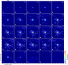 |
Fig. A.3. Channel map for the SiS spectral line. The velocity resolution is 1 km s−1, only every second channel is plotted. The stellar velocity is at about −21 km s−1. The beam size is given in the lower left and the white contours are plotted for 3, 5, and 10 σ rms (measured from line free channels). North is up and east is left. |
 |
Fig. A.4. Channel map for the 29SiO spectral line. The velocity resolution is 1 km s−1, only every second channel is plotted. The stellar velocity is at about −21 km s−1. The beam size is given in the lower left and the white contours are plotted for 3, 5, and 10 σ rms (measured from line free channels). North is up and east is left. |
Appendix B: Results for weak spectral lines
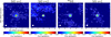 |
Fig. B.1. ALMA integrated intensity (moment 0) maps of SiO v = 1 (8–7), SiO v = 2 (8–7), 30SiS (19–18) and SiS v = 1 (19–18) emission around W Aql. The ALMA beam is given in the lower-left corner. Contours are given in white for 1, 2, and 3 σ rms. North is up and east is left. |
Appendix C: uv-fitting: super-resolution and uncertainties
As has been discussed in Martí-Vidal et al. (2012), high S/N interferometric observations may encode information about source substructures (much) smaller than the diffraction limit of the interferometer. Extracting such information, though, implies the use of a priori assumptions related to the source brightness distribution (e.g., the assumption of a Gaussian intensity distribution that we are using in our modeling). As long as the true source structure obeys these a priori assumptions (at least to the extent of the structure sizes being probed in the visibility analysis), it is possible to retrieve structure information that roughly scales as the diffraction limit divided by the square root of the S/N (see, e.g., Eq. (7) of Martí-Vidal et al. 2012). We notice, though, that this is an approximate rule of thumb that may be corrected by a factor of several, since the actual over-resolution power may depend on the baseline distribution of the array (i.e., the factor β in Eq. (7) of Martí-Vidal et al. 2012).
The modeling performed by uvmultifit (Martí-Vidal et al. 2014) estimates the uncertainties of the fitted parameters from the curvature of the χ2 distribution at its minimum via the diagonal elements of the post-fit covariance matrix. The uncertainties provided in this way assume that the model used in the fit is correct and able to describe the bulk of the visibility signal, meaning that the reduced χ2 can be assumed to be similar to its expected value of unity.
This assumption may result in underestimates of the parameter uncertainties if the model used in the fitting is incorrect. One way to test whether our fitting model is able to describe the bulk of the visibility function is to assess the post-fit residuals in the image plane. We show these residuals for a selection of two channels in the SiS line in Fig. C.1 (left). The intensity distribution of the residuals can be well characterized by Gaussian noise (Fig. C.1, right), which is indicative of a successful fit.
In order to further assess our size estimates and uncertainties, we have performed a Monte Carlo analysis of our Gaussian source model plus additional delta component across the full parameter space (i.e., varying the peak position, flux density, and size with a random exploration), to test how the χ2 (and hence the probability density) varies in the neighborhood of the best-fit parameter values. We show the resulting probability density functions (PDF) for channels 13 and 20 in Fig. C.2. We notice that the standard assumptions of uvmultifit are applied here (i.e., a reduced χ2 of 1 is assumed, which is justified by the post-fit residuals; see Fig. C.1). The crossing points between the 3σ deviations of the source size (vertical dashed lines) and the 3σ probability cutoff for a Gaussian PDF (horizontal dashed line) roughly coincide with the crossing points between the 3σ source-size deviation and the PDF retrieved with uvmultifit.
We can therefore conclude that, as long as the Gaussian plus delta component brightness distribution is a good approximation of the source structure, the source sizes (and their uncertainties) obtained with uvmultifit are correct. If the source shape were to not resemble a Gaussian brightness distribution, but were closer to, say, a disk or a filled sphere, there would be a global systematic bias in all source sizes reported here, even though the relative values among frequency channels (i.e., the frequency dependence of the source sizes) would still be correct.
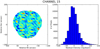 |
Fig. C.1. Left: post-fit residual image for channel 15 (stellar velocity), using natural weighting (i.e., to maximise the detection sensitivity for any flux-density contribution left in the fitting). Right: histogram of the post-fit image residuals. |
 |
Fig. C.2. Probability density distributions from our model-fitting for the SiS line of channels 15 and 20, using a Gaussian source model with addition of a delta function model. The vertical dashed lines indicate the estimated best-fit values and their ±3σ deviations. The horizontal dashed line is set to 3 × 10⁻³ (i.e., the probability density corresponding to the 3σ cutoff of a Gaussian probability distribution). The peaks of the PDFs have been further scaled to 1, for clarity. |
Appendix D: List of archival spectral line observations
Archival observations.
All Tables
All Figures
|
Fig. 1. ALMA integrated intensity (moment 0) maps of CS (7–6), H13CN (4–3), SiS (19–18), and 29SiO (8–7) emission lines around W Aql. The ALMA beam (0.55″ × 0.48″, PA 86.35°) is given in the lower-left corner. Contours are marked in white for 1, 3 and 5 σ rms. North is up and east is left. |
| In the text | |
|
Fig. 2. ALMA CO image (color) overlaid with contours (white) of the CS (7–6), H13CN (4–3), SiS (19–18), and 29SiO (8–7) emission, shown at stellar velocity (about −21 km s−1). The ALMA beam for the CS, H13CN, 29SiO and SiS lines (0.55″ × 0.48″, PA 86.35°) is given in the lower-left corner. Contours are plotted for 3, 5, 10 and 20σ rms. North is up and east is left. |
| In the text | |
|
Fig. 3. Spectra of the four strongest spectral lines – CS, H13CN, SiS and 29SiO – measured within a circular 5″ aperture centered on the star. The stellar velocity is at about −21 km s−1. |
| In the text | |
|
Fig. 4. Imaged residuals of the four strong emission lines after subtraction of the model visibilities of a uv fit. Only the central channel at −21 km s−1 is shown. Top row: residuals after the subtraction of the uv fit of a circular Gaussian; bottom row: residuals after the subtraction of the uv fit of a circular Gaussian and a delta function. |
| In the text | |
|
Fig. 5. Uv-fitting of the four strong spectral lines detected in the inner CSE of W Aql. First row: RA offset position of the fitted Gaussian. Second row: DEC offset position. Third row: fitted flux-density of circular Gaussian for each velocity bin of 2 km s−1. Fourth row: size of best-fitting circular Gaussian (FWHM). Fifth row: flux ratio of fitted delta function to Gaussian. For reference, the effective beam size in the observed images of 0.55″ × 0.48″ is indicated by a gray dashed line in the fourth row. The gray dashed lines in the two top rows denote the zero point of position offset in RA and DEC, respectively. |
| In the text | |
|
Fig. 6. Comparison of the observed spectra (black) with the uv-fitted spectra of the Gaussian fit (gray) and the fit including a Gaussian plus a delta function (red). The observed spectra were extracted from the images with an aperture of 5″ diameter. The effective beam size in the observed images is 0.55″ × 0.48″. We note that the y-axis scales differently for the first spectral line, which is the strongest. The respective scales are given on the left-hand side for the first line, and on the right-hand side for the remaining lines. |
| In the text | |
|
Fig. 7. Radial H2 number density for both the smooth wind model and the overdensity model. |
| In the text | |
|
Fig. 8. Radial abundance profile. Full lines: molecules observed and modeled in this study, using the overdensity model. Where the abundances differ from the best fitting smooth model, the smooth model is indicated by a dotted line of the same color. Dashed lines: molecules modeled by Danilovich et al. (2014). |
| In the text | |
|
Fig. 9. Radial intensity profiles for the ALMA observations of CS, SiS, 30SiS, 29SiO and H13CN (red circles and dashed lines) compared to the best fitting radiative transfer model with an overdensity (blue squares and solid lines), and the best fitting smooth-wind radiative transfer model (black triangles and dotted lines). |
| In the text | |
|
Fig. 10. Spectra of different molecular transitions of CS, SiS, 30SiS, 29SiO and H13CN (black histograms) compared to the best fitting radiative transfer model (blue solid lines). |
| In the text | |
|
Fig. A.1. Channel map for the CS spectral line. The velocity resolution is 1 km s−1, only every second channel is plotted. The stellar velocity is at about −21 km s−1. The beam size is given in the lower left and the white contours are plotted for 3, 5, and 10 σ rms (measured from line free channels). North is up and east is left. |
| In the text | |
|
Fig. A.2. Channel map for the H13CN spectral line. The velocity resolution is 1 km s−1, only every second channel is plotted. The stellar velocity is at about −21 km s−1. The beam size is given in the lower left and the white contours are plotted for 3, 5, and 10 σ rms (measured from line free channels). North is up and east is left. |
| In the text | |
|
Fig. A.3. Channel map for the SiS spectral line. The velocity resolution is 1 km s−1, only every second channel is plotted. The stellar velocity is at about −21 km s−1. The beam size is given in the lower left and the white contours are plotted for 3, 5, and 10 σ rms (measured from line free channels). North is up and east is left. |
| In the text | |
|
Fig. A.4. Channel map for the 29SiO spectral line. The velocity resolution is 1 km s−1, only every second channel is plotted. The stellar velocity is at about −21 km s−1. The beam size is given in the lower left and the white contours are plotted for 3, 5, and 10 σ rms (measured from line free channels). North is up and east is left. |
| In the text | |
|
Fig. B.1. ALMA integrated intensity (moment 0) maps of SiO v = 1 (8–7), SiO v = 2 (8–7), 30SiS (19–18) and SiS v = 1 (19–18) emission around W Aql. The ALMA beam is given in the lower-left corner. Contours are given in white for 1, 2, and 3 σ rms. North is up and east is left. |
| In the text | |
|
Fig. C.1. Left: post-fit residual image for channel 15 (stellar velocity), using natural weighting (i.e., to maximise the detection sensitivity for any flux-density contribution left in the fitting). Right: histogram of the post-fit image residuals. |
| In the text | |
|
Fig. C.2. Probability density distributions from our model-fitting for the SiS line of channels 15 and 20, using a Gaussian source model with addition of a delta function model. The vertical dashed lines indicate the estimated best-fit values and their ±3σ deviations. The horizontal dashed line is set to 3 × 10⁻³ (i.e., the probability density corresponding to the 3σ cutoff of a Gaussian probability distribution). The peaks of the PDFs have been further scaled to 1, for clarity. |
| In the text | |
Current usage metrics show cumulative count of Article Views (full-text article views including HTML views, PDF and ePub downloads, according to the available data) and Abstracts Views on Vision4Press platform.
Data correspond to usage on the plateform after 2015. The current usage metrics is available 48-96 hours after online publication and is updated daily on week days.
Initial download of the metrics may take a while.