| Issue |
A&A
Volume 617, September 2018
|
|
|---|---|---|
| Article Number | A66 | |
| Number of page(s) | 14 | |
| Section | Galactic structure, stellar clusters and populations | |
| DOI | https://doi.org/10.1051/0004-6361/201832670 | |
| Published online | 13 September 2018 | |
The Arches cluster revisited
II. A massive eclipsing spectroscopic binary in the Arches cluster★
1
School of Physical Sciences, The Open University, Walton Hall,
Milton Keynes
MK7 6AA, UK
e-mail: This email address is being protected from spambots. You need JavaScript enabled to view it.
2
Centro de Astrobiología (CSIC-INTA), Ctra. de Torrejón a Ajalvir md-4,
28850
Torrejón de Ardoz,
Madrid, Spain
3
Instituto de Astrofísica de Canarias,
38205
La Laguna,
Tenerife, Spain
4
Departamento de Astrofísica, Universidad de La Laguna,
38206
La Laguna,
Tenerife, Spain
5
Institute for Astronomy, University of Edinburgh, Royal Observatory Edinburgh,
Blackford Hill,
Edinburgh
EH9 3HJ, UK
6
Department of Physics and Astronomy, University of Sheffield,
Sheffield
S3 7RH, UK
7
UK Astronomy Technology Centre, Royal Observatory,
Blackford Hill,
Edinburgh
EH9 3HJ, UK
Received:
19
January
2018
Accepted:
14
April
2018
Abstract
We have carried out a spectroscopic variability survey of some of the most massive stars in the Arches cluster, using K-band observations obtained with SINFONI on the VLT. One target, F2, exhibits substantial changes in radial velocity (RV); in combination with new KMOS and archival SINFONI spectra, its primary component is found to undergo RV variation with a period of 10.483 ± 0.002 d and an amplitude of ~350 km s−1. A secondary RV curve is also marginally detectable. We reanalysed archival NAOS-CONICA photometric survey data in combination with our RV results to confirm this object as an eclipsing SB2 system, and the first binary identified in the Arches. We have modelled it as consisting of an 82 ± 12 M⊙ WN8–9h primary and a 60 ± 8 M⊙ O5–6 Ia+ secondary, and as having a slightly eccentric orbit, implying an evolutionary stage prior to strong binary interaction. As one of four X-ray bright Arches sources previously proposed as colliding-wind massive binaries, it may be only the first of several binaries to be discovered in this cluster, presenting potential challenges to recent models for the Arches’ age and composition. It also appears to be one of the most massive binaries detected to date; the primary’s calculated initial mass of ≳120 M⊙ would arguably make this the most massive binary known in the Galaxy.
Key words: stars: individual: F2 / stars: massive / stars: Wolf–Rayet / binaries: close / binaries: eclipsing / binaries: spectroscopic
The individual reduced spectra and the two disentangled spectra are only available at the CDS via anonymous ftp to cdsarc.u-strasbg.fr (130.79.128.5) or via http://cdsarc.u-strasbg.fr/viz-bin/qcat?J/A+A/617/A66.
© ESO 2018
1 Introduction
The Arches cluster, discovered about 20 years ago (Nagata et al. 1995; Cotera et al. 1996) near the Galactic centre, contains a remarkable, dense population of young, very massive stars. Using K-band spectroscopy, around 200 O and OIf+ supergiants and a dozen WNLh-type Wolf–Rayet stars have been identified (Blum et al. 2001; Figer et al. 2002; Martins et al. 2008), and the total cluster mass is of the order of 104 M⊙ (Stolte et al. 2002). It is thus very valuable for investigations of the formation and evolution of the most massive stars, and even for constraining the upper stellar mass limit (Figer 2005). It is also highly significant for our understanding of star formation near the centre of our Galaxy, along with the Quintuplet cluster and Galactic central cluster itself.
Identifying massive binaries in the Arches would be useful in several ways. Such objects are of intrinsic interest as candidate progenitors for supernovae of various types, gamma-ray bursts and even merging binary stellar mass black holes like GW150914 (Abbott et al. 2016). Moreover, a double-lined spectroscopic and eclipsing binary would permit direct mass determinations for its components, providing a check on masses estimated from model evolutionary tracks. This in turn would have implications for the age of the cluster: Martins et al. (2008) agreed with Figer et al.’s (2002) estimate of 2.5 ± 0.5 Myr, at least for the most massive, luminous stars, but Schneider et al. (2014) have argued that an age of 3.5 ± 0.7 Myr is more plausible, on the basis of fitting their population synthesis models to a stellar mass function for the cluster, with an associated conclusion that the most massive cluster members are rejuvenated products of binary interaction and merger. The detection of existing massive binaries would contribute to the resolution of this debate.
There are already indications of possible colliding-wind binaries in the Arches from radio (Lang et al. 2001, 2005) and X-ray (Wang et al. 2006) observations. A candidate massive contact eclipsing binary was also proposed as a preliminary result of a photometricvariability survey (Markakis et al. 2011). However, the detection of regular radial velocity (RV) variations allows binaries to be confirmed and, in combination with suitable light curves, their masses constrained (e.g. Ritchie et al. 2009, 2010; Clark et al. 2011). Therefore, we have undertaken a multi-epoch spectroscopic survey of the most massive members of the Arches, reported in Clark et al. (2018) and Lohr et al. in prep., hereafter Papers I and III. Here, in Paper II, we describe our detection and investigation of the target which gave the strongest evidence for binarity, and for which sufficient additional data were available to permit preliminary modelling.
2 Data acquisition and reduction
2.1 Spectroscopy
This section focuses upon the observations and data reduction specific to the binary which is the subject of this paper. For full details of the reduction procedures used and the nature of the wider spectroscopic survey, see Paper I.
The SINFONI integral field spectrograph on the ESO/VLT (Eisenhauer et al. 2003; Bonnet et al. 2004) was used in service mode to observe fields in the central Arches cluster, and on the periphery of the cluster, in the K band, during April – August 2011, and March – August 20131. The data cubes were reduced, and the stellar spectra extracted, as described in Paper I. Objects were observed on up to seven distinct epochs; the main subject of this paper, F2 (i.e. the second object on the list of Figer et al. 2002) was observed on five epochs. When selecting the pixels of F2 for extraction from the data cubes, we had to take care to avoid pixels contaminated by light from a nearby fainter cluster member (F19). A further epoch of SINFONI spectra from 2005, for outlying fields which included F2, was similarly extracted from data cubes used for Martins et al. (2008)2. These cubes were provided by F. Martins, with sky subtraction and telluric removal already carried out as described in that paper.
Our search for RV variability in the brighter cluster members (described fully in Paper III) indicated immediately that F2 stood out as exhibiting highly significant (σdetect = 33.75) and very substantial (Δ RV = 361 ± 11 km s−1) variability across the six epochs available. Other spectra for this object were therefore sought. Raw data for 12 more SINFONI spectra of F2 from 2011 were extracted from the ESO archive3 and reduced as described above. The Keck/NIRSPEC spectrum from 1999, which was used to classify F2 in Figer et al. (2002), was supplied, reduced as described in that paper. Eight K-band spectra from a 2014 kinematic survey of the Galactic centre using KMOS (Sharples et al. 2013) on the VLT4 were also provided. These spectra were reduced using the KMOS pipeline (Davies et al. 2013), with routines for sky and telluric correction adapted from those described by Patrick et al. (2015), with an additional stage of dividing the science spectra into three sections prior to cross-correlation with telluric spectra, to optimize the telluric removal.
SINFONI provides a resolving power (at our plate scales of 0′′.1 or 0′′.025) of R ~ 4500 at 2.2 μm, and KMOS a little lower, at R ~ 4250. All spectra were rebinned to a common dispersion of 0.000245 μm pixel−1 and common wavelength range of 2.02–2.45 μm (except the NIRSPEC spectrum, which covered four short wavelength regions within the K-band). Barycentric velocity corrections were made where these had not already been performed. After combination of observations from the same epoch, this left us with 25 spectra of F2. Table 1 summarizes the spectroscopic observations used, and Fig. 1 shows all spectra ordered by phase.
Radial velocities were measured for F2 by cross-correlation in IRAF, using spectra near assumed eclipses as trial templates, and using several different lines to confirm results. Meaningful timings for each spectrum were determined as the average of the contributingoriginal science frames’ mid-exposure times, converted to Barycentric Julian Dates in Barycentric Dynamical Time (BJD(TDB))5. The spectroscopic period was found by a form of string length minimization, both singly and in combination with photometric data (e.g. Dworetsky 1983); it was checked using the Lomb–Scargle periodogram method (Lomb 1976; Scargle 1982; Horne & Baliunas 1986).
Spectroscopic observation log for F2.
2.2 Photometry
Ks band time-series photometry of the Arches cluster had been obtained by Pietrzynski et al.6 between June 2008 and April 2009 using NAOS-CONICA (NaCo) on the VLT (Lenzen et al. 2003; Rousset et al. 2003). This study was briefly described in Markakis et al. (2011, 2012); the data set included all the stars modelled in Martins et al. (2008) with the exception of B1, which fell outside the field of view. Observations covered 31 nights, and the majority consisted of 15 jittered frames, interspersed with sky frames.
We extracted the raw data from the ESO archive and carried out basic reductions (dark and flat-field corrections, background removal, and co-adding of jittered frames) using the ESO NaCo pipeline running under Gasgano. We obtained 39 distinct combined images (a few short, incomplete runs containing small numbers of frames were either folded in with adjacent runs to improve the signal or discarded as unusable; this presumably explains the discrepancy with the 46 distinct observations reported in Markakis et al. 2011).
Markakis et al. (2011, 2012) reported serious problems with the extraction of reliable magnitudes from this photometric data set, owing to the highly-variable PSF over each frame associated with imperfect atmospheric correction by the adaptive optics. We also found that PSF modelling in IRAF gave negligible improvement over simple aperture photometry. Therefore, iterative PSF-modelling photometry was used on a single high S/N image to detect blends and to determine the centroid coordinates of all measurable sources; these coordinates were then used as the basis for aperture photometry on all images after careful alignment.
A custom IDL code was written to generate light curves for each distinct source. Since we did not know in advance which stars in the field might be stable enough to use as reference stars for F2, those light curves bright enough to be detected in every image were selected and shifted to a common minimum magnitude (this produced less scatter than using their mean magnitudes). A clear night-to-night trend was apparent for the majority of sources, while some (including F2) were highly deviant. Thirteen sources which very closely tracked the mean trend were thus selected and combined to form a composite reference star, allowing construction of a differential light curve for F2.
Timings were determined and converted to BJD (TDB) in a similar manner to that used for the spectroscopic measurements. The photometric period was determined by a form of string length minimization, both singly and in combination with spectroscopic data, and checked using the Lomb–Scargle periodogram method (as for the spectroscopic period).
In addition to time-series photometry in the K-band, for spectral energy distribution (SED) fitting we have used broad-band NICMOS photometric measurements of F2 from Figer et al. (2002; F110W, F160W, and F205W filters) and Dong et al. (2011; NIC3 F190N), and new WFC3 narrow-band photometry (F127M, F139M, and F153M) from Dong et al. (2018), reduced as described in Paper I. In each case we made small corrections to the magnitudes to account for the object’s photometric variability. Uncertainties on magnitudes were provided by Dong (personal communication) for WFC3 and F190N, and for NICMOS were inferred from the plots in Figer et al. (2002).
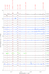 |
Fig. 1 Normalized barycentric-corrected spectra for F2, ordered by phase (shown on right), and with a constant offset in the y-direction. Red dashedvertical lines indicate rest wavelengths of significant lines. Spectra from SINFONI reduced by the same method are shown in black; those from KMOS are in blue and the spectrum from NIRSPEC is in green. |
3 Results
Amongst the 34 bright sources in our survey for which RVs could be measured, F2 stood out clearly. Figure 1 shows the spectra ordered by phase; the motion of the emission lines is readily apparent, especially near quadrature. The main emission lines are Brγ, He I 2.058 μm (strong P Cygni profile), He II 2.037, 2.189, 2.346 μm (weaker P Cygni profiles), C IV 2.079 μm, N III 2.247, 2.251 μm, Si IV 2.428 μm and the blended He I, N III, C III, O III complex at 2.112–2.115 μm. On the basisof these, Martins et al. (2008) classified F2 as WN8–9h. We should also note that, as discussed in Paper I, an N IV line contributes to the feature at 2.428 μm.
There is no clear evidence for line splitting, only for shifting of lines attributable to the assumed primary Wolf–Rayet component (with one exception). There are, however, some changes in the profiles of certain lines at different phases; for instance, Brγ (Fig. 2) shows the strongest and narrowest peak near eclipse of the secondary component, but is slightly weakened and broadened near quadratures, perhaps indicating a secondary emission component in this line. The N III 2.247, 2.251 μm pair of lines, not expected to be present in an OI star, do not show obvious profile changes with phase; they are perhaps the purest representative of the motion of the WNL component (Fig. 3).
Radial velocities were measured for the assumed primary WNL component from these two diagnostic features (Brγ and the N III pair), since they are strong, clearly visible in all spectra, in a wavelength region uncontaminated by strong residual telluric features, and expected to be relatively unaffected by a less massive companion. The final combined spectrum of F1 (see Paper I) was used as a template, since it is also a WNL star with a very similar spectral appearance to F2, and was not found to exhibit significant RV variability. Figure 4 shows the results; a full amplitude of variability around 350 km s−1 is clearly apparent from both features, far exceeding the uncertainties on the measurements. The NIRSPEC and KMOS spectra fit the trend of the SINFONI data quite well, despite having rather larger uncertainties. The curve from the N III lines is arguably of slightly greater amplitude than that from Brγ, but is also somewhat more scattered, owing to its lower S/N. Therefore, we used the average of the RVs measured from the two features for further analysis, and took the two original velocities as the uncertainty bounds for each new value (see Fig. 5 and Table 2). We note here a surprisingly large systemic velocity offset between F2 and F1 (about 60 km s−1); a preliminary determination of systemic velocities for all bright cluster members, to be finalized in Paper III, suggests that F2 is the outlier.
We argue that the spectra show clear evidence of secondary motion. The most promising feature is the C IV line at 2.079 μm, which appears weakly in emission in most spectra, and seems to vary in anti-phase with the other emission lines where present (Fig. 6). This is expected to be one of the strongest emission lines of an O supergiant (see Paper I), though it is also a weak emission feature in some of the Arches WNL spectra, including that of F1. An attempt was therefore made to measure the radial velocities of this line by cross-correlation, again using the combined spectrum of F1 as a template, and the results are shown in Table 2 and Fig. 7.
Anti-phase motion with amplitude greater than the primary is clearest from around phase 0.0 to 0.4, that is, when the primary is partially eclipsed by the secondary and shortly afterwards. One KMOS point at phase 0.160 deviates from the general trend; however, this data point and the one at phase 0.324 (corresponding to the weaker peak deblended from a double-peaked cross-correlation function) both match the expected velocities of the primary WNL star at these phases (Fig. 5), and so may be assumed to result from that component. This correspondence of primary RVs measured near quadrature from the Brγ, N III, and C IV lines supports our adoption of the same systemic velocity for the secondary RV curve, as shown in Fig. 7.
Around phases 0.5–0.6, the velocities are again close to those expected for the primary, which is unsurprising given that the secondary ispartially eclipsed here. Between phases 0.6 and 0.0 the velocities are more scattered, with those at phases 0.771 and 0.963 being close to the expected values for the primary, and other data points exhibiting a partial blueshift, though with amplitude smaller than that of the primary. It seems implausible that these points reflect the true motion of the secondary; they may instead correspond to an average of the primary and secondary velocities in a wind-collision region of the binary. By contrast, the data points from phases 0.0 to 0.4 can at worst only be underestimates of the true secondary velocities; it is hard to see a mechanism whereby they could systematically overestimate the amplitude of the secondary’s RV curve. The asymmetry of the velocities at the two quadratures may be caused by the primary wind wrapping round the secondary star; additional complications in measuring the blueshifted components of the C IV line at 2.079 μm are the red wing of the He I 2.058 μm line’s broadP Cygni profile, a possible contribution from a faint C IV line at 2.070 μm (clearly visible in WNL stars F6, F9, F14, and F16, and in O supergiants: see Paper I), and imperfectly-corrected telluric features (a deep telluric absorption band extends from around 2.04 to 2.08 μm).
Therefore, we tentatively identify a subset of the RVs measured from the C IV line at 2.079 μm as corresponding to the secondary component (Table 2), while acknowledging that these are likely torepresent minimum values. These data points suggest a full amplitude of variability around 500 km s−1. Given the scatter in primary velocities measured from two strong lines, the true uncertainties in our secondary velocities may be expected to be greater than those found through cross-correlation using a single weak line; we therefore doubled the size of these uncertainties for the remainder of the analysis, to make them comparable to the primary velocities.
The light curve of F2 (Fig. 8) also shows substantial variability, approaching 0.3 magnitudes (Table 3), where the typical scatter of the stars contributing to our composite reference star was just 0.015 magnitudes. One obviously deviant point in the light curve was excluded from further analysis; the error bars on other data points are probably too small, and the scatter of points about the average trend would give a more realistic estimate of the true uncertainties. We therefore multiplied all uncertainties by four for further analysis. It is nonetheless clear that the light curve has the appearance of a contact or near-contact binary, with narrow minima and continuous out-of-eclipse variability (see e.g. Lucy 1968). Despite this, the two minima are not separated by exactly half a cycle, suggesting a small eccentricity in the orbit, surprising in a contact system; this may be further supported by different heights of the two maxima, though the limited coverage of the second maximum makes this uncertain. The (small) apparent difference in depths of the two minima is probably not significant but a result of the partial coverage of these brief regions of the orbital cycle.
Period searches for the light curve by string length minimization indicate a minimum around 10.49 d (as found by Markakis et al. 2011), but with very similar values of the minimization statistic between 10.474 and 10.493 d, giving a mid-point of 10.483 ± 0.009 d. Using the primary RV curve alone, a much better-constrained minimum is found within the same range, between 10.481 and 10.485 d. A joint determination of the best period for both light and RV curves using string length minimization (after normalizing each curve by its amplitude) gives the same narrow minimum of 10.483 ± 0.002 d. This is because the RVs, though less numerous than the photometric data points, cover a far longer time base, and so provide a stronger constraint on the period (Fig. 9).
To check, we constructed a Lomb–Scargle periodogram of the primary RV data, searching for periods within a much wider range (0.5–100 d), which also finds a maximum peak at 10.483 d. The same search for the light curve data finds the strongest peak at around 5.25 d, that is, approximately half the period (Fig. 10). This is to be expected for eclipsing binary light curves with eclipses of similar depth, since the Lomb–Scargle method is equivalent to fitting sinusoidal functions to the time series, and binary curves are far more sinusoidal in shape when both eclipses are stacked on top of each other. We therefore took 10.483 ± 0.002 d as the period for the rest of the analysis.
We used the primary RV curve to determine which of the light curve minima to take as phase zero, and take BJD 2454679.553 as our reference zero point. All phases given in Tables 2 and 3 are assigned on the basis of this BJD0 and the period found as described above.
 |
Fig. 2 Brγ line at three phases, from SINFONI spectra: in black, near secondary eclipse (phase 0.550); in blue and red, near quadratures (phases 0.324 and 0.760). |
 |
Fig. 3 N III 2.247, 2.251 μm lines at three phases: in black, near secondary eclipse (phase 0.550); in blue and red, near quadratures (phases 0.324 and 0.760). |
 |
Fig. 4 RV curve for assumed WNL primary of F2, measured from Brγ (black) and N III 2.247, 2.251 μm (red) lines with F1 spectrum. SINFONI data are plotted as diamonds; KMOS and NIRSPEC as squares. |
 |
Fig. 5 Combined RV curve for the assumed WNL primary of F2. SINFONI data are plotted as diamonds; KMOS and NIRSPEC as squares. The solid blue horizontal line indicates the approximate systemic velocity (relative to F1); the dashed blue lines indicate the systemic velocities associated with the curves derived from the Brγ and N III lines separately, and may be taken as the uncertainty on the systemic velocity for the combined RV curve. |
 |
Fig. 6 C IV 2.079 μm line at threephases: in black, near secondary eclipse (phase 0.550); in blue and red, near quadratures (phases 0.324 and 0.760). Although the line is faint and noisy, we may observe that the main peak moves in anti-phase with the other lines (e.g. Figs. 2 and 3). |
RVs for F2 relative to F1.
 |
Fig. 7 RV curve measured from C IV 2.079 μm line. SINFONI data are plotted as diamonds and KMOS as squares. The horizontal line indicates the approximate systemic velocity (relative to F1) found from the primary curve (Fig. 5). Most of the data points indicate thevelocity corresponding to a single-peaked cross-correlation function, or the stronger peak of a deblended double-peaked function. However, the two red data points indicate a weaker but still significant peak in a deblended double-peaked function. The velocities taken as indicative of the behaviour of the secondary component are surrounded by the red dashed line, and are included in Table 2. |
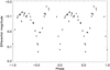 |
Fig. 8 Light curve for F2. The outlying point with larger uncertainty at phase 0.187 was associated with an incomplete observing run and has been excluded from further analysis. |
Differential photometry and phases for F2.
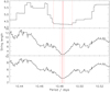 |
Fig. 9 String length values for candidate F2 periods near expected period: for the light curve data (upper panel), WNL radial velocities (middle panel) and combined light curve and radial velocities (lower panel). Dotted red vertical lines indicate the bounds of the region in each panel where the string length statistic is relatively constant and near its minimum value. Solid red vertical lines indicate the mid-point of these ranges. |
 |
Fig. 10 Lomb–Scargle periodograms for F2 WNL RV curve (upper panel) and light curve (lower panel), in range 0.5–100 d. The red horizontal lines indicate thresholds for false alarm probabilities of 0.10, 0.05, and 0.01, from bottom to top, in each panel. |
 |
Fig. 11 RV curves for F2 (primary in red, secondary in blue), with best-fit (unconstrained) PHOEBE models for both components overplotted. |
4 Modelling
We developed a binary model using the PHOEBE interface (Prša & Zwitter 2005) to the Wilson and Devinney eclipsing binary modelling code (Wilson & Devinney 1971). Two approaches were trialled: an unconstrained binary model, and one using constraints for a W UMa-type contact binary (i.e. both components share an effective temperature Teff and Kopal potential Ω) as the best available approximations to an assumed close, colliding-wind binary. Of course, it may be that the extended, semi-transparent atmosphere of the Wolf–Rayet component is what is actually in contact with the secondary, rather than its opaque core, and a more specialized approach would be required for optimal modelling (as in e.g. Perrier et al. 2009). However, here, given our rather limited data, we attempted merely to characterize the system in fairly broad terms.
The effective temperature for the two components (τ = 2/3) was taken as 34 000 K following spectral modelling (described below), or as Teff,1 = 34 100 K and Teff,2 = 33 800 K for the unconstrained model. Other starting assumptions were: bolometric albedo α = 0.5 and gravity darkening exponent β = 1.0 for radiative atmospheres (Hilditch 2001); a logarithmic limb darkening law; and orbital period and zero phase as given above. We first determined the eccentricity and argument of periastron by matching the synthetic curves to the well-defined observed light curve eclipse phases and the slight asymmetry of the observed primary RV curve; then the RV curves were used to estimate systemic velocity γ0, orbital separation a sin i (with orbital inclination i initially set to 90°) and mass ratio q ( , where M1 is the assumed WNL primary). Finally, the light curve shape was used to refine the orbital inclination i and Kopal potentials Ω1,2, with a being simultaneously adjusted to keep a sin i constant.
Owing to the relatively small number of data points of different origins and quality, and the differing usefulness of points at different phases in constraining the fits (e.g. during eclipse for the light curve, or at quadrature for the RV curves), manual adjustment was found to give a more convincing result than automated convergence of parameters (Figs. 11 and 12). Uncertainties in input and output parameters were estimated by varying input parameters from the best fit while maintaining a plausible match of the synthetic curves to the observed light and RV curves. The resulting best-fit parameters from the unconstrained binary model are given in Table 4.
An almost identical solution is obtained using the constraints for a contact binary, differing in a few details ultimately because of the shared temperature assumption. Crucially, we note that under both approaches the best fit requires approximately equal values of Ω1,2, just outside the Roche limit at the inner Lagrangian point (Ω(L1)) meaning that the components of F2 are almost in contact. No difference in the final component masses was produced by the two modelling approaches; the radii and hence luminosities of the components are very slightly smaller under the unconstrained model.
We were then able to disentangle the two components using KOREL (Hadrava 2012), implemented on the Virtual Observatory7. We used our derived period and epoch of periastron, together with our modelled mass ratio, semi-amplitude of the primary RV curve, and eccentricity as fixed constraints on the disentangling of the SINFONI spectra, since allowing these parameters to vary did not result in a convergent solution. We excluded the lower S/N spectrum at phase 0.034, and divided the other spectra into six wavelength sections to prevent undulation of the continuum.
The resulting spectra (rescaled using our preferred derived flux ratio between components, obtained as described below) are shown in Fig. 13. The primary component appears – as expected – to be a WNL star (Paper I classified it as WN8–9h). The secondary component shows features of an O hypergiant, for example, Br γ emission; HeI and He II absorption. Paper I placed the secondary in the context of seven other extreme O super- or hypergiants in the Arches, and gave it a provisional classification as O5–6 Ia+; F17 appearsto provide the closest spectral match. This successful disentangling, producing a pair of spectra closely resembling other massive cluster members, gives support to the validity of our binary modelling and the pair of RV curves on which the model depends.
Further confirmation was sought through a series of spectral fitting tests, using high S/N SINFONI spectra at four phases: near the two eclipses and near the two quadratures. Levenberg–Marquardt fits were carried out for more than 400 000 combinations of possible primary and secondary spectra, drawn from two grids of CMFGEN models (Hillier & Miller 1998, 1999), self-computed to encompass the parameter domains of interest. A WNL grid for the primary covered Teff from 30 000 to 39 000 K, log g from 3.2 to 3.7, wind density parameter log Q from −11.8 to −10.5, He/H from 0.2 to 1.0 (number), and the clumping factor fcl from 1 to 0.03. The secondary grid consisted of the primary grid (to investigate the possibility of two WNLs) combined with an O star grid covering dwarf, giant and supergiant domains; this led to a range in log g from 3.1 to 4.2 and in log Q from −12.3 to −10.5. Largely complete model atoms for C, N, O, Si, and S were assumed, to account for the infrared transitions among high-lying levels present in the K band. In the fitting tests, the flux ratio between the two components (F12) and their RVs could also be estimated, and specific lines could be given more weight in the fitting (e.g. the CIV line at 2.079 μm, of particular relevance for the secondary component).
By fitting all four phases simultaneously, and leaving F12 and the RVs as free parameters, good matches were achieved to all four observed spectra, using a flux ratio of 1.60, Teff~34 000 K and log g ~ 3.3 for both components (Fig. 14). (The blend of N IV with Si IV at 2.428 μm limits the sensitivity of this otherwise useful line to log g for the primary; He II lines in the secondary are consistent with log g between ~3.1 and 3.3 however.) We should note that the relative velocity of the two components is ill-constrained near secondary eclipse where the secondary’s weaker features are largely obscured. An alternative approach was to fix the relative velocities of the two components (using the observed radial velocities and their best-fit modelled curves in Fig. 11) and leave the flux ratio free. This approach yielded nearly identical spectral models to the first method (though with slightly poorer fits to the combined spectra), and a rather higher F12 of 1.88 (Fig. 15).
Having obtained best-fit model spectra very similar to the disentangled spectra, a final fit was carried out to each disentangled component separately, assuming a flux ratio of 1.60. The resulting fits are shown in Fig. 13 and provide good matches almost everywhere except around the He I 2.058 μm line, where strong and variable telluric absorption is almost impossible to remove cleanly. The final parameters of the component models are given in Table 5.
To provide an independent estimate of the luminosities of the components of F2, SED modelling of the system during secondary eclipse was carried out by combining the primary and secondary best-fit models, assuming a particular K-band flux ratio between the components, and using the difference in system magnitude relative to the out-of-eclipse magnitude of 0.264 (obtained from the fitted light curve). The observed magnitudes we used, adjusted for phase, are given in Table 6. Given the uncertainty over the appropriate extinction prescription to use, a variety of extinction laws were explored, as described for the wider cluster in Paper I. The two main types were α-laws (i.e. Aλ =  , where Ak0 is the monochromatic value at 2.159 μm = λ0 in 2MASS Ks), and Moneti’s law, where RV is assumed to be 3.1, and Ak0 is derived. Further tests were performed assuming fixed α values from literature or by using a two-α approach.
Figure 16 and Table 5 show the best-fit results for the two main extinction approaches, assuming F12 = 1.60. It is apparent that both extinction prescriptions are capable of fitting the observed magnitudes well, but they lead to differences in Ak0 of almost two magnitudes for such a heavily-reddened object as F2, which translates into 0.8 dex in log L. The plot also shows the degeneracy in the extinction in the 4.1–4.4 log λ region, which would require medium-width filters at 1.0 and 1.1 μm to break. However, only the Moneti approach yields luminosities roughly compatible with our binary modelling results (Table 4), even allowing for uncertainties in the SED-modelled log  of around +0.08, −0.04 dex. Stellar radii below 20 R⊙ would also imply implausibly low masses in the context of the Wolf–Rayet members of the Arches.
Given the substantial mass-loss expected for a Wolf–Rayet star through stellar wind (directly supported in the case of F2 by the P Cygni profiles of some lines, and by model atmosphere analysis), it is useful to compare our model results with the expected mass evolution of such a star. Figure 17 shows Geneva evolutionary tracks (Ekström et al. 2012) for stars with initial masses 60–300 M⊙, including rotating models where available. Although these models do not include binary interactions, they should give some indication of the maximum mass loss expected for the primary, and thus its minimum plausible current mass. Using an age for the Arches of 2.5 ± 0.5 Myr (Figer et al. 2002; Martins et al. 2008), we can see that the most massive stars would already have completed their WNL stage, while the least massive would not yet have reached it8. With the age of 3.5 ± 0.7 Myr proposed by Schneider et al. (2014), the only plausible candidates would be the rotating 60, 85, and 120 M⊙,init tracks, or (very briefly) the non-rotating 60 and 85 M⊙,init tracks. Combining these age constraints would allow a current mass between ~150 and ~25 M⊙; if we prefer rotating models for a binary configuration, the lowest possible current mass for the primary would be ~40 M⊙.
We may also investigate the temperature and luminosity of F2’s primary according to the model. Figure 18 shows an HR diagram for the WNL phases of the same evolutionary tracks, where these overlap with the expected age range for the Arches (2.0–4.2 Myr). Also shown here is the location of the modelled F2 primary, using the luminosity found from binary modelling. We observe that it lies close to the start of the rotating 120 M⊙,init track (in cyan). Referring back again to Fig. 17, and matching its modelled mass of 82 ± 12 M⊙ with this evolutionary track, an age of 2.6 Myr is supported. If the slightly higher luminosity found from SED fitting, using the Moneti law, is preferred, the 150 M⊙,init track would be supported instead, suggesting an age closer to 2.5 Myr.
At this age, the secondary’s modelled current mass of 60 ± 8 M⊙ would place it in the region of the 60 and 85 M⊙,init tracks, prior to the WNL stage or possibly just at the start of it (using the rotating 85 M⊙,init track). However, it should be noted that simulations in Groh et al. (2014) were unable to generate an O hypergiant phase from a 60 M⊙,init star; this may indicate that F2’s secondary was originally more massive. R2 is perhaps rather large and hence log  is rather high for an O hypergiant secondary: comparable single stars studied in Martins et al. (2008) (F10 and F15) are modelled as having radii ~30 R⊙. However, aninflated secondary radius is expected in lower-mass contact binaries due to the shared envelope (Lohr et al. 2015), and a comparable mechanism may be in operation here.
 |
Fig. 12 Light curve for F2 with best-fit (unconstrained) PHOEBE model overplotted in red. |
Best-fit system and stellar component parameters for F2 from (unconstrained) binary modelling.
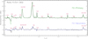 |
Fig. 13 Disentangled spectra for F2 primary and secondary components (black lines) with best-fit model spectra overplotted (green and blue dashed lines). |
 |
Fig. 14 Best-fit model spectra for primary (pink), secondary (blue), and combined (yellow) components of F2, matched to observed spectra (black) at four phases. Relative velocities of the primary and secondary were a free parameter under this modelling approach. |
 |
Fig. 15 Best-fit model spectra for F2, as in Fig. 14, but with relative velocities of the primary and secondary fixed to values found from binary modelling. |
Best-fit stellar component parameters for F2 from CMFGEN model fitting to disentangled spectra and from SED fitting.
Phase-corrected magnitudes used for SED fitting.
5 Discussion
The most plausible model for F2, based on available data, appears to be a near-contact eclipsing SB2 binary containing a ~80 M⊙ WN8–9h component with a strong stellar wind, and a luminous ~60 M⊙ O-type secondary. The orbit seems to be not yet quite circularized, but some interaction is probable in the form of colliding winds, which may explain the behaviour of the C IV line at 2.079 μm around and after the secondary eclipse. Such colliding winds are supported by detections near the location of F2 of X-ray source A6 (Wang et al. 2006), and radio source AR10 (Lang et al. 2005) with log Ṁ of −4.72 M⊙ yr−1 (where we found log Ṁ of −4.29 M⊙ yr−1); non-detection of AR10 in Lang et al. (2001) may also indicate radio variability.
F2 thus seems comparable with a handful of very massive binaries containing WNL stars as primaries. WR21a (Benaglia et al. 2005; Niemela et al. 2008; Tramper et al. 2016) is particularly similar: an X-ray bright, colliding-wind, eccentric spectroscopic O3/WN5ha+O3 binary with P = 31.7 d, and with absolute masses for its components of ~104 and 58 M⊙. Moreover, the secondary’s lines were only detected from disentangled high-resolution spectra. WR22 (Rauw et al. 1996; Schweickhardt et al. 1999; Gräfener & Hamann 2008) is a much longer-period binary containing rather less massive WN7+abs and O9 components, of which Schweickhardt et al. (1999) noted “the absorptions from the companion are extremely weak and they can only be detected in spectra with a very high signal to noise ratio”. An even longer period and highly eccentric binary, R145 (Schnurr et al. 2009; Shenar et al. 2017), has recently been disentangled to reveal WN6h and O3.5If*/WN7 components, with primary and secondary masses ~55 M⊙ (from orbital and polarimetric analysis), or nearer ~80 M⊙ (using quasi-homogeneous evolution tracks). WR20a, (Rauw et al. 2004; Bonanos et al. 2004; Nazé et al. 2008), also a colliding-wind binary, has nearly equal-mass WN6ha components (82 and 83 M⊙) and is a clear SB2 with a much shorter period than F2 (3.7 d), but its deeply-eclipsing light curve shows a strong resemblance to F2, and was also modelled as a contact or near-contact system. Possibly more massive than F2 is the P = 3.8 d system NGC 3603-A1 (Moffat et al. 2004; Schnurr et al. 2008) containing a WN6ha and a secondary of similar spectral type, although the RVs for its secondary were difficult to determine due to colliding-wind features and blending of the extremely broad lines used, resulting in 20–30% uncertainties on masses. Even more challenging is R144 (Sana et al. 2013), which appears to be an SB2 with very high luminosity (log  ), but for which no clear period has yet been determined.
In contrast, WR29 (Niemela & Gamen 2000; Gamen et al. 2009) is a WN7h+O eclipsing binary in which the O star is found to be more massive than the Wolf–Rayet (53 and 42 M⊙). Its light curve appears very different from that of F2, with primary and secondary eclipses and maxima of different depths and heights. Furthermore, a number of absorption lines from the O star were readily observed in its spectra, superimposed on the Wolf–Rayet’s emission lines. A less massive system of this type appears to be WR77o (Negueruela & Clark 2005; Crowther et al. 2006; Koumpia & Bonanos 2012), with a ~43 M⊙ O-type primary and a ~16 M⊙ WN7o (hydrogen-depleted) secondary; the O star’s absorption lines were not detected there in spite of its greater temperature and radius, but the system is still not a good comparator for the highly luminous and hydrogen-rich F2. Details for these and other WNL binary members are given in Table 7.
It is noteworthy that the only Galactic binaries on that list which are currently more massive than F2 (WR21a, WR20a, and NGC 3603-A1) are considerably younger (1–2 Myr), and so may be expected to be closer to their initial masses. F2, with an age around 2.6 Myr, and likely initial primary mass between 120 and 150 M⊙, may have been the most massive binary in the Galaxy at its formation.
In any case, the binarity of F2 is indisputable given its photometric and spectroscopic variability with a common period. Might there be other binaries in the Arches? Significant photometric variability was not observed in any bright Arches targets besides F2. However, Wang et al. (2006) identified three other bright X-ray sources in the cluster: F6, F7, and F9, and suggested these were produced by “colliding stellar winds in massive star close binaries”; of these, F6 and F7 were also detected as bright radio-variable sources in Lang et al. (2001, 2005) (F9 was not included in their survey). Our preliminary spectroscopic results for these three objects (see Paper III) do provide some support for significant RV variations, though with far lower amplitudes of variability than F2. More convincingly, the OIf+ hypergiant F15 and the O supergiant F35 exhibit highly significant variability with Δ RV around 75 and 220 km s−1 respectively. Forthcoming scheduled observations of these and other Arches targets should allow us to confirm their spectroscopic variability status, and establish whether any variability is periodic and plausibly associated with binarity.
The demonstrable binarity of at least one very massive member of the Arches may present a challenge to Schneider et al. (2014), who argue that the most massive 9 ± 3 stars in this cluster are expected to be rejuvenated products of binary mass transfer and merger. Such rejuvenation is proposed as an explanation for the finding of Martins et al. (2008) that “the most massive stars are slightly younger than the less massive stars”, which could otherwise be understood as being caused by an extended star formation period. Schneider et al. determine a cluster age of 3.5 ± 0.7 Myr on this basis, which barely overlaps with our estimated age for F2 of 2.6 Myr, at least using evolutionary models for single stars. Such models may not be fully appropriate for a near-contact system, in which some interaction is very likely to have occurred already, at least between the component winds; however, in the current absence of suitable evolutionary models for such massive binary components, and given that interaction has apparently not yet been sufficient to circularise the binary orbit, we regard them as providing a usable approximation.
It is of course possible that F2 formed more recently than the rest of the cluster, though this explanation would be less tenable if other spectroscopically-variable Arches members prove to be binaries as well. We may also note that the spectrum of F2’s primary is very similar to those of the other highly luminous WNL members of the cluster (Paper I); if the others had been “rejuvenated” while this one had not, we might expect a greater difference. In Paper I, we found a smooth progression in spectral morphology from WNLh stars through OIf+ hypergiants to O supergiants, giants and arguably dwarfs, supporting coevality. Despite our survey reaching a magnitude at which they should have been detectable, no more evolved objects such as hydrogen-depleted WNE or WC stars were observed, nor transitional objects such as luminous blue variables, as are seen in the slightly older Quintuplet cluster (Geballe et al. 2000).
 |
Fig. 16 Best-fit SEDs for F2 using different extinction prescriptions. In black, the preferred primary and secondary models are combined, with final luminosities of log |


 |
Fig. 17 Mass over time for candidate primary component of F2, from latest Geneva evolutionary models with Z = 0.014. Initial masses are shown (in solar masses) next to each track on the left; for the 60, 85, and 120 M⊙ tracks, bothrotating and non-rotating models are shown (the rotating models are in red, yellow, and cyan respectively, and have greater duration than the corresponding non-rotating versions in black, orange and green); for higher initial masses, only non-rotating models are available. Each track follows the life of a star to the end of the C burning stage (dotted lines); WNL phases, as defined in Georgy et al. (2012), are shown in thicker solid lines. |
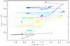 |
Fig. 18 HR diagram of candidate Geneva models for F2 primary star. Partial evolutionary tracks are shown, for the WNL stage at ages 2–4.2 Myr. Each track has the same colour as in Fig. 17. The cross indicates the luminosity and temperature(with uncertainties) of the primary of F2 from our binary and spectral models respectively. |
Published parameters for comparable binaries with dynamical mass estimates, containing WNL components.
6 Conclusions
Our spectroscopic survey of the most massive and luminous members of the Arches cluster revealed one source which exhibits significant and substantial RV variability: F2, classified as WN8–9h by Martins et al. (2008). Further archival spectra indicated that the velocities vary sinusoidally, with a period of 10.483 d, matching the light curve period found by Markakis et al. (2011) for the same source in a photometric survey. Re-reducing the photometry yielded a light curve typical of a contact or near-contact eclipsing binary, with a small eccentricity. Radio and X-ray observations also suggested that F2 could be a colliding-wind massive binary.
We have presented preliminary models for this system as an SB2 near-contact eclipsing binary. The secondary RV curve is only partially determined by a single faint line moving in anti-phase with the WNL primary. Combining the RV and light curves, and using an effective temperature obtained from spectral fitting, we modelled the system as having M1 = 82 ± 12 M⊙, M2 = 60 ± 8 M⊙. The primary’s modelled properties are consistent with a rotating 120 M⊙,init evolutionary track and an age of 2.6 Myr, though an initial mass as high as 150 M⊙ and age nearer 2.5 Myr is also consistent with our SED-modelled luminosities. From spectral disentangling and independent searches for best-fitting template spectra from a large grid of CMFGEN models, the secondary is most likely an O hypergiant similar to others in the Arches (O5–6 Ia+).
F2 therefore appears to be one of a small set of very massive binaries containing Wolf–Rayet primaries, and is perhaps the most massive binary in the Galaxy in terms of initial mass, since other systems with higher dynamical mass estimates are in much younger clusters and so will have lost less mass. It is also the first confirmed binary in the Arches cluster, potentially conflicting with an argument of Schneider et al. (2014) that the most massive members of the Arches are expected to be the products of binary interaction and merger, and that the cluster itself is around 3.5 Myr old. F2 is one of four hard, bright X-ray sources within the Arches that have been interpreted as colliding-wind binaries; the confirmation of its binary nature strongly implies that the other three sources are similar systems. Moreover, our spectroscopic survey has revealed a number of additional RV variables, although further observations will be required to characterize these fully (Paper III). A synthesis of these findings hints at a rich binary population within the Arches.
The confirmation of the binary nature of F2 alone has important implications for the global properties of the Arches, potentially allowing us to calibrate the mass–luminosity relationship and consequently determine the cluster’s (initial) mass function and integrated mass. In turn, these parameters will enable us to place constraints on the upper mass limit of stars; the apparently pre-interaction configuration of F2 also has important implications for the formation of very massive stars, suggesting that they do not all form via binary mass transfer and/or merger. Finally, determination of the frequency of occurrence of such very massive binaries will provide critical observational constraints for population synthesis modelling of the progenitors of massive, coalescing, relativistic binaries, and gravitational wave sources.
Acknowledgements
Based on observations collected at the European Organisation for Astronomical Research in the Southern Hemisphere under ESO programmes 075.D-0736, 081.D-0480, 087.D-0317, 087.D-0342, 091.D-0187, and 093.D-0306, and based on data obtained from the ESO Science Archive Facility under request numbers 155505, 155514, 189886, 190865, 283402, 283411, 283415, 283417, and 283512. This research was supported by the Science and Technology Facilities Council. FN acknowledges financial support through Spanish grants ESP2015-65597-C4-1-R and ESP2017-86582-C4-1-R (MINECO/FEDER). We are grateful to Dong Hui for assistance with the reduction of archival photometric data for our spectral energy distribution modelling, and to Fabrice Martins for the kind provision of his SINFONI reduced data cubes from 2005, as well as his design of the original SINFONI observing strategy used for the Arches.
References
- Abbott, B. P., The LIGO Scientific Collaboration, & the Virgo Collaboration 2016, Phys. Rev. Lett., 116, 061102 [Google Scholar]
- Benaglia, P., Romero, G. E., Koribalski, B., & Pollock, A. M. T. 2005, A&A, 440, 743 [NASA ADS] [CrossRef] [EDP Sciences] [Google Scholar]
- Blum, R. D., Schaerer, D., Pasquali, A., et al. 2001, AJ, 122, 1875 [NASA ADS] [CrossRef] [Google Scholar]
- Bonanos, A. Z., Stanek, K. Z., Udalski, A., et al. 2004, ApJ, 611, L33 [NASA ADS] [CrossRef] [Google Scholar]
- Bonnet, H., Abuter, R., Baker, A., et al. 2004, The Messenger, 117, 17 [NASA ADS] [Google Scholar]
- Clark, J. S., Ritchie, B. W., Negueruela, I., et al. 2011, A&A, 531, A28 [NASA ADS] [CrossRef] [EDP Sciences] [Google Scholar]
- Clark, J. S., Lohr, M. E., Najarro, F., Dong, H., & Martins, F. 2018, A&A, 617, A65 (Paper I) [Google Scholar]
- Cotera, A. S., Erickson, E. F., Colgan, S. W. J., et al. 1996, ApJ, 461, 750 [NASA ADS] [CrossRef] [Google Scholar]
- Crowther, P. A., Hadfield, L. J., Clark, J. S., Negueruela, I., & Vacca, W. D. 2006, MNRAS, 372, 1407 [NASA ADS] [CrossRef] [Google Scholar]
- Davies, R. I., Agudo Berbel, A., Wiezorrek, E., et al. 2013, A&A, 558, A56 [NASA ADS] [CrossRef] [EDP Sciences] [Google Scholar]
- Dong, H., Wang, Q. D., Cotera, A., et al. 2011, MNRAS, 417, 114 [NASA ADS] [CrossRef] [Google Scholar]
- Dong, H., Schödel, R., Williams, B. F., et al. 2018, ApJ, submitted [Google Scholar]
- Dworetsky, M. M. 1983, MNRAS, 203, 917 [NASA ADS] [Google Scholar]
- Eastman, J., Siverd, R., & Gaudi, B. S. 2010, PASP, 122, 935 [NASA ADS] [CrossRef] [Google Scholar]
- Eisenhauer, F., Abuter, R., Bickert, K., et al. 2003, SPIE Conf. Ser., 4841, 1548 [Google Scholar]
- Ekström, S., Georgy, C., Eggenberger, P., et al. 2012, A&A, 537, A146 [NASA ADS] [CrossRef] [EDP Sciences] [Google Scholar]
- Figer, D. F. 2005, Nature, 434, 192 [NASA ADS] [CrossRef] [PubMed] [Google Scholar]
- Figer, D. F., Najarro, F., Gilmore, D., et al. 2002, ApJ, 581, 258 [NASA ADS] [CrossRef] [Google Scholar]
- Gamen, R., Gosset, E., Morrell, N. I., et al. 2008, Rev. Mex. Astron. Astrofis, 33, 91 [Google Scholar]
- Gamen, R. C., Fernández-Lajús, E., Niemela, V. S., & Barbá, R. H. 2009, A&A, 506, 1269 [NASA ADS] [CrossRef] [EDP Sciences] [Google Scholar]
- Geballe, T. R., Najarro, F., & Figer, D. F. 2000, ApJ, 530, L97 [NASA ADS] [CrossRef] [PubMed] [Google Scholar]
- Georgy, C., Ekström, S., Meynet, G., et al. 2012, A&A, 542, A29 [NASA ADS] [CrossRef] [EDP Sciences] [Google Scholar]
- Gräfener, G.,& Hamann, W.-R. 2008, A&A, 482, 945 [NASA ADS] [CrossRef] [EDP Sciences] [Google Scholar]
- Groh, J. H., Meynet, G., Ekström, S., & Georgy, C. 2014, A&A, 564, A30 [NASA ADS] [CrossRef] [EDP Sciences] [Google Scholar]
- Hadrava, P. 2012, IAU Symp., 282, 351 [Google Scholar]
- Hilditch, R. W. 2001, An Introduction to Close Binary Stars (Cambridge: Cambridge University Press) [CrossRef] [Google Scholar]
- Hillier, D. J., & Miller, D. L. 1998, ApJ, 496, 407 [NASA ADS] [CrossRef] [Google Scholar]
- Hillier, D. J., & Miller, D. L. 1999, ApJ, 519, 354 [NASA ADS] [CrossRef] [Google Scholar]
- Horne, J. H., & Baliunas, S. L. 1986, ApJ, 302, 757 [NASA ADS] [CrossRef] [Google Scholar]
- Hur, H., Sung,H., & Bessell, M. S. 2012, AJ, 143, 41 [NASA ADS] [CrossRef] [Google Scholar]
- Koumpia, E., & Bonanos, A. Z. 2012, A&A, 547, A30 [NASA ADS] [CrossRef] [EDP Sciences] [Google Scholar]
- Lang, C. C., Goss, W. M., & Rodríguez, L. F. 2001, ApJ, 551, L143 [NASA ADS] [CrossRef] [Google Scholar]
- Lang, C. C., Johnson, K. E., Goss, W. M., & Rodríguez, L. F. 2005, AJ, 130, 2185 [Google Scholar]
- Lenzen, R., Hartung, M., Brandner, W., et al. 2003, SPIE Conf. Ser., 4841, 944 [Google Scholar]
- Lohr, M. E., Norton, A. J., Gillen, E., et al. 2015, A&A, 578, A103 [NASA ADS] [CrossRef] [EDP Sciences] [Google Scholar]
- Lomb, N. R. 1976, Ap&SS, 39, 447 [NASA ADS] [CrossRef] [Google Scholar]
- Lucy, L. B. 1968, ApJ, 153, 877 [NASA ADS] [CrossRef] [Google Scholar]
- Markakis, K., Bonanos, A. Z., Pietrzynski, G., Macri, L., & Stanek, K. Z. 2011, IAU Symp., 272, 298 [NASA ADS] [Google Scholar]
- Markakis, K., Bonanos, A. Z., Pietrzynski, G., Macri, L., & Stanek, K. Z. 2012, IAU Symp., 282, 454 [NASA ADS] [Google Scholar]
- Martins, F., & Palacios, A. 2017, A&A, 598, A56 [NASA ADS] [CrossRef] [EDP Sciences] [Google Scholar]
- Martins, F., Hillier, D. J., Paumard, T., et al. 2008, A&A, 478, 219 [NASA ADS] [CrossRef] [EDP Sciences] [Google Scholar]
- Moffat, A. F. J., Poitras, V., Marchenko, S. V., et al. 2004, AJ, 128, 2854 [NASA ADS] [CrossRef] [Google Scholar]
- Nagata, T., Woodward, C. E., Shure, M., & Kobayashi, N. 1995, AJ, 109, 1676 [NASA ADS] [CrossRef] [Google Scholar]
- Najarro, F., Figer, D. F., Hillier, D. J., Geballe, T. R., & Kudritzki, R. P. 2009, ApJ, 691, 1816 [NASA ADS] [CrossRef] [Google Scholar]
- Nazé, Y., Rauw, G., & Manfroid, J. 2008, A&A, 483, 171 [NASA ADS] [CrossRef] [EDP Sciences] [Google Scholar]
- Negueruela, I., & Clark, J. S. 2005, A&A, 436, 541 [NASA ADS] [CrossRef] [EDP Sciences] [Google Scholar]
- Niemela, V. S., & Gamen, R. C. 2000, A&A, 362, 973 [NASA ADS] [Google Scholar]
- Niemela, V. S., Gamen, R. C., Barbá, R. H., et al. 2008, MNRAS, 389, 1447 [NASA ADS] [CrossRef] [Google Scholar]
- Patrick, L. R., Evans, C. J., Davies, B., et al. 2015, ApJ, 803, 14 [NASA ADS] [CrossRef] [Google Scholar]
- Perrier, C., Breysacher, J., & Rauw, G. 2009, A&A, 503, 963 [NASA ADS] [CrossRef] [EDP Sciences] [Google Scholar]
- Prša, A., & Zwitter, T. 2005, ApJ, 628, 426 [NASA ADS] [CrossRef] [Google Scholar]
- Rauw, G., Vreux, J.-M., Gosset, E., et al. 1996, A&A, 306, 771 [NASA ADS] [Google Scholar]
- Rauw, G., De Becker, M., Nazé, Y., et al. 2004, A&A, 420, L9 [NASA ADS] [CrossRef] [EDP Sciences] [Google Scholar]
- Ritchie, B. W., Clark, J. S., Negueruela, I., & Crowther, P. A. 2009, A&A, 507, 1585 [NASA ADS] [CrossRef] [EDP Sciences] [Google Scholar]
- Ritchie, B. W., Clark, J. S., Negueruela, I., & Langer, N. 2010, A&A, 520, A48 [NASA ADS] [CrossRef] [EDP Sciences] [Google Scholar]
- Rousset, G., Lacombe, F., Puget, P., et al. 2003, SPIE Conf. Ser., 4839, 140 [Google Scholar]
- Sana, H., van Boeckel, T., Tramper, F., et al. 2013, MNRAS, 432, 26 [Google Scholar]
- Scargle, J. D. 1982, ApJ, 263, 835 [NASA ADS] [CrossRef] [Google Scholar]
- Schneider, F. R. N., Izzard, R. G., de Mink, S. E., et al. 2014, ApJ, 780, 117 [NASA ADS] [CrossRef] [Google Scholar]
- Schnurr, O., Casoli, J., Chené, A.-N., Moffat, A. F. J., & St-Louis, N. 2008, MNRAS, 389, L38 [NASA ADS] [CrossRef] [Google Scholar]
- Schnurr, O., Moffat, A. F. J., Villar-Sbaffi, A., St-Louis, N., & Morrell, N. I. 2009, MNRAS, 395, 823 [NASA ADS] [CrossRef] [Google Scholar]
- Schweickhardt, J., Schmutz, W., Stahl, O., Szeifert, T., & Wolf, B. 1999, A&A, 347, 127 [NASA ADS] [Google Scholar]
- Sharples, R., Bender, R., Agudo Berbel, A., et al. 2013, The Messenger, 151, 21 [NASA ADS] [Google Scholar]
- Shenar, T., Richardson, N. D., Sablowski, D. P., et al. 2017, A&A, 598, A85 [NASA ADS] [CrossRef] [EDP Sciences] [Google Scholar]
- Stolte, A., Grebel, E. K., Brandner, W., & Figer, D. F. 2002, A&A, 394, 459 [NASA ADS] [CrossRef] [EDP Sciences] [Google Scholar]
- Tramper, F., Sana, H., Fitzsimons, N. E., et al. 2016, MNRAS, 455, 1275 [NASA ADS] [CrossRef] [Google Scholar]
- Wang, Q. D., Dong, H., & Lang, C. 2006, MNRAS, 371, 38 [NASA ADS] [CrossRef] [Google Scholar]
- Wilson, R. E., & Devinney, E. J. 1971, ApJ, 166, 605 [NASA ADS] [CrossRef] [Google Scholar]
ESO proposals 087.D-0317 and 091.D-0187, PI J. S. Clark.
ESO proposal 075.D-0736, PI T. Paumard.
ESO proposal 087.D-0342, PI G. Pietrzynski.
ESO proposal 093.D-0306, PI J. S. Clark.
ESO proposal 081.D-0480, PI G. Pietrzynski.
However, following Martins & Palacios (2017), caution is required in using the definition of a Wolf–Rayet/WNL phase in an evolutionary model, based on abundances, to evaluate a spectroscopically-defined WNL; the two will not necessarily be consistent.
All Tables
Best-fit system and stellar component parameters for F2 from (unconstrained) binary modelling.
Best-fit stellar component parameters for F2 from CMFGEN model fitting to disentangled spectra and from SED fitting.
Published parameters for comparable binaries with dynamical mass estimates, containing WNL components.
All Figures
|
Fig. 1 Normalized barycentric-corrected spectra for F2, ordered by phase (shown on right), and with a constant offset in the y-direction. Red dashedvertical lines indicate rest wavelengths of significant lines. Spectra from SINFONI reduced by the same method are shown in black; those from KMOS are in blue and the spectrum from NIRSPEC is in green. |
| In the text | |
|
Fig. 2 Brγ line at three phases, from SINFONI spectra: in black, near secondary eclipse (phase 0.550); in blue and red, near quadratures (phases 0.324 and 0.760). |
| In the text | |
|
Fig. 3 N III 2.247, 2.251 μm lines at three phases: in black, near secondary eclipse (phase 0.550); in blue and red, near quadratures (phases 0.324 and 0.760). |
| In the text | |
|
Fig. 4 RV curve for assumed WNL primary of F2, measured from Brγ (black) and N III 2.247, 2.251 μm (red) lines with F1 spectrum. SINFONI data are plotted as diamonds; KMOS and NIRSPEC as squares. |
| In the text | |
|
Fig. 5 Combined RV curve for the assumed WNL primary of F2. SINFONI data are plotted as diamonds; KMOS and NIRSPEC as squares. The solid blue horizontal line indicates the approximate systemic velocity (relative to F1); the dashed blue lines indicate the systemic velocities associated with the curves derived from the Brγ and N III lines separately, and may be taken as the uncertainty on the systemic velocity for the combined RV curve. |
| In the text | |
|
Fig. 6 C IV 2.079 μm line at threephases: in black, near secondary eclipse (phase 0.550); in blue and red, near quadratures (phases 0.324 and 0.760). Although the line is faint and noisy, we may observe that the main peak moves in anti-phase with the other lines (e.g. Figs. 2 and 3). |
| In the text | |
|
Fig. 7 RV curve measured from C IV 2.079 μm line. SINFONI data are plotted as diamonds and KMOS as squares. The horizontal line indicates the approximate systemic velocity (relative to F1) found from the primary curve (Fig. 5). Most of the data points indicate thevelocity corresponding to a single-peaked cross-correlation function, or the stronger peak of a deblended double-peaked function. However, the two red data points indicate a weaker but still significant peak in a deblended double-peaked function. The velocities taken as indicative of the behaviour of the secondary component are surrounded by the red dashed line, and are included in Table 2. |
| In the text | |
|
Fig. 8 Light curve for F2. The outlying point with larger uncertainty at phase 0.187 was associated with an incomplete observing run and has been excluded from further analysis. |
| In the text | |
|
Fig. 9 String length values for candidate F2 periods near expected period: for the light curve data (upper panel), WNL radial velocities (middle panel) and combined light curve and radial velocities (lower panel). Dotted red vertical lines indicate the bounds of the region in each panel where the string length statistic is relatively constant and near its minimum value. Solid red vertical lines indicate the mid-point of these ranges. |
| In the text | |
|
Fig. 10 Lomb–Scargle periodograms for F2 WNL RV curve (upper panel) and light curve (lower panel), in range 0.5–100 d. The red horizontal lines indicate thresholds for false alarm probabilities of 0.10, 0.05, and 0.01, from bottom to top, in each panel. |
| In the text | |
|
Fig. 11 RV curves for F2 (primary in red, secondary in blue), with best-fit (unconstrained) PHOEBE models for both components overplotted. |
| In the text | |
|
Fig. 12 Light curve for F2 with best-fit (unconstrained) PHOEBE model overplotted in red. |
| In the text | |
|
Fig. 13 Disentangled spectra for F2 primary and secondary components (black lines) with best-fit model spectra overplotted (green and blue dashed lines). |
| In the text | |
|
Fig. 14 Best-fit model spectra for primary (pink), secondary (blue), and combined (yellow) components of F2, matched to observed spectra (black) at four phases. Relative velocities of the primary and secondary were a free parameter under this modelling approach. |
| In the text | |
|
Fig. 15 Best-fit model spectra for F2, as in Fig. 14, but with relative velocities of the primary and secondary fixed to values found from binary modelling. |
| In the text | |
|
Fig. 16 Best-fit SEDs for F2 using different extinction prescriptions. In black, the preferred primary and secondary models are combined, with final luminosities of log |
| In the text | |
|
Fig. 17 Mass over time for candidate primary component of F2, from latest Geneva evolutionary models with Z = 0.014. Initial masses are shown (in solar masses) next to each track on the left; for the 60, 85, and 120 M⊙ tracks, bothrotating and non-rotating models are shown (the rotating models are in red, yellow, and cyan respectively, and have greater duration than the corresponding non-rotating versions in black, orange and green); for higher initial masses, only non-rotating models are available. Each track follows the life of a star to the end of the C burning stage (dotted lines); WNL phases, as defined in Georgy et al. (2012), are shown in thicker solid lines. |
| In the text | |
|
Fig. 18 HR diagram of candidate Geneva models for F2 primary star. Partial evolutionary tracks are shown, for the WNL stage at ages 2–4.2 Myr. Each track has the same colour as in Fig. 17. The cross indicates the luminosity and temperature(with uncertainties) of the primary of F2 from our binary and spectral models respectively. |
| In the text | |
Current usage metrics show cumulative count of Article Views (full-text article views including HTML views, PDF and ePub downloads, according to the available data) and Abstracts Views on Vision4Press platform.
Data correspond to usage on the plateform after 2015. The current usage metrics is available 48-96 hours after online publication and is updated daily on week days.
Initial download of the metrics may take a while.