| Issue |
A&A
Volume 617, September 2018
|
|
|---|---|---|
| Article Number | A77 | |
| Number of page(s) | 11 | |
| Section | Interstellar and circumstellar matter | |
| DOI | https://doi.org/10.1051/0004-6361/201731975 | |
| Published online | 18 September 2018 | |
High-J CO emission spatial distribution and excitation in the Orion Bar★,★★
1
I. Physikalisches Institut der Universität zu Köln,
Zülpicher Straße 77,
50937
Köln,
Germany
e-mail: This email address is being protected from spambots. You need JavaScript enabled to view it.
2
Institut d’Astrophysique Spatiale, Université Paris-Saclay,
Orsay,
91405
Cedex,
France
3
School of Physical Sciences, The Open University,
MK7 6AA
Milton Keynes,
UK
4
School of Physics and Astronomy, Queen Mary, University of London,
327 Mile End Road,
London
E1 4NS,
UK
Received:
20
September
2017
Accepted:
5
June
2018
Abstract
Context. With Herschel, we can for the first time observe a wealth of high-J CO lines in the interstellar medium with a high angular resolution. These lines are specifically useful for tracing the warm and dense gas and are therefore very appropriate for a study of strongly irradiated dense photodissocation regions (PDRs).
Aims. We characterize the morphology of CO J = 19–18 emission and study the high-J CO excitation in a highly UV-irradiated prototypical PDR, the Orion Bar.
Methods. We used fully sampled maps of CO J = 19–18 emission with the Photoconductor Array Camera and Spectrometer (PACS) on board the Herschel Space Observatory over an area of ~110′′ × 110′′ with an angular resolution of 9′′. We studied the morphology of this high-J CO line in the Orion Bar and in the region in front and behind the Bar, and compared it with lower-J lines of CO from J = 5–4 to J = 13–12 and 13CO from J = 5–4 to J = 11–10 emission observed with the Herschel Spectral and Photometric Imaging Receiver (SPIRE). In addition, we compared the high-J CO to polycyclic aromatic hydrocarbon (PAH) emission and vibrationally excited H2. We used the CO and 13CO observations and the RADEX model to derive the physical conditions in the warm molecular gas layers.
Results. The CO J = 19–18 line is detected unambiguously everywhere in the observed region, in the Bar, and in front and behind of it. In the Bar, the most striking features are several knots of enhanced emission that probably result from column and/or volume density enhancements. The corresponding structures are most likely even smaller than what PACS is able to resolve. The high-J CO line mostly arises from the warm edge of the Orion Bar PDR, while the lower-J lines arise from a colder region farther inside the molecular cloud. Even if it is slightly shifted farther into the PDR, the high-J CO emission peaks are very close to the H/H2 dissociation front, as traced by the peaks of H2 vibrational emission. Our results also suggest that the high-J CO emitting gas is mainly excited by photoelectric heating. The CO J = 19–18/J = 12–11 line intensity ratio peaks in front of the CO J = 19–18 emission between the dissociation and ionization fronts, where the PAH emission also peak. A warm or hot molecular gas could thus be present in the atomic region where the intense UV radiation is mostly unshielded. In agreement with recent ALMA detections, low column densities of hot molecular gas seem to exist between the ionization and dissociation fronts. As found in other studies, the best fit with RADEX modeling for beam-averaged physical conditions is for a density of 106 cm−3 and a high thermal pressure (P∕k = nH × T) of ~1–2 × 10⁸ K cm−3.
Conclusions. The high-J CO emission is concentrated close to the dissociation front in the Orion Bar. Hot CO may also lie in the atomic PDR between the ionization and dissociation fronts, which is consistent with the dynamical and photoevaporation effects.
Key words: ISM: individual objects: Orion Bar / ISM: lines and bands / photon-dominated region
Herschel is an ESA space observatory with science instruments provided by European-led Principal Investigator consortia and with important participation from NASA.
The reduced maps (FITS files) are only available at the CDS via anonymous ftp to cdsarc.u-strasbg.fr (130.79.128.5) or via http://cdsarc.u-strasbg.fr/viz-bin/qcat?J/A+A/617/A77
© ESO 2018
1 Introduction
CO is the most abundant molecule in the interstellar medium (ISM) after H2. It was observed the first time in the ISM by Wilson et al. (1970) in the Orion nebula. Since then, the CO J = 1–0 line has been used to trace the molecular component of the ISM, and several surveys have been conducted to understand the distribution of CO in the Galaxy (e.g., Schwartz et al. 1973; Burton et al. 1975; Scoville & Solomon 1975; Burton & Gordon 1978; Dame & Thaddeus 1985; Dame et al. 1987; Solomon et al. 1987). In addition, CO has been observed in many environments, for instance, in photodissociation regions (PDRs), protoplanetary disks, young stellar objects (YSOs; Martín et al. 2009; Sturm et al. 2010; Furukawa et al. 2014), and different extragalactic environments, such as low surface brightness galaxies, high-redshift galaxies, and ultra-luminous infrared galaxies (ULIRGs; O’Neil et al. 2000; Schleicher et al. 2010; Papadopoulos et al. 2010).
The high-J CO emission is expected to trace the warm (Tgas ~ 100−150 K) and dense (nH ~ 106−7 cm−3) medium dueto its high upper level energy and critical density. In the ISM, high-J CO emission can originate from far-ultraviolet (FUV)-illuminated surfaces of dense clumps or filaments with a small filling factor. Alternatively, chemical pumping, shocks, cosmic rays, turbulence, or advection in the interclump medium can excite the CO to high-|it J levels (e.g., Meijerink et al. 2007; Pellegrini et al. 2009; Kazandjian et al. 2012, 2015; Godard & Cernicharo 2013). The dominating excitation process of CO depends on the local physical conditions of the interstellar gas. The competing excitation mechanisms may result in different spatial morphologies. UV heating is only efficient at the surface of the PDR, while the IR pumping, caused by the IR radiation from dust, excites gas farther inside the cloud. Cosmic rays can penetrate the cloud, and they affect the entire PDR. Shocks can be detected in velocity structures when the kinematics of the CO lines are examined. Visser et al. (2012) showed that rotational CO lines 14 < Ju < 23 are indicative of UV heating, while higher-J lines than this indicate shocked material. Thus, we may better understand the CO excitation and PDR structure as a whole if we study the morphology of CO emission.
With Herschel, we have for the first time access to high angular resolution observations of highly excited lines of CO that emit in the far-infrared (FIR) range. This range is critical in the study of PDRs, as the bulk of dust, that is, large grains, and important atomic and molecular species emit in the FIR. Highly excited CO lines are not observable from the ground, and space-based Herschel made it possible to see a more complete picture of CO excitation. Many authors have studied the high-J CO emission observed with Herschel. However, most studies pointed observations of distant sources. Karska et al. (2014) observed high-mass star-forming regions with the Photoconductor Array Camera and Spectrometer (PACS) up to J = 30−29, and obtained upper limits for lines of up to J = 47−46. Indriolo et al. (2017) combined observations made with the Heterodyne Instrument for the Far Infrared (HIFI) and PACS and also studied the lower-J lines. They compared Galactic and extragalactic observations and concluded that Galactic observations have a smaller contribution from cooler gas and that in Galactic observations the gas peaks at higher Ju. Goicoechea et al. (2015) presented maps of Orion BN/KL outflows. The maps show lines up to J = 48−47, covering an area of 2′ × 2′. These maps are not fully sampled, however. Köhler et al. (2014) published lower-J lines (up to J = 13−12) of CO observed with the Spectral and Photometric Imaging Receiver (SPIRE) in NGC 7023.
Joblin et al. (2018) modeled CO and other molecules in detail in comparison with pointed observations obtained toward two prototypical bright PDRs, the Orion Bar and NGC 7023 NW. They found that the FUV photons are sufficient to heat the PDRs and no additional energy sources are needed. They concluded that the emission in the high-J lines, which were observed up to Ju = 23 in the Orion Bar (Ju = 19 in NGC 7023), can only originate from small structures at a high thermal pressure (Pth ~ 108 K cm−3). Comparing their results to data from other studies, they also found that the gas thermal pressure increases with the intensity of the FUV radiation field given by G0. Bron et al. (2018) have developed a photoevaporating PDR model and show that photoevaporation can produce the high thermal pressure and the observed Pth−G0 correlation.
The Orion Bar is ideal for studying the warm gas in PDRs. The Orion nebula is an active site of star formation, and the Orion Bar is considered to be a prototypical PDR with an almost edge-on orientation (Tielens et al. 1993) at a distance of 414 ± 7 pc (Menten et al. 2007) with an FUV radiation field of 1−4 × 10⁴ in Habing units (Tielens & Hollenbach 1985; Marconi et al. 1998). The Orion Bar is thought to contain different physical structures with an interclump medium at medium density (nH ~ 104−105 cm−3) and high-density clumps (nH ~ 106−7 cm−3; e.g., Tielens et al. 1993; Tauber et al. 1994; Lis & Schilke 2003; Lee et al. 2013; Goicoechea et al. 2016; Andree-Labsch et al. 2017; Nagy et al. 2017). Andree-Labsch et al. (2017) introduced a 3D model of the Orion Bar, where only inhomogeneous clumpy structure is able to reproduce the observed integrated line intensities.
We here use Herschel observations to spatially resolve the emission of high excited CO for the first time and examine its excitation temperature and spatial variation. We compare the high-J CO emission with lower-J CO lines, 13CO lines, and other important molecules in PDRs, such as PAH emission and vibrationally excited H2. The structure of the paper is as follows. In Sect. 2, we describe the observations and the data reduction of the high-J CO as well the observations of the other CO and 13CO lines. The spatial distribution of the high-J CO is discussed in Sect. 3. In Sect. 4, we compare the high-J and low-J CO observations in order to understand the main excitation mechanism of CO in the Orion Bar, and we also discuss the results of RADEX modeling. The results are further discussed in Sect. 5. Finally, we summarize our findings in Sect. 6.
2 Observations
2.1 Herschel/PACS
We observed the CO J = 19–18 line (137 μm) in the Orion Bar with the Herschel/PACS instrument (Poglitsch et al. 2010). The observations were carried out on September 15, 2012, and the total duration was 2687 s. A 4 × 4 raster map was observed for a total area of ~110′′× 110′′ with full Nyquist sampling. Each footprint in the raster map is composed of 5 × 5 spatial pixels. The configuration of the observations is shown in Fig. 1, where the raster map is overlaid on top of the 8 μm IRAC image of the Orion Bar.
The data were processed using the version 10.0.2843 of the reduction and analysis package HIPE. The line fitting was made using the IDL-based software PACSman version 3.55 (Lebouteiller et al. 2012). Using a polynomial baseline, the line intensities were measured by fitting a Gaussian profile. PACSman measures the line intensities for each of the spatial pixels independently. To produce the final map, PACSman recreates an oversampled pixelated grid of the observations with 3′′ pixel resolution and calculates the average fractional contribution of the given spatial pixels to the relevant position. The final map has a resolution of 9′′, and the spectra are not velocity-resolved (Δ λ∕λ ~ 270 km s−1). The rms is 10−16−10−15 erg s−1 cm−2 sr−1.
PACSman also calculates the statistical uncertainties, including the dispersion in the reduction process and the rms of the fit. These uncertainties are small and usually amount to 10–20% for the CO J = 19–18 line. The relative accuracy between spatial pixels given in the manual is 10%1, and for the remaining paper, we adopt a conservative total error from the upper limit of a combination of these values of ~22%. For the Bar, the error is smaller than 11%.
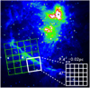 |
Fig. 1 Overlay of the PACS observations (CO J = 19–18) on a IRAC 8 μm image of the Orion Bar. A 4 × 4 raster map (16 overlapping footprints) is shown in green. A representation of a footprint with its 5 × 5 spatial pixels is illustrated in the bottom right corner of the figure together with their dimensions. |
2.2 Herschel/SPIRE
To complement the high-J CO PACS observations, we observed lower-J CO lines from J = 4−3 to J = 13−12, 13CO lines from J = 5−4 to J = 13−12, and C18O lines from J = 5−4 to J = 10−9. These observations were carried out in the high-resolution full-sampling mode of the SPIRE FTS instrument (Griffin et al. 2010) on March 20, 2010. We here highlight the comparison between the high-J CO (J = 19–18) and 13CO (J = 12−11) emission, but all the SPIRE CO, 13CO, and C18O lines show the same trends. These maps are first published in this paper and are presented in Appendix A.
The data were processed using HIPE 11.0.1. To achieve a better angular resolution, the super-resolution method SUPREME was applied to the FTS data as in Köhler et al. (2014). In the appendix (see Figs. A.1–A.3), we give an FWHM using a Gaussian fit with the same bandwidth of the equivalent beam. It should, however, be noted that the point spread function (PSF) is non-Gaussian and an FWHM does not account for the shape of the beam. The SUPREME method is based on the realistic physical model of the instrument and the regularized inversion. For a detailed description of the reduction procedure method, fitting routines, and PSF, see Ayasso et al. (2012) and the SUPREME web site2. With this method, we reach an angular resolution of 26′′ for CO J = 4–3 and 12′′ for CO and 13CO J =13–12 line. The spectra are not spectrally resolved (Δ λ∕λ ~ 315 km s−1 for CO J = 12-11). The lines were fitted with the HIPE Spectrometer Cube fitting procedure. We assume a conservative total error of 36−50% for the integrated line intensities from the combination of the calibration uncertainties (30%) and the line fitting errors (20−40%).
3 Spatial distribution of high-J CO emission
3.1 Morphology of the CO J = 19–18 emission
Figure 2 shows the map of the CO J = 19–18 integrated line intensity. The CO J = 19–18 line is detected unambiguously everywhere in the observed region (see Fig. 2).
The highest signal-to-noise ratio (~130σ) is reached in the Bar, as expected, but the detection is clear (σ ≥ 10) outside the Bar as well. Outside the Bar, the emission originates most likely also from the surface of the Orion molecular cloud-1 (OMC1). This surface is also illuminated by the Trapezium cluster, making it a face-on PDR. The high-J CO map shows and extended background emission in front of the Bar (closer to the ionizing stars) and behind the Bar. The emission from the background face-on PDR was also observed with Herschel in other PDR tracers, especially in [OI] 63 μm and to a lesser degree in [OI] 145 μm and [CII] 158 μm by Bernard-Salas et al. (2012). Closer to the Bar (both in front and behind), the emission increases gradually. The high-J CO line map also points to an increased emission at the western edge of the Bar. This excess was also detected in mid-J CO emission from the ground (e.g., Lis et al. 1998).
In the Bar, the most striking features are several knots of enhanced emission. These knots, one in the northeast, one in the center, and one in the southwest, are bridged by weaker emission. This morphology is somewhat mimicked in the OH and CH+ emissions (Parikka et al. 2017). The knot with maximum line intensity (4.75 × 10⁻⁴ erg s−1 cm−2 sr−1) is found in the northeastern part. Marginally resolved with diameters of about ~10−15′′, these knots may result in small-scale structures that we are not able to resolve. This is discussed in the following in a comparison with ground-based data (with ~1′′ of angular resolution) obtained with the ESO New Technology Telescope (NTT) and ALMA (see Sects. 3.2 and 5). Our observations can resolve structures of ~10′′. The substructures are probably surrounded by a lower-density gas, producing an extended interclump emission. Strong emission appears also to originate from the interclump regions of the Bar, although 55% of the emission originates from the emission knots (where the emission is >50% of the peak emission).
The FHWM of the high-J CO emission spatial profile toward the Bar is about ~15–20′′. As inferred in previous studies of PDRs surface tracers, this width is most likely the result of a projection effect along the line of sight and does not represent the physical thickness of high-J CO emission region. The Bar is tilted toward the observer (e.g., Hogerheijde et al. 1995; Allers et al. 2005; Pellegrini et al. 2009). To examine the effect of the inclination, we calculated the projected emission width considering that the high-J CO emission comes from the PDR edge with a density wall. Using an inclination angle of θ = 7° (Hogerheijde et al. 1995; Pellegrini et al. 2009) and a length of the PDR along the line of sight of 0.35 pc (Bernard-Salas et al. 2012) needed to reproduce the [CII] and [OI] emission, we find a projected emission width of sin(θ) × lPDR ~ 0.04 pc (or ~20′′). This projected width is in agreement with our derived FWHM mainly due to the inclination effect. The physical thickness of the high-J CO emission region must be much smaller.
 |
Fig. 2 Map of CO J = 19–18 integrated intensity. The contours are at levels of 0.3, 0.5, 0.7, and 0.9 of the peak emission. Beam size is indicated in the bottom left corner. The intensities are in units of erg s−1 cm−2 sr−1. |
3.2 Comparison with a tracer of the H/H2 transition
We compare the high-J CO emission to the vibrationally excited H2 emission, which originates from the thin PDR surface and delineates the H/H2 transition. The H2 v = 1−0 S(1) integrated intensity map with contours of CO J = 19–18 integrated intensity for the whole area where the high-J CO line was observed is plotted in Fig. 3. The H2 v = 1−0 S(1) was observed from the ground with a resolution of ~1′′ (Walmsley et al. 2000).
First, we find that the high-J CO emission peaks close to the peak of the H2 vibrational emission. A small shift (≲5′′) farther into the molecular cloud is generally observed for the CO emission. In specific places (i.e., in the center of the Bar, see Fig. 3), a spatial coincidence between the H2 1−0 S(1) and CO J = 19–18 peaks is observed. A shift between the two tracers is expected because CO is formed when H2 is self-shielded, that is, after the H/H2 transition. On the other hand, the small shift between the H2 and CO emission shows that the C+/C/CO transition may occur near the H/H2 transition. Much of the high-J CO emission must, in fact, originate after the H/H2 transition and at the C/CO transition before the gas temperature decreases. Our data cannot fully characterize the small shifts, but they are, however, in agreement with the recent work of Goicoechea et al. (2016) based on ALMA data, showing that there is no appreciable offset between the edge of the observed CO J = 3–2 and HCO+ J = 4–3 lines and the H2 vibrational emission. This is not expected in static equilibrium models of PDRs and is discussed in Sect. 5.
Second, Fig. 3 shows that the FWHM of the vibrationally emission H2 is about ~10′′, narrower than those observed for High-J CO. A similar FWHM is observed for the rotationally excited H2 emission (e.g., Allers et al. 2005). Furthermore, several substructures (with a typical width of 1−2′′) are observed in the H2 vibrational emission. High-J CO emission might originate from these substructures, but this cannot be determined from our data since these details are not resolved.
 |
Fig. 3 Map of H2 v = 1−0 S(1) integrated intensity (Walmsley et al. 2000) with overplotted contours of the CO J = 19–18 integrated intensity. The observations are not convolved, so that smaller structures are visible. The intensities are in units of erg s−1 cm−2 sr−1. |
3.3 Comparison with tracers of dense gas
In Fig. 4, we compare the CO J = 19–18 (137.3 μm) integrated intensity map to the 13CO J = 12−11 (209.5 μm) integrated intensity map. The CO J = 19–18 line is not convolved to the beam of the 13CO J = 12−11 line, but the angular resolutions of the two maps are similar, 9′′ for CO J = 19–18 emission and ~12′′ for 13CO J = 12−11 emission. The J = 19–18 line is shifted by ~5′′ relative to the 13CO line toward the ionizing stars. This is expected as the 13CO J =12−11 line comes from a lower energy transition and it will peak deeper in the Bar. On the other hand, the 12CO J = 12−11 line is not significantly shifted compared to the 13CO J = 12−11 (see Fig. A.1). The map of the 13CO J = 12−11 line also shows emission knots northeast and southwest of the Bar.
Another high-density tracer is the CS species. Lee et al. (2013) mapped the Orion Bar region in CS J =2−1 line, and two of the starless dense cores they mapped fall in the area we have observed. These condensations with a typical width of 5−10′′ have also been mapped by Lis & Schilke (2003) in H13CN, which is another dense core tracer. The emission knots in the 13CO J = 12−11 line appear to correlate with the dense cores as traced by H13 CN or CS (see Fig. 4 in this article and Fig. 4 in Lis & Schilke 2003). Lis & Schilke (2003) found cores 3 and 1 to correspond to knots of enhanced emission in the northeast and southwest part of the Bar. This is further evidence that the high-J CO emission is sensitive to higher column and/or volume density in this region. However, compared to the CO J = 19–18 emission, these cores and their fragments are located deeper inside the molecular cloud. The CO J = 19–18 emission is shifted ~5′′ toward the ionizing stars from the H13CN and CS J = 2−1 emission.
 |
Fig. 4 Map of the CO J = 19–18 integrated intensity. The contours of 13CO J = 12− 11 lie at levels of 0.5, 0.6, 0.7, 0.8, and 0.9 of the peak emission in the Bar. The intensities are given in units of erg s−1 cm−2 sr−1. |
4 High-JCO excitation
4.1 Spatial distribution of the CO J = 19–18 to CO J = 12–11 intensity ratio
To investigate the excitation of highly excited CO, we show in Fig. 5 the contour of the intensity ratio of CO J = 19–18 to CO J = 12–11 on top of CO J = 19–18 emission (left panel). In this figure, the CO J = 19–18 line has been convolved to the beam of the CO J = 12–11 line. This figure shows that the CO intensity ratio peaks in front of the CO J = 19–18 emission. The CO intensity ratio gradually decreases inside the Bar, but decreases faster in front of it. Behind the Bar, in the extended (background) emission the ratio is roughly constant and is lowest. In front of the Bar, the intensity ratio is somewhat high on the northwestern side, where the CO J = 12–11 (see Fig. A.1) and [OI] lines (see Fig. 2 of Bernard-Salas et al. 2012) are particularly low, while the high-J CO and [NII] 122 μm lines are not. The intensity of the high-J CO could indicate that the radiation field is higher. Alternatively, this might be due to variations in(column) density.
We also compare the intensity ratio of CO J = 19–18 to CO J = 12−11 lines with the Spitzer IRAC 8 μm (right panel), which traces the PAH emission. The left panel of Fig. 5 shows that PAH emission correlates well with the CO intensity ratio. Therefore, the CO ratio appears to peak between the H/H2 dissociation and the ionization fronts. This suggests the presence of a low column density hot molecular gas in the atomic region, where the intense UV radiation is mostly unshielded.
However, the face-on (OMC1) PDR emission could affect the interpretation of the edges of the maps. In order to confirm and quantify the properties of a warm or hot molecular gas in the atomic region, complementary data providing the spatial variation of the velocity line profile are needed.
Recent ALMA data revealed molecular gas between the ionization and dissociation fronts (Goicoechea et al. 2016). The data are consistent with photoevaporative neutral gas flows from the high-pressure molecular layers to the atomic layers. This is discussed in Sect. 5.
 |
Fig. 5 Contours of CO J = 19–18/CO J = 12–11 ratio overplotted on the CO J = 19–18 emission (left panel). The contours of CO J = 19–18/CO J = 12–11 intensity ratio overplotted on the IRAC 8 μm (right panel). The CO J = 19–18 line intensities are in units of erg s−1 cm−2 sr−1 and the 8 μm intensities are in units of MJy sr−1. The contours are separated by 1 and cover ratios from 1 to 5. |
4.2 Heating processes
In PDRs, heating results from impinging UV photons, but several different processes are involved to either directly or indirectly convert the energy input into kinetic energy (e.g., photoelectric effect, FUV H2 pumping). Given that PAHs dominate in part the photoelectric heating and correlate well with the excited CO ratio, it is likely that the photoelectric heating dominates the excitation of CO. We note, however, that the PAH emission peak is not the only indication of photoelectric heating, and photoelectric heating can therefore also dominate elsewhere.
For the physical conditions prevailing in the Orion Bar, the PDR Meudon model predicts that the photoelectric effect dominates throughout the high-J CO emission zone (Joblin et al. 2018). In the atomic layer of the high thermal pressure model by Joblin et al. (2018), FUV-pumped H2 followed by collisional deexcitation is an important heating process, but its rate is three times lower than the photoelectric heating rate. Only in very bright and dense PDRs can FUV-pumped H2 followed by collisional deexcitation dominate (e.g., Burton et al. 1990; Champion et al. 2017). In the successive layers, as soon as H2 is self-shielding, collisional deexcitation of H2 leads to cooling and the photoelectric heating dominates widely.
Therefore, all the CO emission originates from zones where the photoelectric effect dominates. The heating by formation of H2 never dominates and remains negligible compared to the photoelectric heating. Finally, we exclude the effect of cosmic rays, as we do not see an excitation effect beyond the diffuse region of the PDR.
4.3 Spectral distribution of all the observed CO and 13CO lines
In the following, we investigate the spectral line energy distribution (SLED) of all the observed lines of 12CO from J = 4−3 to J = 13−12 and J = 19–18 and 13CO from J = 5−4 to J = 13−12. The properties of these lines are summarized in Table 1. The integrated intensities of 12CO and 13CO observations convolved to26′′, the largest beam size (after SUPREME cube making) are shown in Fig. 6 for the three positions indicated in the map: in front of the Bar (blue), in the Bar (red), and behind the Bar (green). The positions in front and behind the Bar were chosen for agood signal-to-noise ratio for most of the lines. The three positions are spatially shifted by at least 26′′.
Figure 6 shows that the 12CO intensity is higher than the 13CO, as expected. The 12CO emission is optically thick in all the observed transitions, except for the J =19–18 transition (see the optical depth in Fig. 7). The 13CO is mostly optically thin. We examine the high-J CO to mid-J CO lines ratio in the three positions. High-J CO is a tracer of warm gas, with its higher upper level energy, while mid-J CO traces cooler gas. Thus, when the ratio is higher, the gas is warmer. Figure 6 shows that the temperature is highest in front of the Bar. The Bar is also warm, as the high-J and mid-J CO are comparable. Behind the Bar, the temperature is lower, but the gas is still warm. This is evidence of contribution from a warm background PDR, as has been discussed previously by Bernard-Salas et al. (2012). The derived temperature in the region is further discussed in Sect. 4.4 with the RADEX analysis.
Properties of the observed lines.
 |
Fig. 6 Integrated line intensity plotted against the upper level energy of the observed transitions. 12CO (circles) and 13CO (squares) in front of the Bar (blue), in the Bar (red), and behind the Bar (green), as indicated in the map. |
4.4 RADEX modeling
To assess the physical conditions in the Orion Bar, we analyzed the integrated intensities of 12CO and 13CO observations with RADEX3, a non-local thermal equilibrium (non-LTE) local radiative transfer code (van der Tak et al. 2007). By fitting RADEX models to observations, we can find solutions for the gas density, kinetic temperature, line optical depth, column density, and abundance of the species.
However, since RADEX assumes uniform temperature and density, we can only derive average physical conditions in the observed region. Assuming uniform density and temperature layer is very simplistic because different phases of gas are mixed along the line of sight and inside the Herschel beam area. The density and gas temperature could vary very rapidly throughout the PDR layer, and with our spatial resolution, the temperature structure is not spatially resolved. The high-J CO lines arise from a warmer layer with a lower column density than the intermediate-J CO lines. In Sect. 3, we find that the CO J = 19–18 and J = 12–11 emission peaks are shifted. Most of the CO J = 12–11 emission arises from a region that is colder than the PDR edge. Thus, the column density of the CO J = 12–11 is also expected to be significantly greater than the one derived from excited CO J = 19–18. Fitting all the lines with only one component is therefore an approximation, but it gives the average physical conditions of the emission zones in the Herschelbeam.
As in the previous section, we used the integrated intensities of 12CO and 13CO observations convolved to26′′, the largest beam size (after SUPREME cube making). This set of data (consistent beam size) ensures that we compare line intensities from the same area. The convolution can smooth the small areas of high-J CO line emission and can decrease their intensities.
We considered a grid of models and derived the kinetic temperature (Tg), CO column density (NCO), beam filling factor (η)4, thermal pressure (P), and length (l) along the line of sight. We considered gas densities nH 5 of 104 −107 cm−3, kinetic temperatures of 10−1000 K, CO column densities of 1015 −5 × 1019 cm−2, and the beam filling factor between 0.01 and 1. We used the new set of collisional rate coefficients, CO-H2, calculated by Yang et al. (2010), which includes energy levels up to J = 40 for temperatures ranging from 2 to 3000 K. We did not include CO-H collisions. We used a cosmic microwave background radiation temperature of 2.73 K and assumed a standard carbon isotopic ratio 12 C/13C of 70 (Wilson 1999). We also tested the model including intense FIR and submillimeter radiation emitted by dust with a temperatureof 40 and 80 K as the background source. We find that the effect of the dust continuum emission on the CO lines is negligible and has no effect on the fit. This suggests that FIR pumping does not affect the high-J CO population levels.
We used the observed data for the fitting procedure as follows: we fit the slope of the SLED of the CO lines with different combinations of kinetic temperature and gas density, which reflect a degeneracy between these two parameters. For a given combination of kinetic temperature and gas density, we obtained the CO column density, NCO, by fitting the CO to 13CO line ratio that is sensitive to the optical depth, which at the line center depends on the ratio of the column density to the line width. For reasons of simplicity, we assumed a constant width for all the lines measured in the FTS cubes. In addition, we assumed Δ v = 2.5 km s−1 (dense gas tracers with a line width of 2−3 km s−1 in the Orion Bar; Hogerheijde et al. 1995) and that the beam filling factor is constant for all of the lines. For each gas density, our fitting procedure yields the best fit corresponding to the minimum χ2. We also calculated the length along the line of sight, l, of the emission layer with  , where
  is the beam-averaged column density. In order to estimate l, we converted the CO into H2 column densities taking a relative CO abundance to H2 of 10−4.
In Fig. 7 we plot the results of the RADEX model at the peak of high-J CO flux emission, using all the observed transitions for 12CO and 13CO. We plot the integrated line intensities against the upper energy levels of the transitions. The observations are plotted in black and the fits for different hydrogen densities, nH: 105, 106, and 107 cm−3, are plotted in colored lines, red, green, and blue, respectively. The results for the fits with different gas densities in this position are shown in Table 2.
Our best fit is obtained for a density of nH ~106 cm−3 and a temperature of Tg ~160 K. The derived thermal pressure is high, about P ~ 1−2 × 10⁸ K cm−3. The derived length along the line of sight is l ~ 0.026 pc (or 13′′). Consideringthat the excited CO comes from the surface of the Bar tilted by θ = 7°, l can be given by l= e∕sin(θ) with e being the physical thickness. This thickness should be small since the excited CO traces the thin PDR surface. Taking l ~ 0.026 pc, we find e ~ 0.003 pc or ~1′′. This is in agreement with PDR models for gas at high-pressure (e.g., Allers et al. 2005; Bron et al. 2018; Joblin et al. 2018). For a density of 105 cm−3, l is much too long (230′′), since n is small and it does not match the geometrical view of the Orion Bar.
The beam filling factor, η, is found to be ~0.4. This implies that the warm CO emission on average covers 40% of the Herschel SPIRE beams (~25′′). The derived warm CO column density is NCO ~ 4 × 1018 cm−2, corresponding to an hydrogen column density of  . This represents about 40% of the total column along the line of sight (~2 × 1023 cm−2; Johnstone et al. 2003). We discuss the results in more detail and in comparison to previous research in Sect. 5.
 |
Fig. 7 Top panel: integrated line intensities of 12CO observationsfrom J = 5−4 to J = 13−12 and J = 19–18 (black squares) and 13CO observationsfrom J = 5−4 to J = 13−12 (black triangles) are plotted against the upper energy levels of the transitions. The colored lines are the different RADEX fits for different hydrogen densities (nH): 105 (red), 106 (blue), and 107 (green).The results of the fits are shown in Table 2. Bottom panels: optical depth plotted against the upper level energy for the best fits for each hydrogen density show in the top figure. |
Results for RADEX modeling for the selected position in the Bar.
5 Discussion
5.1 Inhomogeneous clumpy structure and physical conditions
In bright PDRs, such as the Orion Bar, uniform models have been proven insufficient to model the observations. These models have suggested that dense components are embedded in lower density gas that have not been resolved by observations (e.g., Stutzki & Guesten 1990; Tauber et al. 1994). In particular, the high-J CO rotational line (J = 14−13), observed from the ground (Tauber et al. 1994), seems to arise in dense small-scale structures in PDR surface, while the C+ emission is dominated by the surrounding medium with lower density. Clumpy models have also been suggested. Burton et al. (1990) modeled H2 and CO molecules with a clumpy model. They found that the CO emission in the Orion Bar comes from high-density clumps of 106−7 cm−3 and also from an interclump medium of 104−5 cm−3. In addition, Young Owl et al. (2000) found that a clumpy model can explain their observations of HCO+ and HCN. They found a dense clump density of 3 × 106 cm−3 and an interclump medium density of 5 × 104 cm−3. Recently, Andree-Labsch et al. (2017) have produced similar results with their 3D model. This modeling resulted in dense clumps of 4 × 106 cm−3 and in an interclump medium density of 105 cm−3.
Our derived density and thermal pressure are comparable to previous studies of the Orion Bar (e.g., Goicoechea et al. 2016; Andree-Labsch et al. 2017; Nagy et al. 2017). Goicoechea et al. (2016) and Nagy et al. (2017) found gas densities of 105 –106 cm−3 and a pressure of P ~ 2 × 10⁸ K cm−3. The density is about ten times lower than the density derived from colder density tracers such as CS (Lee et al. 2013).
Arab et al. (2012) fit the observed dust emission stratification toward the Bar. Using the DustEM model, they found a temperature of 50 K, a gas density of 1.5 × 105 cm−3, and a length of 0.45 pc in the Bar. We find a higher gas density (106 cm−3) to fit the high-J CO. Our results do not necessarily contradict the results of Arab et al. (2012). The difference might be due to the bulk of the dust originating in a lower density medium. Cores and their fragments are typically higher density concentrations embedded in a larger filamentary structure at a lower density. The 3D model of Andree-Labsch et al. (2017) found similar results to ours with a clump density of 4 × 106 cm−3 and an interclump medium of ×105 cm−3. This model used ensemble-averaged densities, and the density can also be higher locally.
5.2 Fragmented molecular edge
ALMA observations resolve (with ~1′′ of angular resolution) the sharp molecular edge where the CO J = 3–2 and HCO+ J = 4−3 line emissions become intense (Goicoechea et al. 2016). These observations show a detailed morphology of the PDR irregular illuminated surface. They find a fragmented molecular edge of high-density substructures (filamentary substructures, some similar to globulettes, with a typical width of about 2′′) surrounding the H/H2 dissociation front and roughly parallel to it. This morphology of the Bar is not resolved with the 9′′ resolution of Herschel. This is in agreement with the knots of enhanced emission we detect in the Bar, however, and even smaller than we can see in the CO J = 19–18 line emission map.
The sharp edge coincides with the brightest peaks of the H2 v = 1−0 S(1) vibrational emission tracing the H/H2 transition (extended data Fig. 2, Goicoechea et al. 2016) and shows that the H/H2 and the C+/C/CO transition zones occur very close to each other. This is also in agreement with our comparison of the CO J = 19–18 line with the H2 vibrational emission. This result is not expected by PDR static equilibrium models, where the C/CO transition must occur deeper inside. This suggests that dynamical effects are important. The cloud edge could have been compressed by a high-pressure wave that is moving into the molecular cloud (Goicoechea et al. 2016; Bron et al. 2018).
5.3 Molecular gas between the ionization and dissociation fronts
ALMA reveals fainter HCO+ J = 4−3 and CO J = 3–2 emission in the atomic layer (Goicoechea et al. 2016). Moreover, molecular line profiles show two velocity components, one corresponding to the gas from inside the Orion Bar, and another from the background molecular cloud. The velocity dispersion shows its maximum between the ionization and the dissociation fronts.
Both the kinematic association with the Orion Bar velocities and the higher velocity dispersion between the two fronts are consistent with the presence of gas flowing from the high-pressure compressed molecular layers (P ~ 2 × 10⁸ K cm−3) to the atomic layers (P ~ 5 × 10⁷ K cm−3). This is in agreement with our derived thermal pressure in the CO emitting layers and the CO J = 19–18 to J = 12–11 line ratio map, which suggests a low column density of hot molecular gas in the atomic layer.
6 Conclusions and summary
We presented for the first time high spatial resolution images of rotationally excited CO over a large area of ~110′′× 110′′ using Herschel. We find a clear detection of CO J = 19–18 over the whole region. In the Bar, the most striking features are several knots of enhanced emission. The CO J = 19–18 emission peaks are close to the brightest peaks of the H2 vibrational emission, which suggests that the H/H2 and the C+/C/CO transition zones occur very close to each other, in agreement with recent ALMA studies. Our results also suggest that the warm and hot CO is mainly heated by the photoelectric effect on grains and PAHs. A low column density of warm and hot molecular gas could be present in the atomic layer. This is also in agreement with recent ALMA observations (Goicoechea et al. 2016) and hydrodynamical PDR simulations (Bron et al. 2018), which suggest that the dynamical effects are important.
We used RADEX models to analyze the spectral distribution of all the observed CO and 13CO transitions and to derive the hydrogen density, 12CO column density, temperature, and thermal pressure. The high-J CO intensity is very sensitive to the pressure. The RADEX modeling gives several solutions; the best fit has a density of 106 cm−3 and a thermal pressure of ~2 × 10⁸ K cm−3. This is comparable to other studies of the Orion Bar (e.g., Goicoechea et al. 2016; Andree-Labsch et al. 2017; Nagy et al. 2017) and consistent with gas flowing from the high-pressure molecular layers to the atomic layers. Finally, we showed that the emission of 13CO J = 12−11 is associated with the dense core of the clumps, as traced by CS (Lee et al. 2013) and H13CN (Lis & Schilke 2003).
Acknowledgements
J.B.-S. wishes to acknowledge the support of a Career Integration Grant within the 7th European Community Framework Program, FP7-PEOPLE-2013-CIG-630861-FEASTFUL.
Appendix A Orion Bar maps in 12CO, 13CO, and C18O
In Fig. A.1 we present the 12CO maps lines from J = 4−3 to J = 13−12. Maps of 13CO lines from J = 5−4 to J =13−12 are shown in Fig. A.2 and C18O lines from J = 5−4 to J = 13−12 are shown in Fig. A.3. All maps are projected to the area of 12CO J =19–18 map, and the beam size from the Supreme reduction is shown in the bottom left corner.
 |
Fig. A.1 12CO SPIRE maps. The beam size is indicated in the bottom left corner. |
 |
Fig. A.2 13CO SPIRE maps. The beam size is indicated in the bottom left corner. |
 |
Fig. A.3 C18O SPIRE maps. The beam size is indicated in the bottom left corner. |
We stress that the PSF of the CO J = 19–18 and J = 12−11 lines observed with PACS and SPIRE, respectively, differs significantly in the wings. This could induce some artificial effects in the intensity ratio (shown in Fig. 5), particularly at the edge of the emission profiles, that is, at the edge of Bar.
References
- Allers, K. N., Jaffe, D. T., Lacy, J. H., Draine, B. T., & Richter, M. J. 2005, ApJ, 630, 368 [NASA ADS] [CrossRef] [Google Scholar]
- Andree-Labsch, S., Ossenkopf-Okada, V., & Röllig, M. 2017, A&A, 598, A2 [NASA ADS] [CrossRef] [EDP Sciences] [Google Scholar]
- Arab, H., Abergel, A., Habart, E., et al. 2012, A&A, 541, A19 [NASA ADS] [CrossRef] [EDP Sciences] [Google Scholar]
- Ayasso, H., Rodet, T., & Abergel, A. 2012, Inverse Problems, 28, 125005 [Google Scholar]
- Bernard-Salas, J., Habart, E., Arab, H., et al. 2012, A&A, 538, A37 [NASA ADS] [CrossRef] [EDP Sciences] [Google Scholar]
- Bron, E., Agúndez, M., Goicoechea, J. R., & Cernicharo, J. 2018, A&A, submitted [arXiv:1801.01547] [Google Scholar]
- Burton, W. B., & Gordon, M. A. 1978, A&A, 63, 7 [NASA ADS] [Google Scholar]
- Burton, W. B., Gordon, M. A., Bania, T. M., & Lockman, F. J. 1975, ApJ, 202, 30 [NASA ADS] [CrossRef] [Google Scholar]
- Burton, M. G., Hollenbach, D. J., & Tielens, A. G. G. M. 1990, ApJ, 365, 620 [NASA ADS] [CrossRef] [Google Scholar]
- Cazzoli, G., Puzzarini, C., & Lapinov, A. V. 2004, ApJ, 611, 615 [NASA ADS] [CrossRef] [Google Scholar]
- Champion, J., Berné, O., Vicente, S., et al. 2017, A&A, 604, A69 [NASA ADS] [CrossRef] [EDP Sciences] [Google Scholar]
- Dame, T. M., & Thaddeus, P. 1985, ApJ, 297, 751 [NASA ADS] [CrossRef] [Google Scholar]
- Dame, T. M., Ungerechts, H., Cohen, R. S., et al. 1987, ApJ, 322, 706 [NASA ADS] [CrossRef] [Google Scholar]
- Flower, D. R. 2001, J. Phys. B At. Mol. Phys., 34, 2731 [NASA ADS] [CrossRef] [Google Scholar]
- Furukawa, N., Ohama, A., Fukuda, T., et al. 2014, ApJ, 781, 70 [NASA ADS] [CrossRef] [Google Scholar]
- Godard, B., & Cernicharo, J. 2013, A&A, 550, A8 [NASA ADS] [CrossRef] [EDP Sciences] [Google Scholar]
- Goicoechea, J. R., Chavarría, L., Cernicharo, J., et al. 2015, ApJ, 799, 102 [NASA ADS] [CrossRef] [Google Scholar]
- Goicoechea, J. R., Pety, J., Cuadrado, S., et al. 2016, Nature, 537, 207 [NASA ADS] [CrossRef] [Google Scholar]
- Griffin, M. J., Abergel, A., Abreu, A., et al. 2010, A&A, 518, L3 [Google Scholar]
- Hogerheijde, M. R., Jansen, D. J., & van Dishoeck E. F. 1995, A&A, 294, 792 [NASA ADS] [Google Scholar]
- Indriolo, N., Bergin, E. A., Goicoechea, J. R., et al. 2017, ApJ, 836, 117 [NASA ADS] [CrossRef] [Google Scholar]
- Joblin, C., Bron, E., Pinto, C., et al. 2018, A&A, 615, A129 [NASA ADS] [CrossRef] [EDP Sciences] [Google Scholar]
- Johnstone, D., Boonman, A. M. S., & van Dishoeck E. F. 2003, A&A, 412, 157 [NASA ADS] [CrossRef] [EDP Sciences] [Google Scholar]
- Karska, A., Herpin, F., Bruderer, S., et al. 2014, A&A, 562, A45 [NASA ADS] [CrossRef] [EDP Sciences] [Google Scholar]
- Kazandjian, M. V., Meijerink, R., Pelupessy, I., Israel, F. P., & Spaans, M. 2012, A&A, 542, A65 [NASA ADS] [CrossRef] [EDP Sciences] [Google Scholar]
- Kazandjian, M. V., Meijerink, R., Pelupessy, I., Israel, F. P., & Spaans, M. 2015, A&A, 574, A127 [NASA ADS] [CrossRef] [EDP Sciences] [Google Scholar]
- Köhler, M., Habart, E., Arab, H., et al. 2014, A&A, 569, A109 [NASA ADS] [CrossRef] [EDP Sciences] [Google Scholar]
- Lebouteiller, V., Cormier, D., Madden, S. C., et al. 2012, A&A, 548, A91 [NASA ADS] [CrossRef] [EDP Sciences] [Google Scholar]
- Lee, K., Looney, L. W., Schnee, S., & Li, Z.-Y. 2013, ApJ, 772, 100 [NASA ADS] [CrossRef] [Google Scholar]
- Lis, D. C., & Schilke, P. 2003, ApJ, 597, L145 [NASA ADS] [CrossRef] [Google Scholar]
- Lis, D. C., Serabyn, E., Keene, J., et al. 1998, ApJ, 509, 299 [Google Scholar]
- Marconi, A., Testi, L., Natta, A., & Walmsley, C. M. 1998, A&A, 330, 696 [NASA ADS] [Google Scholar]
- Martín, S., Martín-Pintado, J., & Viti, S. 2009, ApJ, 706, 1323 [NASA ADS] [CrossRef] [Google Scholar]
- Meijerink, R., Spaans, M., & Israel, F. P. 2007, A&A, 461, 793 [NASA ADS] [CrossRef] [EDP Sciences] [Google Scholar]
- Menten, K. M., Reid, M. J., Forbrich, J., & Brunthaler, A. 2007, A&A, 474, 515 [NASA ADS] [CrossRef] [EDP Sciences] [Google Scholar]
- Nagy, Z., Choi, Y., Ossenkopf-Okada, V., et al. 2017, A&A, 599, A22 [NASA ADS] [CrossRef] [EDP Sciences] [Google Scholar]
- O’Neil, K., Hofner, P., & Schinnerer, E. 2000, ApJ, 545, L99 [NASA ADS] [CrossRef] [Google Scholar]
- Papadopoulos,P. P., Isaak, K., & van der Werf, P. 2010, ApJ, 711, 757 [NASA ADS] [CrossRef] [Google Scholar]
- Parikka, A., Habart, E., Bernard-Salas, J., et al. 2017, A&A, 599, A20 [NASA ADS] [CrossRef] [EDP Sciences] [Google Scholar]
- Pellegrini, E. W., Baldwin, J. A., Ferland, G. J., Shaw, G., & Heathcote, S. 2009, ApJ, 693, 285 [NASA ADS] [CrossRef] [Google Scholar]
- Poglitsch, A., Waelkens, C., Geis, N., et al. 2010, A&A, 518, L2 [NASA ADS] [CrossRef] [EDP Sciences] [Google Scholar]
- Schleicher, D. R. G., Spaans, M., & Klessen, R. S. 2010, A&A, 513, A7 [NASA ADS] [CrossRef] [EDP Sciences] [Google Scholar]
- Schwartz, P. R., Wilson, W. J., & Epstein, E. E. 1973, ApJ, 186, 529 [NASA ADS] [CrossRef] [Google Scholar]
- Scoville, N. Z., & Solomon, P. M. 1975, ApJ, 199, L105 [NASA ADS] [CrossRef] [Google Scholar]
- Solomon, P. M., Rivolo, A. R., Barrett, J., & Yahil, A. 1987, ApJ, 319, 730 [NASA ADS] [CrossRef] [Google Scholar]
- Sturm, B., Bouwman, J., Henning, T., et al. 2010, A&A, 518, L129 [NASA ADS] [CrossRef] [EDP Sciences] [Google Scholar]
- Stutzki, J., & Guesten, R. 1990, ApJ, 356, 513 [NASA ADS] [CrossRef] [Google Scholar]
- Tauber, J. A., Tielens, A. G. G. M., Meixner, M., & Foldsmith, P. F. 1994, ApJ, 422, 136 [NASA ADS] [CrossRef] [Google Scholar]
- Tielens, A. G. G. M., & Hollenbach, D. 1985, ApJ, 291, 747 [NASA ADS] [CrossRef] [Google Scholar]
- Tielens, A. G. G. M., Meixner, M. M., van der Werf, P. P., et al. 1993, Science, 262, 86 [NASA ADS] [CrossRef] [PubMed] [Google Scholar]
- van der Tak, F. F. S., Black, J. H., Schöier, F. L., Jansen, D. J., & van Dishoeck, E. F. 2007, A&A, 468, 627 [NASA ADS] [CrossRef] [EDP Sciences] [Google Scholar]
- Visser, R., Kristensen, L. E., Bruderer, S., et al. 2012, A&A, 537, A55 [NASA ADS] [CrossRef] [EDP Sciences] [Google Scholar]
- Walmsley, C. M., Natta, A., Oliva, E., & Testi, L. 2000, A&A, 364, 301 [NASA ADS] [Google Scholar]
- Wilson, T. L. 1999, Rep. Prog. Phys., 62, 143 [Google Scholar]
- Wilson, R. W., Jefferts, K. B., & Penzias, A. A. 1970, ApJ, 161, L43 [NASA ADS] [CrossRef] [Google Scholar]
- Winnewisser, G., Belov, S. P., Klaus, T., & Schieder, R. 1997, J. Mol. Spectr., 184, 468 [NASA ADS] [CrossRef] [Google Scholar]
- Yang, B., Stancil, P. C., Balakrishnan, N., & Forrey, R. C. 2010, ApJ, 718, 1062 [NASA ADS] [CrossRef] [Google Scholar]
- Young Owl, R. C., Meixner, M. M., Wolfire, M., Tielens, A. G. G. M., & Tauber, J. 2000, ApJ, 540, 886 [NASA ADS] [CrossRef] [Google Scholar]
From the PACS spectroscopy performance and calibration manual. This can be found at http://herschel.esac.esa.int/twiki/bin/view/Public/PacsCalibrationWeb.
The beam filling factor, η, is the ratio between the line emission area and the beam area.
The input parameter for RADEX is  , and we consider
  .
.
All Tables
All Figures
|
Fig. 1 Overlay of the PACS observations (CO J = 19–18) on a IRAC 8 μm image of the Orion Bar. A 4 × 4 raster map (16 overlapping footprints) is shown in green. A representation of a footprint with its 5 × 5 spatial pixels is illustrated in the bottom right corner of the figure together with their dimensions. |
| In the text | |
|
Fig. 2 Map of CO J = 19–18 integrated intensity. The contours are at levels of 0.3, 0.5, 0.7, and 0.9 of the peak emission. Beam size is indicated in the bottom left corner. The intensities are in units of erg s−1 cm−2 sr−1. |
| In the text | |
|
Fig. 3 Map of H2 v = 1−0 S(1) integrated intensity (Walmsley et al. 2000) with overplotted contours of the CO J = 19–18 integrated intensity. The observations are not convolved, so that smaller structures are visible. The intensities are in units of erg s−1 cm−2 sr−1. |
| In the text | |
|
Fig. 4 Map of the CO J = 19–18 integrated intensity. The contours of 13CO J = 12− 11 lie at levels of 0.5, 0.6, 0.7, 0.8, and 0.9 of the peak emission in the Bar. The intensities are given in units of erg s−1 cm−2 sr−1. |
| In the text | |
|
Fig. 5 Contours of CO J = 19–18/CO J = 12–11 ratio overplotted on the CO J = 19–18 emission (left panel). The contours of CO J = 19–18/CO J = 12–11 intensity ratio overplotted on the IRAC 8 μm (right panel). The CO J = 19–18 line intensities are in units of erg s−1 cm−2 sr−1 and the 8 μm intensities are in units of MJy sr−1. The contours are separated by 1 and cover ratios from 1 to 5. |
| In the text | |
|
Fig. 6 Integrated line intensity plotted against the upper level energy of the observed transitions. 12CO (circles) and 13CO (squares) in front of the Bar (blue), in the Bar (red), and behind the Bar (green), as indicated in the map. |
| In the text | |
|
Fig. 7 Top panel: integrated line intensities of 12CO observationsfrom J = 5−4 to J = 13−12 and J = 19–18 (black squares) and 13CO observationsfrom J = 5−4 to J = 13−12 (black triangles) are plotted against the upper energy levels of the transitions. The colored lines are the different RADEX fits for different hydrogen densities (nH): 105 (red), 106 (blue), and 107 (green).The results of the fits are shown in Table 2. Bottom panels: optical depth plotted against the upper level energy for the best fits for each hydrogen density show in the top figure. |
| In the text | |
|
Fig. A.1 12CO SPIRE maps. The beam size is indicated in the bottom left corner. |
| In the text | |
|
Fig. A.2 13CO SPIRE maps. The beam size is indicated in the bottom left corner. |
| In the text | |
|
Fig. A.3 C18O SPIRE maps. The beam size is indicated in the bottom left corner. |
| In the text | |
Current usage metrics show cumulative count of Article Views (full-text article views including HTML views, PDF and ePub downloads, according to the available data) and Abstracts Views on Vision4Press platform.
Data correspond to usage on the plateform after 2015. The current usage metrics is available 48-96 hours after online publication and is updated daily on week days.
Initial download of the metrics may take a while.