| Issue |
A&A
Volume 617, September 2018
|
|
|---|---|---|
| Article Number | A31 | |
| Number of page(s) | 16 | |
| Section | Interstellar and circumstellar matter | |
| DOI | https://doi.org/10.1051/0004-6361/201731658 | |
| Published online | 12 September 2018 | |
Revisiting the case of R Monocerotis: Is CO removed at R < 20 au?★
1
Observatorio Astronómico Nacional (IGN),
Calle Alfonso XII 3,
28014
Madrid,
Spain
e-mail: This email address is being protected from spambots. You need JavaScript enabled to view it.
, This email address is being protected from spambots. You need JavaScript enabled to view it.
2
Instituto de Ciencia de Materiales de Madrid (ICMM-CSIC),
28049
Cantoblanco,
Madrid,
Spain
e-mail: This email address is being protected from spambots. You need JavaScript enabled to view it.
3
Departamento de Astrofísica, Centro de Astrobiología (CAB, CSIC-INTA), ESAC Campus, Camino Bajo del Castillo s/n, Villanueva de la Cañada,
28692
Madrid,
Spain
4
Chalmers University of Technology, Onsala Space Observatory,
439 92
Onsala,
Sweden
Received:
27
July
2017
Accepted:
20
May
2018
Abstract
Context. To our knowledge, R Mon is the only B0 star in which a gaseous Keplerian disk has been detected. However, there is some controversy about the spectral type of R Mon. Some authors propose that it could be a later B8e star, where disks are more common.
Aims. Our goal is to re-evaluate the R Mon spectral type and characterize its protoplanetary disk.
Methods. The spectral type of R Mon has been re-evaluated using the available continuum data and UVES emission lines. We used a power-law disk model to fit previous 12CO 1 →0 and 2 →1 interferometric observations and the PACS CO data to investigate the disk structure. Interferometric detections of 13CO J = 1 →0, HCO+ 1 →0, and CN 1 →0 lines using the IRAM Plateau de Bure Interferometer (PdBI) are presented. The HCN 1 →0 line was not detected.
Results. Our analysis confirms that R Mon is a B0 star. The disk model compatible with the 12CO 1 →0 and 2 →1 interferometric observations falls short of predicting the observed fluxes of the 14 < Ju < 31 PACS lines; this is consistent with the scenario in which some contribution to these lines is coming from a warm envelope and/or UV-illuminated outflow walls. More interestingly, the upper limits to the fluxes of the Ju > 31 CO lines suggest the existence of a region empty of CO at R ≲ 20 au in the protoplanetary disk. The intense emission of the HCO+ and CN lines shows the strong influence of UV photons on gas chemistry.
Conclusions. The observations gathered in this paper are consistent with the presence of a transition disk with a cavity of Rin ≳ 20 au around R Mon. This size is similar to the photoevaporation radius that supports the interpretation that UV photoevaporation is main disk dispersal mechanism in massive stars
Key words: circumstellar matter / stars: emission-line, Be / stars: formation
The reduced PdBI datacubes are only available at the CDS via anonymous ftp to cdsarc.u-strasbg.fr (130.79.128.5) or via http://cdsarc.u-strasbg.fr/viz-bin/qcat?J/A+A/617/A31
© ESO 2018
1 Introduction
Herbig Ae/Be stars are intermediate mass (M ~ 2−8 M⊙) pre-main sequence objects. These objects share many characteristics with high-mass stars such as clustering and the existence of photodissociation regions (PDRs) in their surroundings, but their study presents an important advantage: there are many located closer to the Sun (d ≤ 1 Kpc) and in regions less complex than massive star forming regions. The detection and detailed study of circumstellar disks around Herbig Ae/Be stars could provide valuable information to understand the formation of massive stars.
In recent years, there has been much theoretical and observational work with the aim of understanding disk occurrence and evolution in Herbig Ae/Be stars. Similar to the case of their low-mass counterpart T Tauri stars (TTs), the spectral energy distribution (SED) of many of these stars is characterized by an infrared excess due to thermal emission of circumstellar dust. But the exact geometry of this circumstellar dust (disk, disk+shell, shell) is not clear. It is generally accepted that disks similar to those associated with TTs surround Herbig Ae and late-type Be stars (Alonso-Albi et al. 2009; Boissier et al. 2011), but their existence around more massive Be stars (spectral type earlier than B6) is uncertain. Evidence of the existence of dusty and gaseous disks around some Herbig Be stars exist at optical, near-infrared (NIR), and mid-IR wavelengths (Meeus et al. 2001; Millan-Gabet et al. 2001; Vink et al. 2002; Acke et al. 2005), but the direct detection of the disks at millimeter wavelengths remains elusive with only a handful of detections (Alonso-Albi et al. 2009). Since the disk is optically thick at NIR and mid-IR wavelengths, millimeter observations are required to estimate the dust and gas mass in the disk. On the other hand, spectroscopic observations of molecular lines are useful to study the disk dynamics.
Observations of disks have been carried out using the Photoconductor Array Camera and Spectrometer (PACS) instrument onboard the Herschel Space Observatory (HSO), within the Key Programs Dust, Ice, and Gas In Time (DIGIT; Green et al. 2013) and Gas in Protoplanetary Systems (GASPS; Dent et al. 2013).These observations report the detection of pure rotational high-J (Ju > 14) CO emission lines in these sources (e.g., Sturm et al. 2010; van Kempen et al. 2010; Meeus et al. 2012, 2013). Thermochemical models of UV irradiated disks show that these lines are tracing the warm gas (Tk > 300 K) located in intermediate layers between the disk surface and the midplane at intermediate distances from the star (10–50 au) (e.g., Jonkheid et al. 2007; Gorti & Hollenbach 2008; Woitke et al. 2009; Kamp et al. 2010; Bruderer et al. 2012; Fedele et al. 2013). However, the PACS spectra are spectrally and spatially unresolved and their comparison with models involves some ambiguity. The detected high-J CO emission could arise in the hot inner envelopes and/or molecular outflows associated with these young stars instead of in the UV-irradiated disk. Fedele et al. (2013) derived, for the first time, the radial gas temperature gradient in the disk associated with the Herbig Ae star HD 100546 based on the combination of data from PACS and spectrally resolved CO spectra from the Heterodyne Instrument for the Far-Infrared (HIFI) onboard the HSO. In Fedele et al. (2016), this kind of study was extended to HD 97048, AS 205, Oph-IRS 2-48, S CrA, TW Hya, HD 100546, and HD 163296.
R Mon is a very young Herbig Be star located at a distance of 800 pc (Cohen et al. 1985). It is associated with the reflection nebula NGC 2261 and has a T Tauri companion located 0.7′′ NW (Close et al. 1997). The star drives a prominent molecular outflow that excites the HH 39 object, located in a small dark cloud 7′ N from R Mon (Canto et al. 1981; Jones & Herbig 1982; Brugel et al. 1984). Based on continuum interferometric observations, Fuente et al. (2003) detected a ~0.01 M⊙ circumstellar disk toward R Mon. Subsequent interferometric observations of the CO 1 →0 and 2 →1 molecular lines showed the existence of a large gaseous disk in Keplerian rotation around the star (Fuente et al. 2006). Alonso-Albi et al. (2009) carried out a complete modeling of the SED including interferometric measurements at millimeter and centimeter wavelengths. They derived a more accurate value of the dust mass (1.4× 10⁻⁴ M⊙) and showed that grain growth has proceeded to sizes of ~1 cm in the disk midplane. In addition to the compact disk (Rin = 18 au, Rout = 150 ± 50 au), a toroidal envelope of ~0.8 M⊙ (Rin = 700 au, Rout = 12 000 au) was needed to fit the single-dish far-infrared (FIR) fluxes (Alonso-Albi et al. 2009).
Some controversy exists about the spectral type of R Mon, which is crucial for the correct interpretation of the existing data. Early studies by The et al. (1994) classified R Mon as a B0 star. Close et al. (1997) also classified this object as B0 after a detailed discussion of the available photometry, extinction, and estimated bolometric luminosity. Later, Mora et al. (2001) classified R Mon as a B8 III, which is consistent with a luminosity of ~450 L⊙ derived by Natta et al. (1993). Fuente et al. (2006) determined that the mass of the star is 8 ± 1 M⊙ based on the Keplerian disk rotation, which is consistent with a young B0 star. However, Sandell et al. (2011) suggested that the rotation curve could be contaminated by the outflow emission and R Mon could rather be a late-type Be star in which circumstellar disks are common. In order to interpret the millimeter and infrared data, a critical revision of the spectral type is necessary. If confirmed, R Mon would be one of the closest B0 stars and the only one with a disk detected in molecular lines.
In this paper, we present new interferometric detections of the 13CO 1 →0, CN 1 →0, and HCO+ 1 →0 lines towardR Mon. We revise the stellar spectral type to determine the disk parameters taking advantage of the current available (PACS, interferometric) data. In more detail, in Sect. 4 we redo the determination of the R Mon spectral type using the stellar SED and high-resolution spectroscopy in ultraviolet (UV) wavelengths. In Sect. 5 we investigate its physical structure based on the Herschel/PACS observations of the high-J CO lines combined with our interferometric CO 1 →0 and 2 →1 observations. Finally, we compare the new 13CO 1 →0, CN 1→0 and HCO+ 1 →0 lines with our model in Sect. 7.
2 Data acquisition
2.1 UVES/VLT spectrum
We have used an archival spectrum from the UV and Visual Echelle Spectrograph (UVES) at Very Large Telescope (VLT), obtained on March 16, 2009. The data correspond to the reduced products provided by the ESO archive. Although the two arms of UVES spectrograph overlap, the usable data available have a gap of ~4980–5680 Å.
2.2 Herschel - PACS
R Mon was observed by the HSO in PACS range spectroscopic mode during September 2016, as part of the proposal OT1_gmeeus_1. The wavelength range of ~50–190 μm was covered by two different observations, with OBSID 1342250902 and 1342250903 (see Fig. 1). The observations were performed in the pointed chop-nod mode to be able to subtract the telescope and background contributions. A small chopper throw (1.5′′) was used, aiming to minimize the effect of field rotation between the two chop positions. Only one nodding cycle was performed for a total exposure time of 2240 s. The observations were reduced using HIPE 15, with the standard routine for chopped observations and the version 78 of the tree calibration files. In Tables 1 and A.1 we show the integrated line fluxes of the lines detected with PACS. Line fluxes were extracted from the central spatial pixel (spaxel) of the spectrometer, and aperture corrected to account for flux loss in the surrounding spaxels.
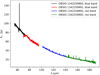 |
Fig. 1 PACS spectroscopic observations from 50 to 190 μm, showing the prominent [OI] emission at 63 μm as well as the CO lines. |
2.3 Plateau de Bure Interferometer (PdBI)
Interferometric observations of the 13CO 1 →0 and 2 →1 lines were carried out in January 2006 within project P055. By that time the configuration of the receivers of the PdBIallowed us to observe the 3 mm and 1 mm bands simultaneously. The observations were performed in A configuration and six antennas. Correlator units of 80 MHz providing a spectral resolution of ~78 kHz were used for the spectral observations of the 13CO 1 →0 and 2 →1 lines. The 13CO 1 →0 line was detected with a S/N ratio of ~5 (integrated intensity). The 13CO 2 →1 line was not detected down to an rms of 12.0 mJy beam−1 in 1 km s−1 channel.
The interferometric observations of CN, HCN, and HCO+ were carriedout in September (configuration D) and December 2008 (configuration C; project S01A). The 80 MHz correlator unit was placed at 113.490 GHz providing a spectral resolution of 78 kHz to cover the most intense hyperfine components of the CN 1 →0 line. The HCO+ 1 →0 and HCN 1 →0 lines were observed simultaneously with the receiver centered at the frequency of 88.910 GHz. During the observations, two 40 MHz bandwidth correlator units were placed at the frequency of the HCN 1 →0 and HCO+ 1 →0 lines, respectively, providing a spectral resolution of ~39 kHz (0.13 km s−1). To improve the S/N ratio we degraded the velocity resolution of the HCO+ and HCN lines to 0.3 km s−1. The HCN 1 →0 line was not detected with a final rms of ~5 mJy beam−1 in a channel of 0.3 km s−1.
Data reduction and image synthesis were carried out using the GILDAS1 software. The channels free of line emission were used to estimate the continuum flux that was subtracted from the spectral maps. The main observational parameters are listed in Table 2.
3 Observational results
3.1 PACS fluxes
A variety of CO, H2O, and OI emission lines were detected in the 50–200 μm range. For the detected lines, we computed line fluxes by fitting a Gaussian profile to the continuum subtracted spectra in a region 1 μm wide aroundeach feature. The line flux uncertainties were estimated as a Gaussian integral with a peak equal to the noise of the continuum in the region of interest, and a width equal to the fitted value. For nondetected lines, we computed upper limits in a similar way as the integral of a Gaussian with a peak equal to the noise level of the continuum and a width equal to the instrumental value.
The most prominent emission line detected was [OI] 3P1→3P2 transition at 63.185 μm, which has a flux of (2.50 ± 0.09) × 10−15 W m−2 (see Fig. A.1), in agreement with the value of (2.37 ± 0.08) × 10−15 W m−2 found by Riviere-Marichalar et al. (2016). This line presents a complex profile with high-velocity components at +137/–219 km s−1 very likely associated with the bipolar outflow. The CO emission lines were detected for Ju in the range 31 to 14 and have fluxes in the range 3.2 × 10⁻¹⁷ to 1.1 × 10⁻¹⁶W m−2 (see Table 1). Two CO transitions, J = 31 →30 at 84.41 μm and J = 23 →22 at 113.458 μm, are blended with OH and H2O transitions, respectively, hence the fluxes that are computed have to be considered as upper limits. The CO J = 25 →24 transition at 104.445 μm is located close to the edges of the spectrum, resulting in a too narrow line. Therefore, the flux reported has to be considered as a lower limit.
We applied to all CO lines the multi-Gaussian analysis described by Riviere-Marichalar et al. (2016). In all the cases, the lines were better fitted with one single velocity component (see Fig. A.2). This discards the existence of high velocity wings (>60 km s−1) in the Ju > 30 CO lines (Table 1). Following the same methodology, line fluxes and upper limits for H2O transitions are given in Table A.1. The H2O emission was detected at 108.073, 125.354, 179.525, and 180.487 μm, in all cases with Eu ∕kB < 400 K. But these detections are at a level of <5σ (see Fig. A.3), and taking into account the uncertainties in the baselines, we consider the detection of H2O is tentative.
Taking advantage of the spatial resolution provided by PACS we represented the line emission maps for the different species found in the wavelength range covered. Line fluxes were integrated in windows 1 μm wide, and the continuum was computed in windows of similar size close to each line, in which no transition was present. The 25 spaxel were smoothed to 300 × 300 spatial resolution units. The maps for CO lines are shown in Figs. A.3 and A.4. We performed tests to detect extended emission as in Podio et al. (2012), but we did not detect extended emission for any of the observed [OI] and CO transitions up to the 3σ level.
CO line fluxes and widths derived from PACS observations at the central spatial pixel (spaxel).
3.2 Interferometric images
In Fig. 3, we show the integrated intensity maps of the HCO+ J = 1 →0, CN N = 1 →0, J, F = 3/5, 5/2 →1/3,3/2, and 13CO J = 1 →0 lines obtained with the PdBI. The F = 5/2 →3/2 line at 113 490.97 MHz is the most intense hyperfine component of the CN N = 1 →0 transition. We have not detected the hyperfine component at 113 488.14 MHz with a 3× rms upper limit of Tb (113 488)/Tb(113 491) < 0.43. In the optically thin limit, the expected intensity of this line is 0.37 times that of the main component. Our limit is, thus, consistent with the CN emission being optically thin. No other hyperfine transition lies within the observed spectral range. The profiles of the HCO+ J = 1 →0, CN N = 1 →0, J, F = 3/5, 5/2 →1/3,3/2, and 13CO J = 1 →0 lines toward the star position are shown in Fig. 3. We note that the low emission at the central velocities (9−11 km s−1) is due to spatial filtering of the interferometer that misses the extended component. For comparison, we show in Fig. 2 the profile of 13CO 1 →0 line overlayed to the spectrum of the 12CO 1 →0 line reported by Fuente et al. (2006). Taking into account the limited S/N of the 13CO 1 →0 spectra, the velocity profiles of the two lines are very consistent and Tb (12CO 1 →0)/Tb(13CO 1 →0) ~15 (see Fig. 2). This value is ~3 times larger than those derived in disks around less massive stars (Dutrey et al. 1997; Piétu et al. 2007), which suggests a warmer and less massive disk.
The integrated intensity maps of the 13CO, HCO+, and CN lines show an elongated structure with an orientation that is almost perpendicular to the outflow axis (PA ~ 350°) as determined by Brugel et al. (1984) from the [SII] jet (see Fig. 3). Figure 4 shows the line integrated intensity for various velocity intervals avoiding the cloud systemic velocity. There is a clear velocity gradient roughly perpendicular to the jet direction supporting the interpretation of a disk origin. Because of the larger beam of the HCO+ and CN observations, we cannot discard some contribution from the envelope to the emission of these lines.
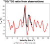 |
Fig. 2 12CO/13CO ratio derived from IRAM Plateau de Bure observations. |
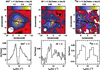 |
Fig. 3 Integrated intensity maps of the HCO+ J = 1 →0, CN N = 1 →0 (J, F = 3/5,5/2 →1/3,3/2), and 13CO J = 1 →0 lines. The velocity range of the integration is from 5 to 15 km s−1. Contour levels are 0.05 to 0.3 in steps of 0.05 Jy beam−1 × km s−1 for HCO+; 0.04 to 0.12 in steps of 0.02 Jy beam−1 × km s−1 for CN; and 0.05 to 0.3 in steps of 0.05 Jy beam−1 × km s−1 for 13CO. The orientation of the molecular emission is approximately perpendicular to the magenta arrow that indicates the direction of the outflow. The black line indicates the disk major axis orientation. The ellipse in the left bottom corner indicates the synthesized beam size. |
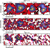 |
Fig. 4 Integrated intensity maps of the HCO+ J = 1 →0, CN N = 1 →0 (J, F = 3/5,5/2 →1/3,3/2), and 13CO J = 1 →0 lines in various velocity intervals. We have avoided the central velocites (9−11 km s−1) for which the space filtering effects are expected important. Contour levels are 0.03 to 0.4 in steps of 0.015 Jy × km s−1 (top panel); 0.02 to 0.12 in steps of 0.02 Jy × km s−1 (middle panel); 0.03 to 0.12 in steps of 0.01 Jy × km s−1 (bottom panel). The orientation of the molecular emission is approximately perpendicular to the magenta arrow that indicates the direction of the outflow. The black line indicates the disk major axis orientation. The ellipse in the left bottom corner indicates the synthesized beam size. |
4 UVES/VLT: critical revision of the spectral type of R Mon
We have estimated the spectral type of R Mon using both stellar SED and UVES emission lines. The first problem when determining the correct spectral type of an embedded B star like R Mon, by fitting the continuum SED, is the treatment of the extinction. As in Alonso-Albi et al. (2009), we used the extinction law of Cardelli et al. (1989). Hernández et al. (2004) discussed the problem of the uncertainties in the extinction law and showed that in embedded Be stars the value of the total to selective absorption, RV, is close to 5, instead of the value of 3.1 commonly assumed for the dust in the galactic plane, due to the prevailing of a population of grains of greater size. The second problem is the possible variability of the source, which means that the observationsshould be obtained the same date. The latest photometry available for R Mon is the data reported by Mendigutía et al. (2012), but the original source of the photometric data used by these authors is Morel & Magnenat (1978), which is the same set of fluxes adopted by Alonso-Albi et al. (2009). Although old data, these UVBRI photometry were taken almost simultaneously so they are not affected by the source variability, showing a B − V color index of 0.61.
Figure 5 shows our fits to the R Mon SED using various values of the spectral type. We use the Kurucz model to predict the stellar photospheric emission. The near-IR excess can be explained by assuming the existence of a disk. At these wavelengths, the dust thermal emission is optically thick and the flux mainly depends on the dust temperature in the disk surface that is determined by the spectral type (Chiang & Goldreich 1997; Dullemond et al. 2001). We show the photospheric emission (green line) and the emission of the circumstellar disk that has been calculated according to the assumed spectral type, using the model described by Alonso-Albi et al. (2009; red line). The UVBRI part of the SED as well as the near-IR excess can only be fitted by assuming RV = 5.0 and a spectral type B0 for R Mon. A spectral type of B8 could only agree with the stellar photometry if we assume RV around 7, but this high value is very difficult to justify.
An independent method to estimate the stellar spectral type is by fitting the UVES emission lines. We plot the fullUVES spectrum of R Mon in relative intensities in the top panel of Fig. 6. The spectrum is full of emission lines, of which the most prominent, from blue to red, are Ca K 3933.66 Å, Hϵ, Hδ, Hγ (P Cygni profiles), Hβ, S II 4925.35, Na I 5889.95, 5895.92 Å (both P Cygni), [O I] 6300.23, 6363.88 Å, Hα, [N II] 6583.45 Å (the nitrogen line at 6548.05 Å is blended with Hα), [S II] 6730.82, 6716.44 Å, and beyond 8500 Å, the Ca II IR triplet (8495.02, 8542.09, 8662.14 Å), and H I Paschen 9–14 (only the completely certain line identifications are listed). In addition, there are many weak and broad features, also in emission, which are the result of blends of many metallic lines. All these emissions are presumably originated by the high accretion rate of this object (see below). The absorptions in the regions beyond 6800, 7400, 8200, and 9000 Å are due to contamination by the Earth’s atmosphere.
The middle and bottom panels of Fig. 6 show the profiles of Hϵ, Hδ, and Hγ. As we pointed out above, the three lines show what seem to be classical P Cygni profiles, which have emission on the red side and absorption on the blue side. The blue wings in absorption of these three lines are virtually the only features for which a comparison with photospheric synthetic spectral models, in order to constrain the spectral type, is feasible.
The programs SYNTHE and ATLAS (Kurucz 1993) fed with the models describing the stratification of the stellar atmospheres (Castelli & Kurucz 2003) have been used for spectral synthesis. Models were computed for four temperatures, namely, 11 000 (spectral type ~B8, plotted in green), 20 000 (red), 25 000 (blue), and 30 000 K (cyan). It is clear that the profile with 11 000 K deviates most from the observations, whereas those in the interval 20 000–30 000 K (spectral type ~B2–B0), although not fittting perfectly, are much closer. Solar abundances and values of log g = 4.0 (typical of a hot star near the MS) and v sini = 50 km s−1 were assumed. Given the total absence of photospheric absorption metallic features, it is impossible to estimate the projected rotational velocity. The value assumed does not have a significant effect on the results. As a test, the relative variation of the widths of Hγ at intensity 0.8 with respect to a continuum at 1.0, between two models with 20 000 K and v sini = 50 and 200 km s−1, is ~ 12%; therefore, the results do not change substantially if a larger rotation rate is used. The synthetic photospheric spectra show absorption features that are not seen in the spectrum of R Mon. This is the case of the prominent features He I 4026.21, 4387.93 Å in the narrow windows shown in Fig. 6. A plausible explanation could be that the high activity of the star manifested as emissions across the whole spectrum erases those lines. Actually, two emissions slightly shifted to the blue appear close to those two wavelengths.
Concerning the accretion in R Mon (Fairlamb et al. 2015; see Sect. 6.1 of that paper) discussed this object and a few other Herbig Be stars. R Mon presents a large blue excess around the Balmer jump when compared with models where accretion is not included. They are unable to give an accretion rate for R Mon within the paradigm of the magnetospheric accretion model: it is not possible to reproduce the large blue excess before the filling factor of accretion shocks on the photosphere saturates, which implies that a different scenario must be invoked for massive Be stars.
Considering the analysis in this section we conclude that R Mon is more likely a B0 star and this is the spectral type that we use hereafter.
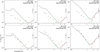 |
Fig. 5 Fit to the UBV RI and JHK photometry assuming different values for the stellar parameters and extinction. The green line indicates the stellar photospheric emission corrected for extinction. The red line is the dust thermal emission coming from the disk. The gray line is the sum of both contributions. |
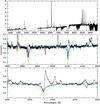 |
Fig. 6 Spectrum of R Mon obtained with the UVES spectrograph on the ESO/VLT. In the middle and bottom panels, synthetic photospheric Kurucz models with temperatures 11 000, 20 000, 25 000, 30 000 K are plotted in green, red, blue, and cyan, respectively. Assuming that the absorption features in the blue side of Hϵ, Hδ, and Hγ have a substantial photospheric contribution, the comparison with the observations suggests that R Mon is an early B-type star with an effective temperature between 20 000 and 30 000 K. |
5 Disk model: 12CO and 13CO lines
Disk modelswith different complexity degrees are used to analyze and interpret line and continuum observations from protoplanetary disks (Jonkheid et al. 2007; Gorti & Hollenbach 2008; Woitke et al. 2009; Kamp et al. 2010; Bruderer et al. 2012; Fedele et al. 2013, 2016). These models are dependent on a wealth of parameters that are usually poorly known and for which one needs to assume a set of reasonable values. The disk mass, flaring, and density structure are key parameters to predict molecular emission. Other parameters such as dust settling, maximum grain size, grain size distribution and grain chemical composition, gas-to-dust mass ratio, and the PAH abundance, also have an impact on the chemistry, energetic balance, and eventually on the predicted line emission (see, e.g., Woitke et al. 2016; Fedele et al. 2016).
The CO lines are expected to be optically thick in most of the disk. Their intensities are hence determined by the gas temperature in the gas layer with τ ~ 1, which is close to the disk surface. Since the different CO rotational lines are excited at different gas kinetic temperatures, the SED of the CO rotational lines is basically tracing the gas temperature profile on the disk surface. For this reason, we decided to adopt a simple power-law model to fit the CO lines. In our approximation, the gas temperature and density are described by the power-law profiles  , Σ ∝ r−p. Even in this simple approximation the number of parameters is too large to be fitted only with the CO observations. Thus, we fixed some of the parameters based on those previously derived from the continuum SED (Alonso-Albi et al. 2009).
The gas mass is fixed to 0.014 M⊙. This value is derived from the disk mass obtained by Alonso-Albi et al. (2009) and adopting a gas-to-dust ratio of 100. An outer radius, Rout = 1500 au, was derived by Fuente et al. (2006) by fitting the size of the compact emission detected in the 12CO 2 →1 line. Since this value is consistent with the size derived for the structure detected in the J, H, and K bands by Murakawa et al. (2008), we kept it in our new fitting. The 12CO abundance is assumed uniform across the disk and equal to 1.6 × 10⁻⁴, which is a reasonable value for a disk in which the gas has temperatures >25–30 K even in the midplane (Alonso-Albi et al. 2010). The adopted stellar parameters are T* = 25 000 K and R* = 4 R⊙, which are those derived from the SED fitting shown in Fig. 5 (RV = 5 and spectral type B0). Since we do not spatially resolve the disk even in the interferometric CO 1 →0 and 2 →1 observations, the values of Tin and Rin cannot be derived independently. In our fitting, we assumed that the gas temperature in the inner edge is equal to the blackbody limit, Tin = (R* /Rin)0.5T*, Rin being a free parameter.
Summarizing, in our procedure, we kept as fixed parameters Md = 0.014 M⊙, X(CO) = 1.6 × 10⁻⁴, and Rout = 1500 au, and varied Rin (from 1 to 100 au, using the corresponding gas temperature Tin), i (from 10° to 50°), p (from 0.5 to 0.7), q (from 1.0 to 2.0) and the turbulent velociy σ (from 0.1 to 5 km s−1) to fit the observations. We used the ray-tracing radiative transfer code DATACUBE2 to model the molecular emission coming from the disk. Using these parameters, we attempted to fit simultaneously our previous interferometric observations of the 12CO 1 →0 and 2 →1 lines published by Fuente et al. (2006) and the PACS data. The interferometric profiles of the 12CO 1 →0 and 2 →1 lines are best fitted assuming Keplerian rotation around a 8 ± 1 M⊙ star and a turbulent dispersion of 0.5 ± 0.3 km s−1. The power-law indexes are fitted to p = 0.60 ± 0.1 and q = 1.8 ± 0.4 (see Table 3). We note that these are the only spectrally resolved line profiles and then the only information about the kinematical disk structure. The value of Rin has a neglible influence on the 12CO 1 →0 and 2 →1 line profiles because of the limited angular resolution and sensitivity of our observations.
In Fig. 7 we compare the PACS fluxes with our model calculations. Thirty-one CO lines with Ju >14 have been observed using PACS. As expected, our model predicts that all these lines are optically thick in the inner disk and only become optically thin at large radii. For a face-on disk, the opacities of the CO J = 14 →13, 19 →18, and 39 →38 lines are lower than 1 for radii larger than ~900, ~400, and ~100 au, respectively. Since ~80% of the emission comes from the optically thick part, different CO abundances and/or small changes of the disk mass only translates into slight differences in the total line fluxes. In addition, the assumed Rout has a negligible impact on the Ju > 30 PACS fluxes as long as Rout > 100 au. Alonso-Albi et al. (2009) obtained an outer radius of 150 ± 50 AU for the dusty disk. Since gaseous disks are usually larger than dusty disks (Facchini et al. 2017), we can reasonably assume thatthe radius of the gaseous disk is larger than this value.
Two different regions are clearly differentiated in the CO SED shown in Fig. 7. Our model falls short of accounting for the fluxes of the mid-J (Ju = 14–30) CO lines. Since the lines are optically thick, increasing the disk gas mass or the CO abundance does not change our results but an increase in the turbulent velocity would certainly translate into an increase in the total line flux. The only way to push up the estimated fluxes to the observed values is to consider a turbulent velocity of ~5 km s−1. However, this value is not consistent with the interferometric CO 1 →0 and 2 →1 profiles. It is also higher than the turbulent velocities observed in other Herbig Ae and T Tauri disks (see, e.g., Piétu et al. 2007). Therefore, we consider that the high Ju = 14−30 CO line fluxes are better explained by some contribution from the envelope and/or outflow to the emission of these lines (Jiménez-Donaire et al. 2017). Taking into account that these lines are unresolved with the PACS spectral and spatial resolution, we favor the interpretation of some contribution from the inner envelope and/or the UV-illuminated walls of the molecular outflow to the Ju = 14–30 lines (Karska et al. 2014). We recall that Alonso-Albi et al. (2009) needed to assume a warm envelope to fit the FIR part of the continuum SED.
In contrast, the fluxes of the Ju > 31 CO lines are slightly overestimated by our model for Rin ≤ 20 au. This suggests the existence of a molecular cavity in the R Mon disk. This result is not unexpected since Alonso-Albi et al. (2009) determined an inner radius of ~18 au for the dusty disk. Furthermore, the continuum SED toward R Mon is better fitted without an inner rim. An optically thick CO disk is not expected in the region depleted in dust (Banzatti et al. 2018). We propose that the disk around the early Be star R Mon is a transition disk by a large inner region depleted in dust and molecular gas, i.e., a low-NIR cavity following the nomenclature of Banzatti et al. (2018). We are aware, however, of the limitations and uncertainties of our model, which are discussed in detail in the next section.
Observational parameters related to the PdBI observations.
Fitting results for the CO emission.
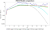 |
Fig. 7 Comparison between PACS observations and our radiative transfer model for different values of the inner CO gap, and assuming a standard 12CO abundance (1.6 × 10⁻⁴). The values for Ju of 1 and 2 are those found by Fuente et al. (2006). |
6 Uncertainties in our model
Our estimate of the inner radius of the gaseous disk is based on the upper limits to the high-J CO lines that are expected to be optically thick for R < 100 au. The total fluxes are then proportional to the gas temperature and the observed line width, which is itself dependent on the disk inclination (because of the Keplerian rotation), gas temperature (thermal dispersion), and turbulent velocity. The key parameter in this result is the value of Tin, which is model dependent. In our simple approximation, we assumed that the gas temperature is the same as the dust temperature in the blackbody limit. For each inner radius, this value depends on the assumed stellar radius and effective temperature. For this reason, it is essential to have an accurate estimate of the the stellar spectral type for our discussion.
But even for a given set of stellar parameters, it is not easy to determine the precise value of the molecular gas temperature in the inner edge of the disk. In principle, it depends on the disk morphology (flaring), grain properties, dust settling, and on the distance from the star. In addition, the cavity could be filled with a tenuous gas and dust that could partially shield the stellar radiation, leading to a lower Tin for the same inner radius. We decided to adopt the blackbody limit to estimate Tin, which is a conservative value. In the illuminated disk surface, the dust is expected to be super-heated to temperatures higher than the blackbody limit (Dullemond et al. 2001). Moreover, the photoelectric effect is an efficient gas heating mechanism in the illuminated surfaces where the gas temperature is expected to be higher than the dust temperature. A more realistic model with detailed thermal balance is expected to produce higher line fluxes and consequently, we get a higher Tin for a given Rin and hence we would need to assume a larger cavity to fit PACS observations.
Although less important, the adopted disk inclination and turbulent velocity also have an impact on the predicted size of the disk cavity. In Fig. 8 we show the total flux of the J = 37 →36 line as a function of inclination and turbulent velocity. The inclination uncertainty has a minor effect because the smaller projected area of the disk at high inclinations is to some extent compensated by the higher velocity gradient along the line of sight. Turbulent velocity is more critical, especially in those regions in which it is comparable to the thermal dispersion. We recall that the value used in our model, ~0.5 km s−1, has been derived from the fitting of theinterferometric 12CO 1 →0 and 2 →1 line profiles. Assuming a lower value of ~0.1 km s−1, similar to that found in low-mass and Herbig Ae stars by Piétu et al. (2007), we would derive an inner radius >10 au to account for the upper limit to the J = 37 →36 line emission.
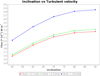 |
Fig. 8 Results of our CO model for line J = 37 →36, calculated for different values of the inclination of the disk and turbulent velocity. |
7 Molecular chemistry: 13CO, CN, HCO+, H2O
We have used a reference model with Rin = 50 au to fit the PdBI observations of 13CO 1 →0 line. We estimate for R Mon a 12C/13C isotopic ratio of 55 ± 15 (Savage et al. 2002). Because of their different optical depths, the emission of the 13CO 1 →0 line is expected to come from a layer closer to the midplane, and thus colder than the layer emitting in 12CO 1 →0. Based on the results of Piétu et al. (2007), we assume that the 13CO 1 →0 line is thermalized and the excitation temperature is half of that corresponding to 12CO, reaching a minimum value around 25 K in the external region of the disk. The resulting spectrum is plotted in left panel of Fig. 9. Because of the low S/N ratio of our 13CO 1 →0 observations and the spatial filtering of the emission in the velocities close to that of the molecular cloud, the two predicted profiles are consistent with our observations.
For CN and HCO+ we used the same model that successfully fit the 12CO and 13CO data to fit the CN and HCO+ observations. In these calculations we assume the same excitation temperature as in the case of the 13CO 1 →0 line and vary the CN and HCO+ abundance to fit the observed spectrum. As a first approximation, we assume that the molecular abundances are uniform along the disk. In Fig. 9, we show the predicted profiles assuming a fractional abundance (wrt H2) of 2 × 10⁻⁸ for CN and 5 × 10⁻⁹ for HCO+. The line profiles predicted by our model are fairly consistent with the observations taking the limitations of our approximation into account.
These abundances are a factor of ~10 larger than the averaged molecular abundances derived in T Tauri and Herbig Ae disks. However, these abundances are similar to those found in photon-dominated regions (see Ginard et al. 2012 and references therein). CN has been widely used as tracer of photon-dominated regions in different environments including reflection nebulae (Fuente et al. 1993, 1995), protoplanetary nebulae (Bachiller & Pérez Gutiérrez 1997), HII regions (Fuente et al. 1996; Rodriguez-Franco et al. 1998; Ginard et al. 2012), and external galaxies (Fuente et al. 2005). While the CN/HCO+ ~1 in dark clouds, a value of ~3 is found in the Orion Bar, very similar to that in the R Mon disk. We are aware that both the absolute value of the abundances and the CN abundance relative to HCO+ are very uncertain because we are using a simple disk model that neglects the density and temperature variations in the vertical direction. Nevertheless, the good agreement between the estimated values and those found in the surface of photon-dominated regions provides further support to the important role played by the stellar UV radiation in the disk evolution.
It is also interesting to comment on the lack of a clear detection of any H2 O line in the PACS spectrum. Within the GASPS project, the water line at ~63 μm has been detected in around 10% of the observed T Tauri (Riviere-Marichalar et al. 2012) and Herbig Ae/Be (Fedele et al. 2012) stars. These lines are interpreted as coming from warm water (Tk > 200 K) in the inner disk region. The nondetection of these high-excitation H2 O lines are also consistent with the presence of a cavity in the circumstellar disk around R Mon.
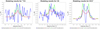 |
Fig. 9 Modeling results for the temperature profile assumed in the 12CO model and for a second profile equal to half of that. 13CO, CN, and HCO+ are shown from left to right panels. |
8 Discussion
Planet formation occurs in protoplanetary disks during the early stages of stellar evolution. These protoplanetary systems evolve from massive disks with a typical gas-to-dust ratio of 100 to optically thin systems similar to our Kuiper Belt. The evolution of the disk is governed by viscous transport (Muzerolle et al. 1998) and photoevaporation (Hollenbach et al. 1994, 2000; Clarke et al. 2001)and models combining both had been successfully used to explain the dispersal of protoplanetary disks around low-mass TTS (Alexander et al. 2006a,b). In the so-called UV-switch model, evolution proceeds mostly through viscous accretion to a point where most accretion stops. From this point on, the gas is quickly dispersed by photoevaporation. This is known as the two timescale problem. Also, planet formation is considered to play a major role in cleaning the inner parts of the disk in the early evolutionof these systems (Zhu et al. 2012). To what extent the same mechanisms can be used to explain the evolution of more massive Herbig Ae/Be stars remains uncertain. Even if mechanisms driving the evolution are the same, we still need to understand the contribution of each of these mechanisms due to the very different mass regimes involved. For instance, photoevaporation is expected to be much more important in Herbig Ae/Be stars than in the low-mass regime.
Alonso-Albi et al. (2009) proposed photoevaporation as the main dispersal mechanism in disks around massive stars. Since the ionizing flux in Herbig Be stars is one order of magnitude higher than in the cooler Herbig Ae and TTS, the timescale for disk photoevaporation is shorter and inner gaps are expected to be formed in a few 0.1 Myr. The characteristic gap radius is the so-called gravitational radius, defined as the radius at which the thermal velocity is equal to the escape velocity and the hot gas overcomes the gravitational field of the star. For a B0 star such as R Mon, the gravitational radius is ~70 au (Alexander et al. 2006b). We used Herschel/PACS spectroscopic observations combined with interferometric observations of the low-J lines of CO and 13CO to derive the size of the inner cavity in the R Mon disk. The upper limits of the Ju > 31 CO lines as measured with PACS are consistent with the existence of an inner cavity with a radius similar to or larger than of that of the dusty disk. The PDR-like chemistry associated with this disk also supports the great influence of the UV radiation in the disk evolution.
9 Summary and conclusions
Our goal is to combine Herschel/PACS data with our interferometric observations at millimeter wavelengths to have a deeper insight into the physics and chemistry of the R Mon disk. Interferometric detections of the HCO+ 1 →0, and CN 1 →0 lines using the IRAM Plateau de Bure Interferometer (PdBI) are presented as well. The HCN 1 →0 line was searched but not detected. In order to constrain the disk model, we re-evaluated the R Mon spectral type using the stellar SED and UVES emission lines. Our analysis confirms that R Mon is a B0 star. Our disk model falls short of predicting the fluxes of the 14 < Ju < 31 lines. Emission coming from the remnant envelope and/or from the UV-illuminated walls of the bipolar outflow could contribute toward increasing the observed value of these lines to some extent. The upper limits of the Ju > 31 CO lines as measured with PACS are consistent with the existence of an inner cavity with a radius similar or larger than that of the dusty disk. The intense emission of the HCO+ and CN lines suggest a strong influence of the UV photons on the gas disk chemistry as well. All the observations gathered thus far are hence consistent with the scenario of R Mon being a transition disk with a cavity of Rin ≳ 20 au. This size is consistent with the photoevaporation radius suggesting that UV photoevaporation could be the main disk dispersal mechanism in massive disks. However, the limited angular resolution of our observations, the absence of velocity resolved profiles of the high-J lines, and the large number of unknown variables in the disk modeling preclude an undoubtful conclusion.
Acknowledgements
We acknowledge the Spanish MINECO for funding support under grants AYA2012-32032. AYA2016-75066-C2-1/2-P and ERC under ERC-2013-SyG, G. A. 610256 NANOCOSMOS. BM is supported by Spanish grant AYA 2014-55840-P. Based on data products from observations made with ESO Telescopes at the Paranal Observatory under program ID 082.C-0831 (PI: Mario Van den Ancker).
Appendix A Additional figures and tables
PACS H2O line fluxes from the central spaxel.
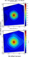 |
Fig. A.1 PACS maps for [OI] lines at 63 and 145 μm. |
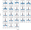 |
Fig. A.2 PACS emission lines and Gaussian fittings for the transitions detected in the central spaxel. |
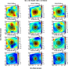 |
Fig. A.3 PACS maps for CO lines in the 74–119 μm range (Jup = 35 to 22). |
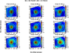 |
Fig. A.4 PACS maps for CO lines in the 124–186 μm range (Jup = 21 to 14). |
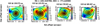 |
Fig. A.5 PACS maps for detected H2O lines. |
References
- Acke, B., van den Ancker, M. E., & Dullemond, C. P. 2005, A&A, 436, 209 [NASA ADS] [CrossRef] [EDP Sciences] [Google Scholar]
- Alexander, R. D., Clarke, C. J., & Pringle, J. E. 2006a, MNRAS, 369, 216 [NASA ADS] [CrossRef] [Google Scholar]
- Alexander, R. D., Clarke, C. J., & Pringle, J. E. 2006b, MNRAS, 369, 229 [NASA ADS] [CrossRef] [Google Scholar]
- Alonso-Albi, T., Fuente, A., Bachiller, R., et al. 2009, A&A, 497, 117 [NASA ADS] [CrossRef] [EDP Sciences] [Google Scholar]
- Alonso-Albi, T., Fuente, A., Crimier, N., et al. 2010, A&A, 518, A52 [NASA ADS] [CrossRef] [EDP Sciences] [Google Scholar]
- Bachiller, R., & Pérez Gutiérrez M. 1997, ApJ, 487, L93 [NASA ADS] [CrossRef] [Google Scholar]
- Banzatti, A., Garufi, A., Kama, M., et al. 2018, A&A, 609, L2 [NASA ADS] [CrossRef] [EDP Sciences] [Google Scholar]
- Boissier, J., Alonso-Albi, T., Fuente, A., et al. 2011, A&A, 531, A50 [NASA ADS] [CrossRef] [EDP Sciences] [Google Scholar]
- Bruderer, S., van Dishoeck, E. F., Doty, S. D., & Herczeg, G. J. 2012, A&A, 541, A91 [NASA ADS] [CrossRef] [EDP Sciences] [Google Scholar]
- Brugel, E. W., Mundt, R., & Buehrke, T. 1984, ApJ, 287, L73 [NASA ADS] [CrossRef] [Google Scholar]
- Canto, J., Rodriguez, L. F., Barral, J. F., & Carral, P. 1981, ApJ, 244, 102 [NASA ADS] [CrossRef] [Google Scholar]
- Cardelli, J. A., Clayton, G. C., & Mathis, J. S. 1989, ApJ, 345, 245 [NASA ADS] [CrossRef] [Google Scholar]
- Castelli, F., & Kurucz, R. L. 2003, Proc. IAU Symp., 210, poster A20 [arXiv:astro-ph/0405087] [Google Scholar]
- Chiang, E. I., & Goldreich, P. 1997, ApJ, 490, 368 [NASA ADS] [CrossRef] [Google Scholar]
- Clarke, C. J., Gendrin, A., & Sotomayor, M. 2001, MNRAS, 328, 485 [NASA ADS] [CrossRef] [Google Scholar]
- Close, L. M., Roddier, F., Hora, J. L., et al. 1997, ApJ, 489, 210 [NASA ADS] [CrossRef] [Google Scholar]
- Cohen, M., Harvey, P. M., & Schwartz, R. D. 1985, ApJ, 296, 633 [NASA ADS] [CrossRef] [Google Scholar]
- Dent, W. R. F., Thi, W. F., Kamp, I., et al. 2013, PASP, 125, 477 [NASA ADS] [CrossRef] [Google Scholar]
- Dullemond, C. P., Dominik, C., & Natta, A. 2001, ApJ, 560, 957 [NASA ADS] [CrossRef] [Google Scholar]
- Dutrey, A., Guilloteau, S., & Guelin, M. 1997, A&A, 317, L55 [NASA ADS] [Google Scholar]
- Facchini, S., Birnstiel, T., Bruderer, S., & van Dishoeck, E. F. 2017, A&A, 605, A16 [NASA ADS] [CrossRef] [EDP Sciences] [Google Scholar]
- Fairlamb, J. R., Oudmaijer, R. D., Mendigutía, I., Ilee, J. D., & van den Ancker, M. E. 2015, MNRAS, 453, 976 [NASA ADS] [CrossRef] [Google Scholar]
- Fedele, D., Bruderer, S., van Dishoeck, E. F., et al. 2012, A&A, 544, L9 [Google Scholar]
- Fedele, D., Bruderer, S., van Dishoeck, E. F., et al. 2013, A&A, 559, A77 [NASA ADS] [CrossRef] [EDP Sciences] [Google Scholar]
- Fedele, D., van Dishoeck, E. F., Kama, M., Bruderer, S., & Hogerheijde, M. R. 2016, A&A, 591, A95 [NASA ADS] [CrossRef] [EDP Sciences] [Google Scholar]
- Fuente, A., Martin-Pintado, J., Cernicharo, J., & Bachiller, R. 1993, A&A, 276, 473 [NASA ADS] [Google Scholar]
- Fuente, A., Martin-Pintado, J., & Gaume, R. 1995, ApJ, 442, L33 [NASA ADS] [CrossRef] [Google Scholar]
- Fuente, A., Rodriguez-Franco, A., & Martin-Pintado, J. 1996, A&A, 312, 599 [NASA ADS] [Google Scholar]
- Fuente, A., Rodríguez-Franco, A., Testi, L., et al. 2003, ApJ, 598, L39 [NASA ADS] [CrossRef] [Google Scholar]
- Fuente, A., García-Burillo, S., Gerin, M., et al. 2005, ApJ, 619, L155 [NASA ADS] [CrossRef] [Google Scholar]
- Fuente, A., Alonso-Albi, T., Bachiller, R., et al. 2006, ApJ, 649, L119 [NASA ADS] [CrossRef] [Google Scholar]
- Ginard, D., González-García, M., Fuente, A., et al. 2012, A&A, 543, A27 [NASA ADS] [CrossRef] [EDP Sciences] [Google Scholar]
- Gorti, U., & Hollenbach, D. 2008, ApJ, 683, 287 [NASA ADS] [CrossRef] [Google Scholar]
- Green, J. D., Evans, II, N. J., Jørgensen, J. K., et al. 2013, ApJ, 770, 123 [NASA ADS] [CrossRef] [Google Scholar]
- Hernández, J., Calvet, N., Briceño, C., Hartmann, L., & Berlind, P. 2004, AJ, 127, 1682 [NASA ADS] [CrossRef] [Google Scholar]
- Hollenbach, D., Johnstone, D., Lizano, S., & Shu, F. 1994, ApJ, 428, 654 [NASA ADS] [CrossRef] [Google Scholar]
- Hollenbach, D. J., Yorke, H. W., & Johnstone, D. 2000, Protostars and Planets IV (Tucson: University of Arizona Press), 401 [Google Scholar]
- Jiménez-Donaire, M. J., Meeus, G., Karska, A., et al. 2017, A&A, 605, A62 [NASA ADS] [CrossRef] [EDP Sciences] [Google Scholar]
- Jones, B. F., & Herbig, G. H. 1982, AJ, 87, 1223 [NASA ADS] [CrossRef] [Google Scholar]
- Jonkheid, B., Dullemond, C. P., Hogerheijde, M. R., & van Dishoeck E. F. 2007, A&A, 463, 203 [NASA ADS] [CrossRef] [EDP Sciences] [Google Scholar]
- Kamp, I., Tilling, I., Woitke, P., Thi, W.-F., & Hogerheijde, M. 2010, A&A, 510, A18 [NASA ADS] [CrossRef] [EDP Sciences] [Google Scholar]
- Karska, A., Herpin, F., Bruderer, S., et al. 2014, A&A, 562, A45 [NASA ADS] [CrossRef] [EDP Sciences] [Google Scholar]
- Kurucz, R. 1993, SYNTHE Spectrum Synthesis Programs and Line Data (Cambridge, MA: Smithsonian Astrophysical Observatory), 18 [Google Scholar]
- Meeus, G., Waters, L. B. F. M., Bouwman, J., et al. 2001, A&A, 365, 476 [NASA ADS] [CrossRef] [EDP Sciences] [Google Scholar]
- Meeus, G., Montesinos, B., Mendigutía, I., et al. 2012, A&A, 544, A78 [NASA ADS] [CrossRef] [EDP Sciences] [Google Scholar]
- Meeus, G., Salyk, C., Bruderer, S., et al. 2013, A&A, 559, A84 [NASA ADS] [CrossRef] [EDP Sciences] [Google Scholar]
- Mendigutía, I., Mora, A., Montesinos, B., et al. 2012, A&A, 543, A59 [NASA ADS] [CrossRef] [EDP Sciences] [Google Scholar]
- Millan-Gabet, R., Schloerb, F. P., & Traub, W. A. 2001, ApJ, 546, 358 [NASA ADS] [CrossRef] [Google Scholar]
- Mora, A., Merin, B., Solano, E., et al. 2001, VizieR Online DataCatalog: J/A+A/378/116 [Google Scholar]
- Morel, M., & Magnenat, P. 1978, A&AS, 34, 477 [NASA ADS] [Google Scholar]
- Murakawa, K., Preibisch, T., Kraus, S., et al. 2008, A&A, 488, L75 [NASA ADS] [CrossRef] [EDP Sciences] [Google Scholar]
- Muzerolle, J., Calvet, N., & Hartmann, L. 1998, ApJ, 492, 743 [NASA ADS] [CrossRef] [Google Scholar]
- Natta, A., Palla, F., Butner, H. M., Evans, II, N. J., & Harvey, P. M. 1993, ApJ, 406, 674 [NASA ADS] [CrossRef] [Google Scholar]
- Pety, J. 2005, in SF2A-2005: Semaine de l’Astrophysique Francaise, eds. F. Casoli, T. Contini, J. M. Hameury, & L. Pagani, 721 [Google Scholar]
- Piétu, V., Dutrey, A., & Guilloteau, S. 2007, A&A, 467, 163 [NASA ADS] [CrossRef] [EDP Sciences] [Google Scholar]
- Podio, L., Kamp, I., Flower, D., et al. 2012, A&A, 545, A44 [NASA ADS] [CrossRef] [EDP Sciences] [Google Scholar]
- Riviere-Marichalar, P., Ménard, F., Thi, W. F., et al. 2012, A&A, 538, L3 [NASA ADS] [CrossRef] [EDP Sciences] [Google Scholar]
- Riviere-Marichalar, P., Merín, B., Kamp, I., Eiroa, C., & Montesinos, B. 2016, A&A, 594, A59 [NASA ADS] [CrossRef] [EDP Sciences] [Google Scholar]
- Rodriguez-Franco, A., Martin-Pintado, J., & Fuente, A. 1998, A&A, 329, 1097 [NASA ADS] [Google Scholar]
- Sandell, G., Weintraub, D. A., & Hamidouche, M. 2011, ApJ, 727, 26 [NASA ADS] [CrossRef] [Google Scholar]
- Savage, C., Apponi, A. J., Ziurys, L. M., & Wyckoff, S. 2002, ApJ, 578, 211 [NASA ADS] [CrossRef] [Google Scholar]
- Sturm, B., Bouwman, J., Henning, T., et al. 2010, A&A, 518, L129 [NASA ADS] [CrossRef] [EDP Sciences] [Google Scholar]
- The, P. S., de Winter, D., & Perez, M. R. 1994, A&AS, 104, 315 [NASA ADS] [Google Scholar]
- van Kempen, T. A., Green, J. D., Evans, N. J., et al. 2010, A&A, 518, L128 [NASA ADS] [CrossRef] [EDP Sciences] [Google Scholar]
- Vink, J. S., Drew, J. E., Harries, T. J., & Oudmaijer, R. D. 2002, MNRAS, 337, 356 [NASA ADS] [CrossRef] [Google Scholar]
- Woitke, P., Kamp, I., & Thi, W.-F. 2009, A&A, 501, 383 [NASA ADS] [CrossRef] [EDP Sciences] [Google Scholar]
- Woitke, P., Min, M., Pinte, C., et al. 2016, A&A, 586, A103 [NASA ADS] [CrossRef] [EDP Sciences] [Google Scholar]
- Zhu, Z., Stone, J. M., & Rafikov, R. R. 2012, ApJ, 758, L42 [NASA ADS] [CrossRef] [Google Scholar]
See http://www.iram.fr/IRAMFR/GILDAS for more information about the GILDAS software (Pety 2005).
This and other modeling tools used by our team can be installed following the instructions provided at conga.oan.es/%7Ealonso/doku.php?id=jparsec.
All Tables
CO line fluxes and widths derived from PACS observations at the central spatial pixel (spaxel).
All Figures
|
Fig. 1 PACS spectroscopic observations from 50 to 190 μm, showing the prominent [OI] emission at 63 μm as well as the CO lines. |
| In the text | |
|
Fig. 2 12CO/13CO ratio derived from IRAM Plateau de Bure observations. |
| In the text | |
|
Fig. 3 Integrated intensity maps of the HCO+ J = 1 →0, CN N = 1 →0 (J, F = 3/5,5/2 →1/3,3/2), and 13CO J = 1 →0 lines. The velocity range of the integration is from 5 to 15 km s−1. Contour levels are 0.05 to 0.3 in steps of 0.05 Jy beam−1 × km s−1 for HCO+; 0.04 to 0.12 in steps of 0.02 Jy beam−1 × km s−1 for CN; and 0.05 to 0.3 in steps of 0.05 Jy beam−1 × km s−1 for 13CO. The orientation of the molecular emission is approximately perpendicular to the magenta arrow that indicates the direction of the outflow. The black line indicates the disk major axis orientation. The ellipse in the left bottom corner indicates the synthesized beam size. |
| In the text | |
|
Fig. 4 Integrated intensity maps of the HCO+ J = 1 →0, CN N = 1 →0 (J, F = 3/5,5/2 →1/3,3/2), and 13CO J = 1 →0 lines in various velocity intervals. We have avoided the central velocites (9−11 km s−1) for which the space filtering effects are expected important. Contour levels are 0.03 to 0.4 in steps of 0.015 Jy × km s−1 (top panel); 0.02 to 0.12 in steps of 0.02 Jy × km s−1 (middle panel); 0.03 to 0.12 in steps of 0.01 Jy × km s−1 (bottom panel). The orientation of the molecular emission is approximately perpendicular to the magenta arrow that indicates the direction of the outflow. The black line indicates the disk major axis orientation. The ellipse in the left bottom corner indicates the synthesized beam size. |
| In the text | |
|
Fig. 5 Fit to the UBV RI and JHK photometry assuming different values for the stellar parameters and extinction. The green line indicates the stellar photospheric emission corrected for extinction. The red line is the dust thermal emission coming from the disk. The gray line is the sum of both contributions. |
| In the text | |
|
Fig. 6 Spectrum of R Mon obtained with the UVES spectrograph on the ESO/VLT. In the middle and bottom panels, synthetic photospheric Kurucz models with temperatures 11 000, 20 000, 25 000, 30 000 K are plotted in green, red, blue, and cyan, respectively. Assuming that the absorption features in the blue side of Hϵ, Hδ, and Hγ have a substantial photospheric contribution, the comparison with the observations suggests that R Mon is an early B-type star with an effective temperature between 20 000 and 30 000 K. |
| In the text | |
|
Fig. 7 Comparison between PACS observations and our radiative transfer model for different values of the inner CO gap, and assuming a standard 12CO abundance (1.6 × 10⁻⁴). The values for Ju of 1 and 2 are those found by Fuente et al. (2006). |
| In the text | |
|
Fig. 8 Results of our CO model for line J = 37 →36, calculated for different values of the inclination of the disk and turbulent velocity. |
| In the text | |
|
Fig. 9 Modeling results for the temperature profile assumed in the 12CO model and for a second profile equal to half of that. 13CO, CN, and HCO+ are shown from left to right panels. |
| In the text | |
|
Fig. A.1 PACS maps for [OI] lines at 63 and 145 μm. |
| In the text | |
|
Fig. A.2 PACS emission lines and Gaussian fittings for the transitions detected in the central spaxel. |
| In the text | |
|
Fig. A.3 PACS maps for CO lines in the 74–119 μm range (Jup = 35 to 22). |
| In the text | |
|
Fig. A.4 PACS maps for CO lines in the 124–186 μm range (Jup = 21 to 14). |
| In the text | |
|
Fig. A.5 PACS maps for detected H2O lines. |
| In the text | |
Current usage metrics show cumulative count of Article Views (full-text article views including HTML views, PDF and ePub downloads, according to the available data) and Abstracts Views on Vision4Press platform.
Data correspond to usage on the plateform after 2015. The current usage metrics is available 48-96 hours after online publication and is updated daily on week days.
Initial download of the metrics may take a while.