| Issue |
A&A
Volume 617, September 2018
|
|
|---|---|---|
| Article Number | A2 | |
| Number of page(s) | 15 | |
| Section | Stellar structure and evolution | |
| DOI | https://doi.org/10.1051/0004-6361/201731628 | |
| Published online | 12 September 2018 | |
Asteroseismic and orbital analysis of the triple star system HD 188753 observed by Kepler
Institut d’Astrophysique Spatiale, CNRS, Université Paris-Sud, Université Paris-Saclay,
Bât. 121,
91405
Orsay Cedex,
France
e-mail: This email address is being protected from spambots. You need JavaScript enabled to view it.
Received:
23
July
2017
Accepted:
8
April
2018
Abstract
Context. The NASA Kepler space telescope has detected solar-like oscillations in several hundreds of single stars, thereby providing a way to determine precise stellar parameters using asteroseismology.
Aims. In this work, we aim to derive the fundamental parameters of a close triple star system, HD 188753, for which asteroseismic and astrometric observations allow independent measurements of stellar masses.
Methods. We used six months of Kepler photometry available for HD 188753 to detect the oscillation envelopes of the two brightest stars. For each star, we extracted the individual mode frequencies by fitting the power spectrum using a maximum likelihood estimation approach. We then derived initial guesses of the stellar masses and ages based on two seismic parameters and on a characteristic frequency ratio, and modelled the two components independently with the stellar evolution code CESTAM. In addition, we derived the masses of the three stars by applying a Bayesian analysis to the position and radial-velocity measurements of the system.
Results. Based on stellar modelling, the mean common age of the system is 10.8 ± 0.2 Gyr and the masses of the two seismic components are MA = 0.99 ± 0.01 M⊙ and MBa = 0.86 ± 0.01 M⊙. From the mass ratio of the close pair, MBb/MBa = 0.767 ± 0.006, the mass of the faintest star is MBb = 0.66 ± 0.01 M⊙ and the total seismic mass of the system is then Msyst = 2.51 ± 0.02 M⊙. This value agrees perfectly with the total mass derived from our orbital analysis, Msyst = 2.51−0.18+0.20 M⊙, and leads to the best current estimate of the parallax for the system, π = 21.9 ± 0.2 mas. In addition, the minimal relative inclination between the inner and outer orbits is 10.9° ± 1.5°, implying that the system does not have a coplanar configuration.
Key words: asteroseismology / binaries: general / stars: evolution / stars: solar-type / astrometry
© ESO 2018
 Open Access article, published by EDP Sciences, under the terms of the Creative Commons Attribution License (http://creativecommons.org/licenses/by/4.0), which permits unrestricted use, distribution, and reproduction in any medium, provided the original work is properly cited.
1 Introduction
Stellar physics has experienced a revolution in recent years with the success of the CoRoT (Baglin et al. 2006) and Kepler space missions (Gilliland et al. 2010a). Thanks to the high-precision photometric data collected by CoRoT and Kepler, asteroseismology has matured into a powerful tool for the characterisation of stars.
The Kepler space telescope yielded unprecedented data allowing the detection of solar-like oscillations in more than 500 stars (Chaplin et al. 2011) and the extraction of mode frequencies for a large number of targets (Appourchaux et al. 2012b; Davies et al. 2016; Lund et al. 2017). From the available sets of mode frequencies, several authors performed detailed modelling to infer the mass, radius, and age of stars (Metcalfe et al. 2014; Silva Aguirre et al. 2015; Creevey et al. 2017). In addition, using scaling relations, the measurement of the seismic parameters Δν and νmax provides a model-free estimate of stellar mass and radius (Chaplin et al. 2011, 2014). A direct measurement of stellar mass and radius can also be obtained using the large frequency separation, Δν, angular diameter from interferometric observations, and parallax (see e.g., Huber et al. 2012; White et al. 2013). The determination of accurate stellar parameters is crucial for studying the populations of stars in our Galaxy (Chaplin et al. 2011; Miglio et al. 2013). Therefore, a proper calibration of the evolutionary models and scaling relations is required in order to derive the stellar mass, radius, and age with a high-level of accuracy. In this context, binary stars provide a unique opportunity to check the consistency of the derived stellar quantities.
Most stars are members of binary or multiple stellar systems. Among all the targets observed by Kepler, there should be many systems showing solar-like oscillations in both components, that is, seismic binaries. However, using population synthesis models, Miglio et al. (2014) predicted that only a small number of seismic binaries are expected to be detectable in the Kepler database. Indeed, the detection of the fainter star requires a magnitude difference between both components typically smaller than approximately one. Until now, only four systems identified as seismic binaries using Kepler photometry have been reported in the literature: 16 Cyg A and B (KIC 12069424 and KIC 12069449; Metcalfe et al. 2012, 2015; Davies et al. 2015), HD 176071 (KIC 9139151 and KIC 9139163; Appourchaux et al. 2012b; Metcalfe et al. 2014), HD 177412 (KIC 7510397; Appourchaux et al. 2015), and HD 176465 (KIC 10124866; White et al. 2017).
The theory of binary star formation excluded the gravitational capture mechanism as an explanation for the existence of binary systems (Tohline 2002). As a consequence, the binary star systems are created from the same dust disk during stellar formation (Tohline 2002). Due to their common origin, both stars of a seismic binary are assumed to have the same age and initial chemical composition, allowing a proper calibration of stellar models. Indeed, the detailed modelling of each star results in two independent values of the stellar age, which can be compared a posteriori. In addition, ground-based observations of a seismic binary also provide strong constraints on the stellar masses through the dynamics of the system. For example, the total mass of the system can be derived from its relative orbit using interferometric measurements. Among the four seismic binaries quoted above, only the pair HD 177412 has a sufficiently short period, namely ~14 yr, to allow the determination of an orbital solution for the system. From the semi-major axis and the period of the relative orbit, Appourchaux et al. (2015) derived the total mass of the system using Kepler’s third law associated with the revised HIPPARCOS parallax of van Leeuwen (2007). However, the parallax of such a binary star can be affected by the orbital motion of the system (Pourbaix 2008), resulting in a potential bias on the estimated values of total mass and stellar radii.
Another approach for measuring stellar masses is to combine spectroscopic and interferometric observations of binary stars. This method has the advantage of allowing a direct determination of distance and individual masses. Such an analysis has recently been performed by Pourbaix & Boffin (2016) for the well-known binary α Cen AB, which showssolar-like oscillations in both components (Bouchy & Carrier 2002; Carrier & Bourban 2003). Thus far, α Cen AB is the only seismic binary for which both a direct comparison between the estimated values of the stellar masses, using asteroseismology and astrometry, and an independent distance measurement are possible. Fortunately, another system offers the possibility of performing such an analysis using Kepler photometry and ground-based observations. This corresponds to a close triple star system, HD 188753, for which we have detected solar-like oscillations in the two brightest components.
This article is organised as follows. Section 2 summarises the main features of HD 188753 and briefly describes the observational data used in this work, including Kepler photometry and ground-based measurements. Section 3 presents the orbital analysis of HD 188753 leading to the determination of the distance and individual masses. Section 4 details the seismic analysis of the two oscillating components, providing accurate mode frequencies and reliable proxies of the stellar masses and ages. Section 5 describes the input physics and optimisation procedure used for the detailed modelling of each of the two stars. Finally, the main results of this paper are presented and discussed in Sect. 6, and some conclusions are drawn in Sect. 7.
2 Target and observations
2.1 Time series and power spectrum
HD 188753 is a bright triple star system (V = 7.41 mag) situated at a distance of 45.7 ± 0.5 pc. The main stellar parameters of the system are given in Table 1. This system was observed by the Kepler space telescope in short-cadence mode (58.85 s sampling; Gilliland et al. 2010b) during a time period of six months, between 2012 March 29 and 2012 October 3. Standard Kepler apertures were not designed for the observation of such a bright and saturated target. A custom aperture was therefore defined and used for HD 188753, through the Kepler Guest Observer (GO) program1, to capture all of the stellar flux.
Short-cadence (SC) photometric data are available to the Kepler Asteroseismic Science Consortium (KASC; Kjeldsen et al. 2010) through the Kepler Asteroseismic Science Operations Center (KASOC) database2. The SC time series for HD 188753 (KIC 6469154) is divided into quarters of three months each, referred to as Q13 and Q14. Custom Aperture File (CAF) observations are handled differently from standard Kepler observations. A specific Kepler catalogue ID3 greater than 100 000 000 is then assigned to each quarter. This work is based on SC data in Data Release 25 (DR25)4, which were processed with the SOC Pipeline 9.3 (Jenkins et al. 2010). As a result, the DR25 SC light curves were corrected for a calibration error affecting the SC pixel data in DR24.
The light curves were concatenated and high-pass filtered using a triangular smoothing with a full width at half maximum (FWHM) ofone day to minimise the effects of long-period instrumental drifts. The single-sided power spectrum was produced using the Lomb-Scargle periodogram (Lomb 1976; Scargle 1982), which has been properly calibrated to comply with Parseval’s theorem (see Appourchaux 2014). The length of data gives a frequency resolution of about 0.06 μHz. Figure 1 shows the smoothed power spectrum of HD 188753 with a zoom-in on the oscillation modes of the secondary seismic component at ~3300 μHz. The significant peak in the PSPS lies at Δν∕2 ≃ 74 μHz, where Δν is the large frequency separation; it corresponds to the signature of the near-regular spacing between individual modes of oscillation for the secondary component. Table 1 provides the seismic parameters of the two stars, Δ ν and νmax, as derived in Sect. 4.2. We note that previous DR24 did not allow the detection of the secondary component in the SC light curves due to the degraded signal-to-noise ratio (S/N).
Main stellar and seismic parameters of HD 188753.
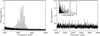 |
Fig. 1 Power spectrum of HD 188753. Left panel: power spectrum smoothed with a 1 μHz boxcar filter showing the oscillation modes of the two seismic components around 2200 and 3300 μHz, respectively. Right panel: zoom-in on the mode power peaks of the secondary component. The inset displays the power spectrum of the power spectrum (PSPS) computed over the frequency range of the oscillations around νmax = 3274 ± 67 μHz (see Table 1). |
2.2 Astrometric and radial-velocity data
HD 188753 (HIP 98001, HO 581, or WDS 19550+4152) is known as a close visual binary discovered by Hough (1899) and characterised by an orbital period of ~25 yr (van Biesbroeck 1918). In the late 1970s, it was established that the secondary component is itself a spectroscopic binary with an orbital period of ~154 days (Griffin 1977). HD 188753 is thus a hierarchical triple star system consisting of a close pair (B) in orbit at a distance of 11.8 AU from the primary component (A).
Position measurements of HD 188753 were first obtained by Hough (1899) with the 18 1 ∕ 2 inch Refractor of the Dearborn Observatory of Northwestern University. This system was then continuously observed over the last century using different techniques and instruments. Since the pioneering work of Struve (1837), more than 150 yr of micrometric measurements are now available for double stars in the literature. Table A.1 provides the result of the micrometric observations for HD 188753. In addition, speckle interferometry for getting the relative position of close binaries has been in use since the 1970’s (Labeyrie et al. 1974). These observations are included in the Fourth Catalog of Interferometric Measurements of Binary Stars (Hartkopf et al. 2001b)5. Table A.2 summarises the high-precision data obtained for HD 188753 from 1979 to 2006. All published data of HD 188753 are displayed in Fig. 2.
The first radial-velocity (RV) observations of HD 188753 were performed by Griffin (1977) from 1969 to 1975 using the photoelectric RV spectrometer of the Cambridge Observatories described in Griffin (1967). The author then discovered that the system contained a spectroscopic binary with an orbital period of ~154 days. HD 188753 was later observed by Konacki (2005) with the high-resolution echelle spectrograph (HIRES; Vogt et al. 1994) at the W. M. Keck Observatory, from 2003 August to 2004 November. Konacki reported the detection of a hot Jupiter around the primary component that was challenged by Eggenberger et al. (2007). However, the author showed that the spectroscopic binary detected by Griffin (1977) corresponds to the secondary component of the visual pair. The system was finally observed by Eggenberger et al. (2007) with the ELODIE echelle spectrograph (Baranne et al. 1996) at the Observatoire de Haute-Provence (France) between July 2005 and August 2006. In order to derive the radial velocities of the faintest star, Mazeh et al. (2009) applied a three-dimensional (3D) correlation technique (TRIMOR) to the data obtained by Eggenberger et al. (2007). In this study, we used the RV measurements from Griffin (1977), Konacki (2005), and Mazeh et al. (2009).
3 Orbital analysis
3.1 Method and model
In this section, we present the methodology employed to determine the orbital parameters of the triple star system HD 188753. For this, we performed a combined treatment of more than a century of archival astrometry (AM) along with the RV measurements found in the literature.
Recently, Appourchaux et al. (2015) derived the orbit of the seismic binary HD 177412 (HIP 93511) by applying a Bayesian analysis to the astrometric measurements of the system. We adapted this Bayesian approach in order to include the radial-velocity measurements for HD 188753. We defined the global likelihood of the data given the orbital parameters as:
 (1)
(1)
where  and
and  are the likelihoods of the AM and RV data respectively, computed from:
 (2)
(2)
 (3)
(3)
NAM and NRV denote the number of available AM and RV observations, respectively, and σ refers to the associated uncertainties. The terms x and y correspond to the coordinates of the orbit on the plane of the sky and denote the declination and right ascension differences, respectively. The term V stands for the radial velocities. The exponents “mod” and “obs” refer to the modelled and observed constraints used during the fitting procedure. Here, the observed positions xobs and yobs are computed from the measured quantities (ρ, θ) by means of the simple relations x = ρcosθ and y = ρsinθ, where ρ is the relative separation and θ is the position angle for both components. Appendix A provides the values of ρ and θ derived from the micrometric and interferometric measurements of HD 188753. In addition, the RV observations Vobs used in this work can be found in Griffin (1977), Konacki (2005), and Mazeh et al. (2009). The theoretical values in Eqs. (2) and (3), namely xmod, ymod, and Vmod, are calculated from the orbital parameters of the system following the observable model described in Appendix B. For the derivation of these orbital parameters, that is,  , we employed a Markov chain Monte Carlo (MCMC) method using the Metropolis-Hastings algorithm (MH; Metropolis et al. 1953; Hastings 1970) as explained in Appendix C.
An essential aspect when combining different data types is the determination of a proper relative weighting. To this end, we performed a preliminary fit of each data set either coming from astrometry or from RV measurements, and calculated the root mean square (rms) of the residuals. Appendix D provides the residual rms derived from the RV measurements of the different authors. In the same way, we derived the residual rms on x and y by fitting the micrometric and interferometric measurements independently. For micrometric measurements, we found σx =25 mas and σy =34 mas while for interferometric measurements, we found σx = 6 mas and σy = 11 mas. We used these values determined after the fitting as weights for the combined fit.
3.2 Orbit of the AB system
We applied the methodology described above in order to derive the best-fit orbital solution of the visual pair, hereafter referred to as the AB system. However, the RV measurements need to be reduced from the 154-day modulation induced by the close pair, hereafter referred to as the Bab sub-system. We then fitted this 154-day modulation as described in Sect. 3.3 (see also Appendix D) to obtain the long-period orbital motion of the AB system.
Figure 2 shows the best-fit solution of the astrometric orbit, plotted with all micrometric and interferometric data listed in Appendix A. The position of the primary component is marked by a plus symbol at the origin of the axes. O−C residuals of the orbital solution are indicated by the solid lines connecting each observation to its predicted position along the orbit. We note that this orbit is listed as grade 1 in the Sixth Catalog of Orbits of Visual Binary Stars (Hartkopf et al. 2001a)6, on a scale of1 (“definitive”) to 5 (“indeterminate”), corresponding to a well-distributed coverage exceeding one revolution. In Fig. 3, we also plotted the radial velocities of the two visual components computed from our best-fit solution. The black line denotes the RV solution of the A component, i.e. the single star, while the grey line denotes the RV solution of the Bab sub-system. For comparison, we added the RV measurements from Griffin (1977), Konacki (2005), and Mazeh et al. (2009), after having removed the 154-day modulation. The final orbital parameters determined from the best-fit solution are given in Table 2.
From these parameters, we can derive the mass of the two components and the semi-major axis of the visual orbit (Heintz 1978):
![Mathematical equation: \begin{eqnarray}M_{A} &=& \frac{1.036 \times 10^{-7} (K_A+K_B)^2\,K_B\,P\,(1-e^2)^{3/2}}{\sin^3 i},\\[5pt] M_{B} &=& \frac{1.036 \times 10^{-7} (K_A+K_B)^2\,K_A\,P\,(1-e^2)^{3/2}}{\sin^3 i},\\[5pt] a _{\textrm{AU}} &=& \frac{9.192 \times 10^{-5} (K_A+K_B)\,P\,(1-e^2)^{1/2}}{\sin i},\end{eqnarray}](/articles/aa/full_html/2018/09/aa31628-17/aa31628-17-eq8.png)
where MA and MB are expressed in units of the solar mass and aAU is expressed in astronomical units. Here, KA and KB are the semi-amplitudes of the radial velocities for both components, in km s−1, P is the orbital period, in days, e is the eccentricity and i is the inclination of the plane of the orbit to the plane of the sky. In addition, the parallax of the system can be determined from the following ratio by combining the AM and RV results:
 (7)
(7)
where πmas is expressed in milliarcseconds. Here, amas denotes the angular semi-major axis derived from the fitting procedure and given in Table 2 while aAU denotes the linear semi-major axis defined in Eq. (6). Table 2 provides the results of the above equations. In order to derive the median and the credible intervals of each physical parameter, namely MA, MB, aAU, and πmas, we calculated Eqs. (4)–(7) using the chains of the orbital parameters.
We found the orbital masses for the single star and the Bab sub-system to be  and
and  , respectively. The total mass of the triple star system is then
  . Additionally, the orbital parallax of the system was found to be π =21.9 ± 0.6 mas. A comparison with the literature results is presented in Sect. 6.2.
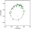 |
Fig. 2 Astrometric orbit of HD 188753. Micrometric observations are indicated by green plus symbols and interferometric observations by blue diamonds. The green lines indicate the distance between the observations and the fitted orbit. A red “H” indicates the HIPPARCOS measure. East is upwards and north is to the right. |
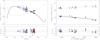 |
Fig. 3 Radial velocities of the two visual components. Left panel: RV measurements of the primary (blue) and secondary (red) components after having removed the 154-day modulation. Squares, circles, and diamonds denote the radial velocities from Griffin (1977), Konacki (2005), and Mazeh et al. (2009), respectively. Right panel: zoom-in on the RV measurements of Mazeh et al. (2009) to show the quality of the fit. The black line denotes the RV solution of the A component while the grey line denotes the RV solution of the B component. |
Orbital and physical parameters of the AB system.
3.3 Orbit of the Bab sub-system
To demonstrate the capacity of their new algorithm, TRIMOR, Mazeh et al. (2009) re-analysed the spectra of HD 188753 obtained by Eggenberger et al. (2007). As a result, they derived the radial velocities of the three stars, allowing them to classify the close pair as a double-lined spectroscopic binary (SB2). We then applied our Bayesian analysis to the RV measurements provided by Mazeh et al. (2009) in their Table 1.
Figure 4 shows the best-fit solution of the radial velocities for both components of the Bab sub-system. We note that in our analysis, we included a linear drift corresponding to the long-period orbital motion of the Bab sub-system. The linear drift and the orbital parameters of the close pair, determined from our best-fit solution, are given in Table D.5. In particular, the Bab sub-system has an eccentricity of 0.175 ± 0.002 and an orbital period of 154.45 ± 0.09 days.
In the case of double-lined spectroscopic binaries, only the quantities MA sin3i and MB sin3i can be derived from Eqs. (4) and (5). These quantities thus provide a lower limit of the stellar masses and a direct estimate of the mass ratio between both stars. From the orbital parameters of the close pair, presented in Table D.5, we obtained MBa sin3iBab = 0.258 ± 0.004 M⊙ and MBb sin3iBab = 0.198 ± 0.002 M⊙. Here, iBab denotes the inclination of the Bab sub-system relative to the plane of the sky. The mass ratio of the close pair is then found to be MBb∕MBa = 0.767 ± 0.006, in agreement with the value of 0.768 ± 0.004 provided by Mazeh et al. (2009). We note that our error estimate of the mass ratio is somewhat larger than that of Mazeh et al. (2009). We suspect that the authors underestimate the uncertainties on their orbital parameters, used in the calculation of the mass ratio, in comparison with our derived values and those of Eggenberger et al. (2007). The advantage of our Bayesian approach is that it yields credible intervals at 16% and 84%, corresponding to the frequentist 1-σ confidence intervals. In the case of HD 188753, the inclination of the close pair can be estimated from its spectroscopic mass sum MB sin3iBab = 0.456 ± 0.006 M⊙. Indeed, the total mass of the Bab sub-system,  , is known from the orbital analysis of the visual pair (see Sect. 3.2). The inclination of the close pair is then found to be iBab = 42.8° ± 1.5°. In addition, wepreviously determined the inclination of the AB system, listed in Table 2, from our combined analysis of the visual orbit. This corresponds to a minimal relative inclination (MRI) between the two orbits of 11.7°± 1.7°. The implicationsof the MRI for such a triple star system will be discussed in Sect. 6.3.
Finally, the inclination iBab can be injected in the quantities MBa sin3iBab = 0.258 ± 0.004 M⊙ and MBb sin3iBab = 0.198 ± 0.002 M⊙ in order to derive the individual masses for both stars of the close pair. We found the orbital masses for stars Ba and Bb to be MBa = 0.83 ± 0.07 M⊙ and 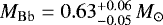 , respectively.In the following, we will compare the orbital masses determined for the three stars of the system with the results of the stellar modelling.
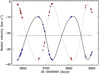 |
Fig. 4 RV measurements of the Ba (blue) and Bb (red) components from Mazeh et al. (2009). The dashed line denotes the long-period orbital motion of the close pair and corresponds to a linear drift towards the positive radial velocities, as can be seen in the right panel of Fig. 3. The black line denotes the RV solution of the Ba component, that is, the most massive star of the close pair, while the grey line denotes the RV solution of the Bb component, the faintest companion. |
4 Seismic data analysis
The goal of this section is to derive accurate mode frequencies and reliable proxies of the stellar masses and ages for the two seismic components of HD 188753. These quantities will then be used for the detailed modelling of each of the two components as explained inSect. 5.2.
4.1 Mode parameter extraction
The extraction of accurate mode frequencies for the two seismic components of HD 188753 is an important step before the stellar modelling. In this work, we adopted a maximum likelihood estimation approach (MLE; Anderson et al. 1990)following the procedure described in Appourchaux et al. (2012b), which has been extensively used during the nominal Kepler mission to provide the mode parameters of a large number of stars (Appourchaux et al. 2012a,b, 2014, 2015).
We repeat here the different steps of this well-suited procedure for completeness:
- 1.
We derive initial guesses of the mode frequencies for the fitting procedure by applying an automated method of detection (see Verner et al. 2011, and references therein) which is based on the values of the seismic parameters, νmax and Δν, that are manually tweaked if required.
- 2.
We fit the power spectrum as the sum of a stellar background made up of a combination of a Lorentzian profile and white noise, as well as a Gaussian oscillation mode envelope with three parameters (the frequency of the maximum mode power, the maximum power, and the width of the mode power).
- 3.
We fit the power spectrum with n orders using the mode profile model described in Appourchaux et al. (2015), with no rotational splitting and the stellar background fixed as determined in step 2.
- 4.
We repeat step 3 but leave the rotational splitting and the stellar inclination angle as free parameters, and then apply a likelihood ratio test to assess the significance of the fitted splitting and inclination angle.
The steps above were used for the main mode power at 2200 μHz, and repeated for the mode power at 3300 μHz. We note that for the secondary component, we used the residual power spectrum derived from the fit of the primary. It corresponds to the ratio between the observed power spectrum and the best fitting model of the primary component, which includes a Lorentzian profile for the stellar background. As a result, the background was modelled with a single white noise component when fitting the mode power at 3300 μHz. The procedure for the quality assurance of the frequencies obtained for both stars is described in Appourchaux et al. (2012b) with a slight modification (for more details, see Appourchaux et al. 2015). The frequencies and their formal uncertainties, derived from the inverse of the Hessian matrix, are provided in Appendix E.
4.2 Stellar parameters from scaling relations
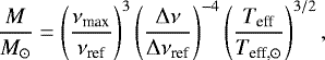
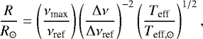
Using the seismic parameters given in Table 1 for stars A and Ba, it is possible to determine their stellar parameters without further advanced modelling. Indeed, the stellar mass and radius of the two seismic components can be estimated from the well-known scaling relations:
 (8)
(8)
 (9)
(9)
where νmax is the frequency of maximum oscillation power, Δν is the large frequency separation, and Teff is the effective temperature of the star. Here, we adopted the reference values from Mosser et al. (2013), νref = 3104 μHz and Δ νref = 138.8 μHz, and the solar effective temperature, Teff,⊙ = 5777 K.
For each seismic component, we derived νmax by fitting a parabola over four (star Ba) or five (star A) monopole modes around the maximum of mode height and Δ ν by fitting the asymptotic relation for frequencies (Tassoul 1980). For star A, we obtained νmax = 2204 ± 8 μHz and Δ ν = 106.96 ± 0.08 μHz, while for star Ba, we obtained νmax = 3274 ± 67 μHz and Δν = 147.42 ± 0.08 μHz. In this work, we adopted the spectroscopic values of the effective temperature from Konacki (2005), Teff,A = 5750 ± 100 K and Teff,Ba = 5500 ± 100 K, measured independently for stars A and Ba. Using Eqs. (8) and (9) with the above values, we then obtained MA = 1.01 ± 0.03 M⊙ and RA = 1.19 ± 0.01 R⊙ for star A, and MBa = 0.86 ± 0.06 M⊙ and RBa = 0.91 ± 0.02 R⊙ for star Ba. The effective temperature of Ba is contaminated by that of Bb. Due to the flux ratio of about 1 to 9 as measured by Mazeh et al. (2009), the temperature of Ba is likely to be 3% lower. With the effective temperature bias due to Bb, the mass and the radius of Ba would be lower by 0.04 M⊙, 0.015 R⊙, respectively; still commensurate with the random errors. We also deduced the luminosity of the two stars from the Stefan–Boltzmann law,  , as LA = 1.40 ± 0.12 L⊙ and LBa = 0.69 ± 0.07 L⊙ (with a bias of −0.1 L⊙ due to the presence of Bb).
Consequently, provided that a measurement of Teff is available, the seismic parameters νmax and Δν give a directestimate of the stellar mass and radius independent of evolutionary models. This so-called direct method has been applied to the hundreds of solar-type stars for which Kepler has detected oscillations (Chaplin et al. 2011, 2014). In the case of HD 188753, the masses derived for each star from the direct method are consistent with the results of our orbital analysis. Therefore, these estimates provide an initial range of mass for stellar modelling.
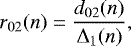
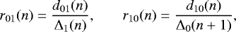
4.3 Frequency separation ratios
In this work, we used the frequency separation ratios as observational constraints for the model fitting, instead of the individual frequencies themselves. Indeed, Roxburgh & Vorontsov (2003) demonstrated that the frequency ratios are approximately independentof the structure of the outer layers and are determined only by the internal structure of the star. They are therefore less sensitive than the individual frequencies to the improper modelling of the near-surface layers (Roxburgh 2005; Otí Floranes et al. 2005) and are also insensitive to the line-of-sight Doppler velocity shifts (Davies et al. 2014). The use of these ratios then allows us to avoid potential biases from applying frequency corrections for near-surfaceeffects (e.g. Kjeldsen et al. 2008; Gruberbauer et al. 2013; Ball & Gizon 2014a,b) and for Doppler shifts.
The frequency separation ratios are defined as:
 (10)
(10)
 (11)
(11)
where d02(n) = νn,0 − νn−1,2 and Δl(n) = νn,l − νn−1,l refer to the small and large separations, respectively. Here, we adopted the five-point smoothed small frequency separations following Roxburgh & Vorontsov (2003):
 (12)
(12)
 (13)
(13)
where ν is the mode frequency, n is the radial order and l is the angular degree. In Fig. 5, we plotted for both stars the ratios r01, r10 and r02 computed from the observed frequencies. A clear oscillatory behaviour of the observed frequency ratios can be seen for star A, in the left panel of Fig. 5, indicating an acoustic glitch. Such a signature arises from the acoustic structure and has already been detected in other solar-like stars (Mazumdar et al. 2014).
Another advantage of using the frequency ratios is that the ratio r02 is sensitive to the structure of the core and hence to the age of the star (Otí Floranes et al. 2005; Lebreton & Montalbán 2009). In particular, White et al. (2011) used the ratio r02 instead of the small frequency separation to construct a modified version of the so-called C-D diagram (Christensen-Dalsgaard 1984), showing that this ratio is an effective indicator of the stellar age. In the case of HD 188753, the mean values of the measured ratios, averaged over the whole range of the observed radial orders, are  and
and  . From these values and those of the large frequency separation listed in Table 1, we can then determine the position of the two seismic components in the modified C-D diagram obtained by White et al. (2011). Using their Fig. 8, we found an age of ~11 Gyr for star A and of ~8.0 Gyr for star Ba.
In addition, Creevey et al. (2017) recently derived a linear relation between the mean value of r02 and the stellar age from the analysis of 57 stars observed by Kepler. Using their Eq. (6) with the above values of ⟨r02 ⟩, we found the individual ages for stars A and Ba to be 9.5 ± 0.2 Gyr and 8.0 ± 0.2 Gyr, respectively. We point out that our estimated errors only result from the propagation of the uncertainties on the measured ratios, since Creevey et al. (2017) do not provide uncertainties on their fitted parameters. The use of the ratio r02 as a proxy of the stellar age therefore allows us to derive an initial range of age for stellar modelling.
5 Stellar modelling
5.1 Input physics
In order to determine precise stellar parameters for HD 188753, we performed a detailed modelling of each seismic component using the stellar evolution code CESTAM (Code d’Évolution Stellaire, avec Transport, Adaptatif et Modulaire; Morel & Lebreton 2008; Marques et al. 2013).
For our model calculations, we adopted the 2005 version of the OPAL equation of state (Rogers & Nayfonov 2002) and the OPAL opacities (Iglesias & Rogers 1996) complemented by those of Alexander & Ferguson (1994) for low temperatures. The opacitytables are given for the new solar mixture derived by Asplund et al. (2009), which corresponds to 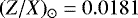 . The microscopic diffusion of helium and heavy elements, including gravitational settling, thermal and concentration diffusion, but no radiative levitation, was taken into account following the prescription of Michaud & Proffitt (1993). We used the NACRE nuclear reaction rates (Angulo et al. 1999) with the revised 14N(p, γ)15O reaction rate from Formicola et al. (2004). Convection was treated according to the mixing-length theory (MLT; Böhm-Vitense 1958) and no overshooting was considered. A standard Eddington gray atmosphere was employed for the atmosphericboundary condition.
5.2 Model optimisation
For each seismic component of HD 188753, we constructed a grid of stellar evolutionary models using CESTAM with the input physics described above. The goodness of fit was evaluated for all of the grid models from the merit function χ2 given by:
 (14)
(14)
where xobs denotes the observational constraints considered, that is, the frequency ratios defined in Eqs. (10) and (11), where xmod denotes the theoretical values predicted by the model and T denotes the transposed matrix. Here, C refers to the covariance matrix of the observational constraints, which is not diagonal due to the strong correlations between the frequency ratios. The theoretical oscillation frequencies used for the calculation of the frequency ratios were computed with the Aarhus adiabatic oscillation package (ADIPLS; Christensen-Dalsgaard 2008).
Firstly, a total of 2000 random grid points were drawn for each star from a reasonable range of the stellar parameters, these being, the age of the star, the mass M, the initial helium abundance Y0, the initial metal-to-hydrogen ratio  and the mixing-length parameter for convection αMLT. Following the age-⟨r02⟩ relation of Creevey et al. (2017), the age of the two stars was assumed to be in the range 5–13 Gyr. For stars A and Ba, we adopted MA ∈ [0.9, 1.2] M⊙ and MBa ∈ [0.7, 1.0] M⊙, respectively, in agreement with the results of the orbital analysis and scaling relations. We considered Y0 ∈ [YP, 0.31] where YP = 0.2477 ± 0.0001 is the primordial value from standard Big Bang nucleosynthesis (Planck Collaboration XVI 2014). The present (Z∕X) ratio can bederived from the observed [Fe/H] value, provided in Table 1, through the relation
 ![Mathematical equation: $[\textrm{Fe}/\textrm{H}] = \log(Z/X) - \log(Z/X) _{\odot}$](/articles/aa/full_html/2018/09/aa31628-17/aa31628-17-eq27.png) . We then estimated the initial
. We then estimated the initial ![Mathematical equation: $[Z/X]_0$](/articles/aa/full_html/2018/09/aa31628-17/aa31628-17-eq28.png) ratio as being in the range 0.01–0.05, which was shifted to a higher value to compensate for diffusion. We adopted αMLT ∈ [1.6, 2] following the solar calibration of Trampedach et al. (2014) that corresponds to αMLT,⊙ = 1.76 ± 0.04.
ratio as being in the range 0.01–0.05, which was shifted to a higher value to compensate for diffusion. We adopted αMLT ∈ [1.6, 2] following the solar calibration of Trampedach et al. (2014) that corresponds to αMLT,⊙ = 1.76 ± 0.04.
Secondly, in order to determine the final parameters of the two stars, we employed a Levenberg–Marquardt minimisation method using the Optimal Stellar Models (OSM)7 software developed by R. Samadi. For star A, we selected the 50 grid models with the lowest χ2 values and used them as a starting point for the final optimisation. We then performed a set of local minimisations adopting the age of the star, the mass, the initial helium abundance, the initial  ratio and the mixing-length parameter as free model parameters. Again, we adopted the merit function defined in Eq. (14) associated with the frequency ratios. For star Ba, due to the limited number of observed ratios, we decided to only adjust the age, the mass, and the initial helium abundance. We then performed a first set of minimisations from the 15 grid models with the lowest χ2 values. During the minimisation process, the initial
  ratio and the mixing-length parameter were fixed at the value of the grid point considered. In order to explore the impact of changing these parameters, we performed a second set of minimisations for the 15 grid models previously selected adopting
 ![Mathematical equation: $(Z/X)_0 = [0.015,0.025,0.035,0.045]$](/articles/aa/full_html/2018/09/aa31628-17/aa31628-17-eq31.png) and αMLT = [1.65, 1.75, 1.85, 1.95] as fixed values. In total, the number of local minimisations for star Ba was 15 + 4 × 4 × 15 = 255. We note that our reference model of star Ba, provided in Table 3, was obtained for
and αMLT = [1.65, 1.75, 1.85, 1.95] as fixed values. In total, the number of local minimisations for star Ba was 15 + 4 × 4 × 15 = 255. We note that our reference model of star Ba, provided in Table 3, was obtained for  and αMLT fixed at their grid-point values.
Figure 5 shows the comparison of the observed frequency ratios (black crosses) with the corresponding values derived from the reference model of each star (red symbols). The modelling results for stars A and Ba are given in Table 3. The error bars on the stellar parameters were derived from the inverse of the Hessian matrix. The normalised χ2 values were computed as  where N denotes the number of observed frequency ratios used for the optimisation.
Reference models for star A and star Ba.
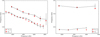 |
Fig. 5 Frequency separation ratios as a function of frequency for star A (left) and star Ba (right). The ratios r01∕10 (n) and r02 (n) derived from the reference model of each star are indicated by red circles and squares, respectively, while the observed ratios are shown as connected points with errors. |
6 Results and discussion
6.1 Physical parameters of HD 188753
From the modelling, we found the individual ages for stars A and Ba to be 10.7 ± 0.2 Gyr and 11.0 ± 0.3 Gyr, respectively. These values are consistent within their error bars, as expected from the common origin of both stars. Combining the individual ages, the system is then about 10.8 ± 0.2 Gyr old.
In addition, the stellar masses from our reference models were found to be MA = 0.99 ± 0.01 M⊙ and MBa = 0.86 ± 0.01 M⊙, which agree very well with the results of the orbital analysis and scaling relations. This latter value can be injected in the mass ratio of the close pair derived in Sect. 3.3, MBb∕MBa = 0.767 ± 0.006, in order to determine the mass of the faintest star with much more precision than in our orbital analysis. The seismic mass of the star Bb is then found to be MBb = 0.66 ± 0.01 M⊙. As a result, the seismic mass of the Bab sub-system is MB = 1.52 ± 0.02 M⊙ and the total seismic mass of the triple star system is Msyst = 2.51 ± 0.02 M⊙. This method provides a precise but model-dependent total mass of the system, which can be compared with the results of our orbital analysis. Indeed, as explained in Sect. 3.2, we obtained a direct estimate of the total mass,  , using the astrometric and RV observations of the system. We find excellent agreement between the seismic and orbital values of the total mass for HD 188753, bolstering our confidence in the results of the stellar modelling.
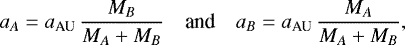
Our stellar models thus provide precise and accurate values of the individual masses that can be used to refine the physical parameters of the system. For example, the semi-major axis of the relative orbit is related to the total mass and to the orbital period of the system from the Kepler’s third law. In other words, the total mass of the system expressed in units of the solar mass is given by 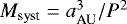 , where aAU is the semi-major axis expressed in astronomical units and P is the orbital period expressed in years. Using the Kepler’s third law with the total seismic mass and the orbital period of the AB system, Msyst = 2.51 ± 0.02 M⊙ and P = 25.63 ± 0.04 yr, we find that the semi-major axis of the relative orbit for the visual pair is aAU = 11.82 ± 0.03 AU. Furthermore, by applying the definition of the centre of mass to the AB system, we can also derive the semi-major axis of the two barycentric orbits with:
 (15)
(15)
where, obviously, aAU = aA + aB. Adopting the seismic masses MA = 0.99 ± 0.01 M⊙ and MB = 1.52 ± 0.02 M⊙ and the above value of the semi-major axis aAU, we then obtain aA = 7.17 ± 0.04 AU and aB = 4.65 ± 0.03 AU. Similarly, the Kepler’s third law and the definition of the centre of mass can be applied to the Bab sub-system using the seismic masses of the close pair. From the above values of MBa and MBb, associated with an orbital period of 154.45 ± 0.09 days, we find that the semi-major axes for star Ba and star Bb are aBa = 0.282 ± 0.002 AU and aBb = 0.367 ± 0.002 AU, respectively.
6.2 Asteroseismic parallax
As explained in Sect. 3.2, the astrometric and RV observations of the visual pair can be combined in order to derive the parallax of the system. The term “orbital parallax” has been suggested to denote a parallax determined in this way (Armstrong et al. 1992). From our combined analysis of the visual pair, we then obtained an orbital parallax of π = 21.9 ± 0.6 mas.
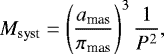
In the case of HD 188753, the precision on the parallax can be improved using the total seismic mass of the system determined in Sect. 6.1. Indeed, combining the Kepler’s third law with Eq. (7) provides a direct relation between the total mass and the parallax of the system:
 (16)
(16)
where Msyst is expressed in units of the solar mass and πmas is expressed in milliarcseconds. Here, amas is the angular semi-major axis of the visual pair, in mas, and P is the orbital period, in years. Adopting the total seismic mass Msyst = 2.51 ± 0.02 M⊙ and the values of amas and P listed in Table 2, we find that the “asteroseismic parallax” of the system is π =21.9 ± 0.2 mas. The error bars on the parallax are estimated through a Monte Carlo simulation using the chains from our Bayesian analysis for amas and P, and a randomised total mass. The probability distributions of the three parameters are then injected in Eq. (16) in order to compute the median and credible intervals for the parallax. We thus obtain a precise estimate of the parallax by combining the asteroseismic and astrometric observations of the system.
As a comparison, the literature values of the parallax for HD 188753 are given in Table 4. Firstly, we note that our results are consistent with the revised HIPPARCOS parallax, π =21.6 ± 0.7 mas, obtained by van Leeuwen (2007). For HD 188753, the author adopted a standard model characterised by five astrometric parameters to describe the apparent motion of the source. These five parameters are the position (α, δ) at the HIPPARCOS epoch, the parallax π and the proper motion (μα*, μδ), and refer to the photocenter of the system. In the case of resolved binaries, it is possible to take the duplicity of the system into account by combining the HIPPARCOS astrometry with existing ground-based observations. For this, Söderhjelm (1999) employed an astrometric model specified by the seven orbital parameters (P, T, e, ω, a, i, Ω), also known as the Campbell elements, in addition to the five parameters quoted above. For HD 188753, Söderhjelm (1999) then obtained a parallax of 21.9 ± 0.6 mas, which is in excellent agreement with the results of our analysis. Using stellar modelling, we thus reduced by a factor of about three the uncertainty on the parallax, which is found independently of the HIPPARCOS data. In addition, the combined treatment of the visual pair, using (visual and speckle) relative positions plus HIPPARCOS data, allows the author to derive the semi-major axis and the orbital period defined in Eq. (16). Knowing the parallax, Söderhjelm (1999) found that the total mass of the system is Msyst = 2.73 ± 0.33 M⊙. The discrepancy between this latter estimate and that reported in this work can be explained by the larger value of the semi-major axis derived by Söderhjelm (1999). However, we point out that our orbital solution results from the derivation of a full orbit using high-resolution techniques, in contrast to that of Söderhjelm (1999).
Unfortunately, there is no available parallax for the system HD 188753 from the Gaia Data Release 1 (DR1; Lindegren et al. 2016). However, as explained in Lindegren et al. (2016), binaries and multiple stellar systems did not receive a special treatment in the data processing. For Gaia DR1, the sources were all treated as single stars. Furthermore, the derived proper motion should be interpreted as the mean motion of the system between the HIPPARCOS epoch (J1991.25) and the Gaia DR1 epoch (J2015.0). The consequence could be that the positions at the two epochs refer to different components of the system, including its photocentre.
Estimated values of the parallax for HD 188753.
6.3 Relative inclination of the two orbits
From our orbital analysis of HD 188753, we derived in Sect. 3.3 an MRI between the visual AB system and the close Bab sub-system of 11.7° ± 1.7°. In particular, we used the orbital value of the mass MB, associated with the quantity MB sin3iBab = 0.456 ± 0.006 M⊙, to estimate the inclination of the Bab sub-system.
As demonstrated in Sect. 6.1, stellar modelling provides precise and accurate values of the individual masses, which can be adopted in our calculations to refine the physical parameters of the system. Using the above value of MB sin3iBab with the seismic mass MB= 1.52 ± 0.02 M⊙, we find that the inclination of the Bab sub-system is iBab = 42.0° ± 0.3°. Since the inclination of the AB system is known (see Table 2), the minimal relative inclination between the two orbits can be precisely determined. We thus obtain a final MRI value of 10.9°± 1.5° for the triple star system HD 188753. Mazeh et al. (2009) attempted to estimate the relative inclination of the system using a similar approach. For this, the authors adopted the total mass of the system provided by Söderhjelm (1999) and the mass ratio of the visual pair from Eggenberger et al. (2007) to determine the mass of the Bab sub-system. The derived value was then injected in Eq. (6) of Mazeh et al. (2009), which is equivalent to the spectroscopic mass sum MB sin3iBab of the close pair. In this way, Mazeh et al. (2009) found that the inclination of the Bab sub-system is iBab = 39.6° ± 2.8° (their Table 3). Considering an inclination for the visual pair of 34° (Söderhjelm 1999)8, the MRI value obtained by Mazeh et al. (2009) from their astrometric approach is about 6°. The advantage of our approach is to provide a more robust estimate of the MRI by combining the modelling results with those derived from the orbital analysis.
The distribution of the relative inclination in triple stars can provide valuable information about the dynamical evolution of multiple stellar systems (Sterzik & Tokovinin 2002). The relative inclination, ϕ, between the two orbital planes is given by (Batten 1973; Fekel 1981):
 (17)
(17)
where i is the orbital inclination, Ω is the position angle of the ascending node and ϕ ∈ [0, π]. Here, the indices “out” and “in” refer to the outer and inner orbits, namely the AB system and the Bab sub-system, respectively. We note that the inclination ϕ also corresponds to the relative angle between the angular momentum vectors of the inner and outer orbits. As a result, the mutual orientation of both orbits is prograde for 0° ≤ ϕ < 90° and retrograde for 90° < ϕ ≤ 180°. In the case of HD 188753, the position angle of the ascending node is totally unknown for the Bab sub-system and thus the relative inclination ϕ cannot be determined. However, it is easy to show from Eq. (17) that iBab − iAB ≤ ϕ ≤ iBab + iAB. From the derived values of iBab and iAB, we then obtain a relative inclination of 10.9° ≤ ϕpro ≤ 73.1° where the lower limit corresponds to the MRI defined above. Since the direction of motion is not known from RV observations, we point out that the orbital inclination of the Bab sub-system may also be iBab = 138.0° ± 0.3°. By symmetry, we then find that 106.9° ≤ ϕretro ≤ 169.1°.
In contrast to the previous analysis of Mazeh et al. (2009), we argue that the triple star system HD 188753 does not have a coplanar configuration. Indeed, we found that the relative inclination between the two orbits may be as high as ~73°, with a lower limit at 10.9° ± 1.5°. For inclined systems, it has been shown that the eccentricity of the inner orbit, ein, and the relative inclination, ϕ, may vary periodically such that the quantity  is conserved. This so-called Lidov-Kozai mechanism (Lidov 1962; Kozai 1962), which takes place when 39.2° ≤ ϕ ≤ 140.8°, plays an important role in the evolution of multiple stellar systems (see e.g. Toonen et al. 2016 for a review). Unfortunately, the suitability of such a mechanism cannot be assessed for our triple star system. However, it is interesting to see how the combined analysis of HD 188753 enabled us to put stringent limits on its relative inclination.
6.4 Impact of the input physics
In this section, we investigate the impact of the input physics on the mass and age of star A. For this, we used the 50 grid models determined in Sect. 5.2 as a starting point for the optimisation. Again, we employed a Levenberg–Marquardt minimisation method to obtain the best-fit model for the different sets of input physics considered.
We remind the reader that our reference model, labelled “Ref” in Table 5, was computed without overshooting, using the solar mixture of Asplund et al. (2009; hereafter AGSS09) and including microscopic diffusion. In order to check the consistency of the derived stellar parameters from our reference model, we then adopted the following input physics during the minimisation process:
Model “Ovsht” computed assuming an overshoot parameter αov = 0.2.
Model “GS98” computed using the solar mixture of Grevesse & Sauval (1998).
Model “Nodiff” computed without microscopic diffusion.
For each case, an optimal model was found by fitting the frequency ratios, as illustrated in Fig. 6. The corresponding stellar parameters are listed in Table 5.
Based on the modelling results, the mass of star A appears to be in the range [0.95, 1.08] M⊙. Unfortunately, the large uncertainty on the orbital value of the mass,  , does not allow us to discard either of the models. In addition, we find the age of star A to be in the range 10.1–11.6 Gyr. As a result, the estimate of the age also suffers from a large uncertainty due to the physics used in the models. On the other hand, the inclusion of overshooting produces a better fit to the frequency ratios (see Fig. 6). For this model, the derived values of the stellar parameters are in good agreement with those from our reference model, thereby reinforcing the results of this study.
We point out that further RV observations of HD 188753 are expected to provide much more stringent constraints on the stellar masses, which should help to disentangle the different input physics. In particular, the choice of the solar mixture requires a dedicated study, which is beyond the scope of this paper.
Derived fundamental parameters of star A for all the models using different input physics.
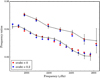 |
Fig. 6 Frequency separation ratios as a function of frequency for star A. Red diamonds correspond to our reference model computed without overshooting while blue diamonds correspond to our optimal model computed with overshooting (αov = 0.2). The observed ratios are shown as connected points with errors. |
7 Conclusions
Using Kepler photometry, we report, for the first time, the detection of solar-like oscillations in the two brightest components of a close triple star system, HD 188753. We performed the seismic analysis of the two stars, providing accurate mode frequencies and reliable proxies of the stellar masses and ages. From the modelling, we also derived precise but model-dependent stellar parameters for the two oscillating components. In particular, we found that the mean common age of the system is 10.8 ± 0.2 Gyr while the masses of the two seismic stars are MA = 0.99 ± 0.01 M⊙ and MBa = 0.86 ± 0.01 M⊙. Furthermore, we explored the impact on the derived stellar parameters of varying the input physics of the models. For star A, the best-fit model was obtained by assuming an overshoot parameter of 0.2.
We also performed the first orbital analysis of HD 188753 that combines both the position and RV measurements of the system. For the wide pair, we derived the masses of the visual components and the parallax of the system, π = 21.9 ± 0.6 mas. In addition, we derived a precise mass ratio between both stars of the close pair, MBb∕MBa = 0.767 ± 0.006. We then found individual masses that are in good agreement with the modelling results. Finally, from the orbital analysis, we estimated the total mass of the system to be 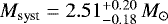 .
.
Combining the asteroseismic and astrometric observations of HD 188753 allowed us to better characterise the main features of this triple star system. For example, using the mass ratio of the close pair, we precisely determined the mass of the faintest star, MBb = 0.66 ± 0.01 M⊙, from the seismic mass of its companion. We then estimated the total seismic mass of the system to be Msyst = 2.51 ± 0.02 M⊙, which agrees perfectly with the orbital value. Injecting this latter into the Kepler’s third law leads to the best current estimate of the parallax for HD 188753, namely π = 21.9 ± 0.2 mas. From our combined analysis, we also derived stringent limits on the relative inclination of the system. With a lower limit at 10.9°± 1.5°, we concluded that HD 188753 does not have a coplanar configuration.
In this work, we demonstrated that binaries and multiple stellar systems have the potential to constrain fundamental stellar parameters, such as the mass and the age. Further observations using asteroseismology and astrometry also promise to improve our knowledge about the dynamical evolution of triple and higher-order systems. In this context, we stress the necessity to prepare catalogues of binaries and multiples for the future space missions TESS (Ricker et al. 2015) and PLATO (Rauer et al. 2014).
Acknowledgements
This paper includes data collected by the Kepler mission. Funding for the Kepler mission is provided by the NASA Science Mission directorate. The authors gratefully acknowledge the Kepler Science Operations Center (SOC) for reprocessingthe short-cadence data that enabled the detection of the secondary seismic component. This research has made use of NASA’s Astrophysics Data System Bibliographic Services, the Washington Double Star Catalog maintained at the US Naval Observatory, the SIMBAD database, operated at CDS, Strasbourg, France and the VizieR catalogue access tool, CDS, Strasbourg, France. The original description of the VizieR service was published in Ochsenbein et al. (2000). Finally, we also thank the anonymous referee for comments that helped to improve this paper.
Appendix A Orbital data
Relative positions of the two visual components from interferometric observations.
Relative positions of the two visual components from interferometric observations.
Appendix B Observable model
The radial velocities VA and VB and the coordinates of the orbit on the plane of the sky (x, y) are calculated from the orbital parameters  by means of the following equations:
![Mathematical equation: \begin{equation*} V_A = V_0 + K_A\,[e\,\,\textrm{cos}\,\omega + \,\textrm{cos}\,(\nu+\omega)], \end{equation*}](/articles/aa/full_html/2018/09/aa31628-17/aa31628-17-eq43.png) (B.1)
(B.1)
![Mathematical equation: \begin{equation*} V_B = V_0 - K_B\,[e\,\,\textrm{cos}\,\omega + \,\textrm{cos}\,(\nu+\omega)], \end{equation*}](/articles/aa/full_html/2018/09/aa31628-17/aa31628-17-eq44.png) (B.2)
(B.2)
 (B.3)
(B.3)
 (B.4)
(B.4)
where V0 is the systemic velocity, KA and KB are the semi-amplitudes of the radial velocities for each component, e is the orbital eccentricity and ω is the argument of periastron. The Thiele-Innes elements A, B, F, and G are given by:
 (B.5)
(B.5)
 (B.6)
(B.6)
 (B.7)
(B.7)
 (B.8)
(B.8)
where a is the semi-major axis of the relative orbit, Ω is the position angle of the line of nodes and i is the inclination of the plane of the orbit to the plane of the sky. The true anomaly ν and the normalized rectangular coordinates in the true orbit (X, Y) are derived as follows:
 (B.9)
(B.9)
 (B.10)
 (B.11)
where E is the eccentric anomaly. This latter can be found using a fixed-point method to solve the Kepler’s equation for any time t:
 (B.12)
where P is the orbital period and T is the time of periastron passage.
Appendix C Bayesianapproach
For derivingthe orbital parameters of HD 188753, we adopted a Bayesian approach as explained below.
According to Bayes’ theorem, the posterior probability of the orbital parameters  given the data D is stated as:
 (C.1)
(C.1)
where  is the prior probability of the orbital parameters, P(D) is the global normalisation likelihood and
  is the likelihood of the
data given the orbital parameters,  , defined in Sect. 3.1. The derivation of the posterior probabilities can be done using the Metropolis–Hastings algorithm (see, as a starting point, Appourchaux 2014). We used a Markov Chain for exploring the space to go from a set
  to another set
  , assuming that either set has the same probability, i.e.
  . The Metropolis–Hastings algorithm requires that we compute the following ratio:
 (C.2)
(C.2)
which is simply the ratio of the likelihood given in Eq. (1). The acceptance probability of the new set,  , is then definedas:
 (C.3)
(C.3)
The new values of the orbital parameters are accepted if β ≤ α, where β is a random number drawn from a uniform distribution over the interval [0, 1], and rejected otherwise.
We set ten chains of 10 million points each with starting points taken randomly from appropriate distributions. The new set of orbital parameters is computed using a random walk as:
 (C.4)
(C.4)
where  is given by a multinomial normal distribution with independent parameters and αrate is an adjustable parameter that is reduced by a factor of two until the rate of acceptance of the new set exceeds 25%. We then derived the posterior probability of each parameter from the chains after rejecting the initial burn-in phase (i.e. the first 10% of each chain). For all parameters, we computed the median and the credible intervals at 16% and 84%, corresponding to a 1-σ interval for a normal distribution. The advantage of this percentile definition over the mode (maximum of the posterior distribution) or the mean (average of the distribution) is that it is conservative with respect to any change of variable over these parameters.
Appendix D Radial-velocity solutions
Orbital solution for star A using the radial-velocity measurements from Griffin (1977).
Orbital solution for star A using the radial-velocity measurements from Konacki (2005).
Orbital solution for star Ba using the radial-velocity measurements from Konacki (2005).
Orbital solution for star A using the radial-velocity measurements from Mazeh et al. (2009).
Orbital solution for stars Ba and Bb using the radial-velocity measurements from Mazeh et al. (2009).
Appendix E Seismic data
Frequencies for star A.
Frequencies for star Ba.
References
- Alexander, D. R., & Ferguson, J. W. 1994, ApJ, 437, 879 [NASA ADS] [CrossRef] [Google Scholar]
- Anderson, E. R., Duvall, Jr. T. L., & Jefferies, S. M. 1990, ApJ, 364, 699 [NASA ADS] [CrossRef] [Google Scholar]
- Angulo, C., Arnould, M., Rayet, M., et al. 1999, Nucl. Phys. A, 656, 3 [NASA ADS] [CrossRef] [Google Scholar]
- Appourchaux, T. 2014, in A Crash Course on Data Analysis in Asteroseismology, eds. P. L. Pallé, & C. Esteban, 123 [Google Scholar]
- Appourchaux, T., Benomar, O., Gruberbauer, M., et al. 2012a, A&A, 537, A134 [NASA ADS] [CrossRef] [EDP Sciences] [Google Scholar]
- Appourchaux, T., Chaplin, W. J., García, R. A., et al. 2012b, A&A, 543, A54 [NASA ADS] [CrossRef] [EDP Sciences] [Google Scholar]
- Appourchaux, T., Antia, H. M., Benomar, O., et al. 2014, A&A, 566, A20 [NASA ADS] [CrossRef] [EDP Sciences] [Google Scholar]
- Appourchaux, T., Antia, H. M., Ball, W., et al. 2015, A&A, 582, A25 [NASA ADS] [CrossRef] [EDP Sciences] [Google Scholar]
- Armstrong, J. T., Mozurkewich, D., Vivekanand, M., et al. 1992, AJ, 104, 241 [NASA ADS] [CrossRef] [Google Scholar]
- Asplund, M., Grevesse, N., Sauval, A. J., & Scott, P. 2009, ARA&A, 47, 481 [NASA ADS] [CrossRef] [Google Scholar]
- Baglin, A., Auvergne, M., Barge, P., et al. 2006, in The CoRoT Mission Pre-Launch Status – Stellar Seismology and Planet Finding, eds. M. Fridlund, A. Baglin, J. Lochard, & L. Conroy, ESA SP, 1306, 33 [Google Scholar]
- Baize, P. 1952, J. Obs., 35, 27 [NASA ADS] [Google Scholar]
- Baize, P. 1954, J. Obs., 37, 73 [NASA ADS] [Google Scholar]
- Baize, P. 1957, J. Obs., 40, 165 [NASA ADS] [Google Scholar]
- Ball, W. H., & Gizon, L. 2014a, A&A, 568, A123 [NASA ADS] [CrossRef] [EDP Sciences] [Google Scholar]
- Ball, W. H., & Gizon, L. 2014b, A&A, 569, C2 [NASA ADS] [CrossRef] [EDP Sciences] [Google Scholar]
- Baranne, A., Queloz, D., Mayor, M., et al. 1996, A&AS, 119, 373 [NASA ADS] [CrossRef] [EDP Sciences] [Google Scholar]
- Batten, A. H. 1973, Binary and Multiple Systems of Stars (Oxford, NY: Pergamon Press), International series of monographs in natural philosophy, 51 [Google Scholar]
- Böhm-Vitense, E. 1958, Z. Astrophys., 46, 108 [Google Scholar]
- Bouchy, F., & Carrier, F. 2002, A&A, 390, 205 [NASA ADS] [CrossRef] [EDP Sciences] [Google Scholar]
- Carrier, F., & Bourban, G. 2003, A&A, 406, L23 [NASA ADS] [CrossRef] [EDP Sciences] [Google Scholar]
- Chaplin, W. J., Kjeldsen, H., Christensen-Dalsgaard, J., et al. 2011, Science, 332, 213 [NASA ADS] [CrossRef] [PubMed] [Google Scholar]
- Chaplin, W. J., Basu, S., Huber, D., et al. 2014, ApJS, 210, 1 [NASA ADS] [CrossRef] [Google Scholar]
- Christensen-Dalsgaard, J. 1984, in Space Research in Stellar Activity and Variability, eds. A. Mangeney, & F. Praderie (Observatoire de Meudon), 11 [Google Scholar]
- Christensen-Dalsgaard, J. 2008, Ap&SS, 316, 113 [NASA ADS] [CrossRef] [Google Scholar]
- Couteau, P. 1967, J. Obs., 50, 41 [NASA ADS] [Google Scholar]
- Couteau, P. 1970, A&AS, 3, 51 [NASA ADS] [Google Scholar]
- Couteau, P., & Ling, J. 1991, A&AS, 88, 497 [NASA ADS] [Google Scholar]
- Couteau, P., Docobo, J. A., & Ling, J. 1993, A&AS, 100, 305 [NASA ADS] [Google Scholar]
- Creevey, O. L., Metcalfe, T. S., Schultheis, M., et al. 2017, A&A, 601, A67 [NASA ADS] [CrossRef] [EDP Sciences] [Google Scholar]
- Davies, G. R., Handberg, R., Miglio, A., et al. 2014, MNRAS, 445, L94 [NASA ADS] [CrossRef] [Google Scholar]
- Davies, G. R., Chaplin, W. J., Farr, W. M., et al. 2015, MNRAS, 446, 2959 [NASA ADS] [CrossRef] [Google Scholar]
- Davies, G. R., Silva Aguirre, V., Bedding, T. R., et al. 2016, MNRAS, 456, 2183 [NASA ADS] [CrossRef] [Google Scholar]
- Eggenberger, A., Udry, S., Mazeh, T., Segal, Y., & Mayor, M. 2007, A&A, 466, 1179 [NASA ADS] [CrossRef] [EDP Sciences] [Google Scholar]
- ESA 1997, The HIPPARCOS and Tycho catalogues, Astrometric and photometric star catalogues derived from the ESA HIPPARCOS Space Astrometry Mission, ESA SP, 1200 [Google Scholar]
- Fekel, Jr. F. C. 1981, ApJ, 246, 879 [NASA ADS] [CrossRef] [Google Scholar]
- Formicola, A., Imbriani, G., Costantini, H., et al. 2004, Phys. Lett. B, 591, 61 [NASA ADS] [CrossRef] [Google Scholar]
- Gilliland, R. L., Brown, T. M., Christensen-Dalsgaard, J., et al. 2010a, PASP, 122, 131 [NASA ADS] [CrossRef] [Google Scholar]
- Gilliland, R. L., Jenkins, J. M., Borucki, W. J., et al. 2010b, ApJ, 713, L160 [NASA ADS] [CrossRef] [Google Scholar]
- Grevesse, N., & Sauval, A. J. 1998, Space Sci. Rev., 85, 161 [Google Scholar]
- Griffin, R. F. 1967, ApJ, 148, 465 [NASA ADS] [CrossRef] [Google Scholar]
- Griffin, R. F. 1977, The Observatory, 97, 15 [NASA ADS] [Google Scholar]
- Gruberbauer, M., Guenther, D. B., MacLeod, K., & Kallinger, T. 2013, MNRAS, 435, 242 [NASA ADS] [CrossRef] [Google Scholar]
- Hartkopf, W. I., & Mason, B. D. 2009, AJ, 138, 813 [NASA ADS] [CrossRef] [Google Scholar]
- Hartkopf, W. I., McAlister, H. A., Mason, B. D., et al. 1997, AJ, 114, 1639 [NASA ADS] [CrossRef] [Google Scholar]
- Hartkopf, W. I., Mason, B. D., McAlister, H. A., et al. 2000, AJ, 119, 3084 [NASA ADS] [CrossRef] [Google Scholar]
- Hartkopf, W. I., Mason, B. D., & Worley, C. E. 2001a, AJ, 122, 3472 [NASA ADS] [CrossRef] [Google Scholar]
- Hartkopf, W. I., McAlister, H. A., & Mason, B. D. 2001b, AJ, 122, 3480 [NASA ADS] [CrossRef] [Google Scholar]
- Hastings, W. K. 1970, Biometrika, 57, 97 [Google Scholar]
- Heintz, W. D. 1975, ApJS, 29, 315 [NASA ADS] [CrossRef] [Google Scholar]
- Heintz, W. D. 1978, Geophysics and Astrophysics Monographs, 15 [Google Scholar]
- Heintz, W. D. 1980, ApJS, 44, 111 [NASA ADS] [CrossRef] [Google Scholar]
- Heintz, W. D. 1990, ApJS, 74, 275 [NASA ADS] [CrossRef] [Google Scholar]
- Heintz, W. D. 1998, ApJS, 117, 587 [NASA ADS] [CrossRef] [Google Scholar]
- Holden, F. 1975, PASP, 87, 253 [NASA ADS] [CrossRef] [Google Scholar]
- Holden, F. 1976, PASP, 88, 325 [NASA ADS] [CrossRef] [Google Scholar]
- Horch, E., Ninkov, Z., van Altena, W. F., et al. 1999, AJ, 117, 548 [NASA ADS] [CrossRef] [Google Scholar]
- Horch, E. P., Robinson, S. E., Meyer, R. D., et al. 2002, AJ, 123, 3442 [NASA ADS] [CrossRef] [Google Scholar]
- Hough, G. W. 1899, Astron. Nachr., 149, 65 [NASA ADS] [CrossRef] [Google Scholar]
- Huber, D., Ireland, M. J., Bedding, T. R., et al. 2012, ApJ, 760, 32 [NASA ADS] [CrossRef] [Google Scholar]
- Huber, D., Silva Aguirre, V., Matthews, J. M., et al. 2014, ApJS, 211, 2 [NASA ADS] [CrossRef] [Google Scholar]
- Iglesias, C. A., & Rogers, F. J. 1996, ApJ, 464, 943 [NASA ADS] [CrossRef] [Google Scholar]
- Jenkins, J. M., Caldwell, D. A., Chandrasekaran, H., et al. 2010, ApJ, 713, L87 [NASA ADS] [CrossRef] [Google Scholar]
- Kjeldsen, H., Bedding, T. R., & Christensen-Dalsgaard, J. 2008, ApJ, 683, L175 [NASA ADS] [CrossRef] [Google Scholar]
- Kjeldsen, H., Christensen-Dalsgaard, J., Handberg, R., et al. 2010, Astron. Nachr., 331, 966 [NASA ADS] [CrossRef] [Google Scholar]
- Konacki, M. 2005, Nature, 436, 230 [NASA ADS] [CrossRef] [PubMed] [Google Scholar]
- Kozai, Y. 1962, AJ, 67, 591 [Google Scholar]
- Labeyrie, A., Bonneau, D., Stachnik, R. V., & Gezari, D. Y. 1974, ApJ, 194, L147 [NASA ADS] [CrossRef] [Google Scholar]
- Lebreton, Y., & Montalbán, J. 2009, in IAU Symp., eds. E. E. Mamajek, D. R. Soderblom, & R. F. G. Wyse, 258, 419 [Google Scholar]
- Lidov, M. L. 1962, Planet. Space Sci., 9, 719 [NASA ADS] [CrossRef] [Google Scholar]
- Lindegren, L., Lammers, U., Bastian, U., et al. 2016, A&A, 595, A4 [NASA ADS] [CrossRef] [EDP Sciences] [Google Scholar]
- Lomb, N. R. 1976, Ap&SS, 39, 447 [Google Scholar]
- Lund, M. N., Silva Aguirre, V., Davies, G. R., et al. 2017, ApJ, 835, 172 [CrossRef] [Google Scholar]
- Marques, J. P., Goupil, M. J., Lebreton, Y., et al. 2013, A&A, 549, A74 [NASA ADS] [CrossRef] [EDP Sciences] [Google Scholar]
- Mason, B. D., Hartkopf, W. I., Wycoff, G. L., et al. 2004, AJ, 128, 3012 [NASA ADS] [CrossRef] [Google Scholar]
- Mason, B. D., Hartkopf, W. I., Raghavan, D., et al. 2011, AJ, 142, 176 [NASA ADS] [CrossRef] [Google Scholar]
- Mazeh, T., Tsodikovich, Y., Segal, Y., et al. 2009, MNRAS, 399, 906 [NASA ADS] [CrossRef] [Google Scholar]
- Mazumdar, A., Monteiro, M. J. P. F. G., Ballot, J., et al. 2014, ApJ, 782, 18 [NASA ADS] [CrossRef] [Google Scholar]
- Metcalfe, T. S., Chaplin, W. J., Appourchaux, T., et al. 2012, ApJ, 748, L10 [NASA ADS] [CrossRef] [Google Scholar]
- Metcalfe, T. S., Creevey, O. L., Doğan, G., et al. 2014, ApJS, 214, 27 [NASA ADS] [CrossRef] [Google Scholar]
- Metcalfe, T. S., Creevey, O. L., & Davies, G. R. 2015, ApJ, 811, L37 [NASA ADS] [CrossRef] [Google Scholar]
- Metropolis, N., Rosenbluth, A. W., Rosenbluth, M. N., Teller, A. H., & Teller, E. 1953, J. Chem. Phys., 21, 1087 [NASA ADS] [CrossRef] [Google Scholar]
- Michaud, G., & Proffitt, C. R. 1993, in IAU Colloq. 137: Inside the Stars, eds. W. W. Weiss, & A. Baglin, ASP Conf. Ser., 40, 246 [Google Scholar]
- Miglio, A., Chiappini, C., Morel, T., et al. 2013, MNRAS, 429, 423 [NASA ADS] [CrossRef] [Google Scholar]
- Miglio, A., Chaplin, W. J., Farmer, R., et al. 2014, ApJ, 784, L3 [NASA ADS] [CrossRef] [Google Scholar]
- Morel, P., & Lebreton, Y. 2008, Ap&SS, 316, 61 [NASA ADS] [CrossRef] [MathSciNet] [Google Scholar]
- Mosser, B., Michel, E., Belkacem, K., et al. 2013, A&A, 550, A126 [NASA ADS] [CrossRef] [EDP Sciences] [Google Scholar]
- Muller, P. 1955, J. Obs., 38, 221 [NASA ADS] [Google Scholar]
- Ochsenbein, F., Bauer, P., & Marcout, J. 2000, A&AS, 143, 23 [NASA ADS] [CrossRef] [EDP Sciences] [Google Scholar]
- Otí Floranes, H., Christensen-Dalsgaard, J., & Thompson, M. J. 2005, MNRAS, 356, 671 [NASA ADS] [CrossRef] [Google Scholar]
- Planck Collaboration XVI. 2014, A&A, 571, A16 [NASA ADS] [CrossRef] [EDP Sciences] [Google Scholar]
- Pourbaix, D. 2008, in A Giant Step: from Milli- to Micro-arcsecond Astrometry, eds. W. J., Jin, I. Platais, & M. A. C. Perryman, IAU Symp., 248,59 [NASA ADS] [Google Scholar]
- Pourbaix, D., & Boffin, H. M. J. 2016, A&A, 586, A90 [NASA ADS] [CrossRef] [EDP Sciences] [Google Scholar]
- Rauer, H., Catala, C., Aerts, C., et al. 2014, Exp. Astron., 38, 249 [NASA ADS] [CrossRef] [Google Scholar]
- Ricker, G. R., Winn, J. N., Vanderspek, R., et al. 2015, J. Astron. Telesc. Instrum. Syst., 1, 014003 [Google Scholar]
- Rogers, F. J., & Nayfonov, A. 2002, ApJ, 576, 1064 [Google Scholar]
- Roxburgh, I. W. 2005, A&A, 434, 665 [NASA ADS] [CrossRef] [EDP Sciences] [Google Scholar]
- Roxburgh, I. W., & Vorontsov, S. V. 2003, A&A, 411, 215 [NASA ADS] [CrossRef] [EDP Sciences] [Google Scholar]
- Scargle, J. D. 1982, ApJ, 263, 835 [Google Scholar]
- Silva Aguirre, V., Davies, G. R., Basu, S., et al. 2015, MNRAS, 452, 2127 [NASA ADS] [CrossRef] [Google Scholar]
- Söderhjelm, S. 1999, A&A, 341, 121 [Google Scholar]
- Sterzik, M. F., & Tokovinin, A. A. 2002, A&A, 384, 1030 [NASA ADS] [CrossRef] [EDP Sciences] [Google Scholar]
- Struve, F. G. W. 1837, Stellarum duplicium et multiplicium mensurae micrometricae per magnum Fraunhoferi tubum annis a 1824 ad 1837 in Specula Dorpatensi institutae (Academiae scientiarum caesareae petropolitanaeifique) [Google Scholar]
- Tassoul, M. 1980, ApJS, 43, 469 [NASA ADS] [CrossRef] [Google Scholar]
- Tohline, J. E. 2002, ARA&A, 40, 349 [NASA ADS] [CrossRef] [Google Scholar]
- Tokovinin, A. A. 1980, Astronomicheskij Tsirkulyar, 1097, 3 [NASA ADS] [Google Scholar]
- Tokovinin, A. A. 1985, A&AS, 61, 483 [NASA ADS] [Google Scholar]
- Toonen, S., Hamers, A., & Portegies Zwart S. 2016, Comput. Astrophys. Cosmol., 3, 6 [CrossRef] [Google Scholar]
- Trampedach, R., Stein, R. F., Christensen-Dalsgaard, J., Nordlund, Å., & Asplund, M. 2014, MNRAS, 445, 4366 [NASA ADS] [CrossRef] [Google Scholar]
- van Biesbroeck G. 1918, AJ, 31, 169 [NASA ADS] [CrossRef] [Google Scholar]
- van Biesbroeck G. 1927, Publications of the Yerkes Observatory, 5, 1 [NASA ADS] [Google Scholar]
- van Biesbroeck G. 1974, ApJS, 28, 413 [NASA ADS] [CrossRef] [Google Scholar]
- van den Bos, W. H. 1959, ApJS, 4, 45 [NASA ADS] [CrossRef] [Google Scholar]
- van den Bos, W. H. 1963, AJ, 68, 57 [NASA ADS] [CrossRef] [Google Scholar]
- van Leeuwen, F. 2007, A&A, 474, 653 [NASA ADS] [CrossRef] [EDP Sciences] [Google Scholar]
- Verner, G. A., Elsworth, Y., Chaplin, W. J., et al. 2011, MNRAS, 415, 3539 [NASA ADS] [CrossRef] [Google Scholar]
- Vogt, S. S., Allen, S. L., Bigelow, B. C., et al. 1994, in Instrumentation in Astronomy VIII, eds. D. L., Crawford, & E. R. Craine, Proc. SPIE, 2198, 362 [Google Scholar]
- White, T. R., Bedding, T. R., Stello, D., et al. 2011, ApJ, 743, 161 [NASA ADS] [CrossRef] [Google Scholar]
- White, T. R., Huber, D., Maestro, V., et al. 2013, MNRAS, 433, 1262 [NASA ADS] [CrossRef] [Google Scholar]
- White, T. R., Benomar, O., Silva Aguirre, V., et al. 2017, A&A, 601, A82 [NASA ADS] [CrossRef] [EDP Sciences] [Google Scholar]
- Worley, C. E. 1962, AJ, 67, 403 [NASA ADS] [CrossRef] [Google Scholar]
Kepler IDs are 100 004 033 and 100 004 071 for Q13 and Q14 respectively.
DR25 corresponds to version 4 of Q13–Q14 for HD 188753.
Söderhjelm (1999) value is not accompanied by error bars.
All Tables
Derived fundamental parameters of star A for all the models using different input physics.
Relative positions of the two visual components from interferometric observations.
Relative positions of the two visual components from interferometric observations.
Orbital solution for star A using the radial-velocity measurements from Griffin (1977).
Orbital solution for star A using the radial-velocity measurements from Konacki (2005).
Orbital solution for star Ba using the radial-velocity measurements from Konacki (2005).
Orbital solution for star A using the radial-velocity measurements from Mazeh et al. (2009).
Orbital solution for stars Ba and Bb using the radial-velocity measurements from Mazeh et al. (2009).
All Figures
|
Fig. 1 Power spectrum of HD 188753. Left panel: power spectrum smoothed with a 1 μHz boxcar filter showing the oscillation modes of the two seismic components around 2200 and 3300 μHz, respectively. Right panel: zoom-in on the mode power peaks of the secondary component. The inset displays the power spectrum of the power spectrum (PSPS) computed over the frequency range of the oscillations around νmax = 3274 ± 67 μHz (see Table 1). |
| In the text | |
|
Fig. 2 Astrometric orbit of HD 188753. Micrometric observations are indicated by green plus symbols and interferometric observations by blue diamonds. The green lines indicate the distance between the observations and the fitted orbit. A red “H” indicates the HIPPARCOS measure. East is upwards and north is to the right. |
| In the text | |
|
Fig. 3 Radial velocities of the two visual components. Left panel: RV measurements of the primary (blue) and secondary (red) components after having removed the 154-day modulation. Squares, circles, and diamonds denote the radial velocities from Griffin (1977), Konacki (2005), and Mazeh et al. (2009), respectively. Right panel: zoom-in on the RV measurements of Mazeh et al. (2009) to show the quality of the fit. The black line denotes the RV solution of the A component while the grey line denotes the RV solution of the B component. |
| In the text | |
|
Fig. 4 RV measurements of the Ba (blue) and Bb (red) components from Mazeh et al. (2009). The dashed line denotes the long-period orbital motion of the close pair and corresponds to a linear drift towards the positive radial velocities, as can be seen in the right panel of Fig. 3. The black line denotes the RV solution of the Ba component, that is, the most massive star of the close pair, while the grey line denotes the RV solution of the Bb component, the faintest companion. |
| In the text | |
|
Fig. 5 Frequency separation ratios as a function of frequency for star A (left) and star Ba (right). The ratios r01∕10 (n) and r02 (n) derived from the reference model of each star are indicated by red circles and squares, respectively, while the observed ratios are shown as connected points with errors. |
| In the text | |
|
Fig. 6 Frequency separation ratios as a function of frequency for star A. Red diamonds correspond to our reference model computed without overshooting while blue diamonds correspond to our optimal model computed with overshooting (αov = 0.2). The observed ratios are shown as connected points with errors. |
| In the text | |
Current usage metrics show cumulative count of Article Views (full-text article views including HTML views, PDF and ePub downloads, according to the available data) and Abstracts Views on Vision4Press platform.
Data correspond to usage on the plateform after 2015. The current usage metrics is available 48-96 hours after online publication and is updated daily on week days.
Initial download of the metrics may take a while.