| Issue |
A&A
Volume 616, August 2018
|
|
|---|---|---|
| Article Number | A133 | |
| Number of page(s) | 7 | |
| Section | The Sun | |
| DOI | https://doi.org/10.1051/0004-6361/201833195 | |
| Published online | 30 August 2018 | |
Temperature gradient in the solar photosphere. Test of a new spectroscopic method and study of its feasibility for ground-based telescopes
1
Université Côte d’Azur, Observatoire de la Côte d’Azur, CNRS UMR 7293 J.L. Lagrange Laboratory, Campus Valrose, 06108 Nice, France
e-mail This email address is being protected from spambots. You need JavaScript enabled to view it.
, This email address is being protected from spambots. You need JavaScript enabled to view it.
2
ISAE-ENSMA-Teleport 2, 1 Avenue Clement Ader, 86360 Chasseneuil-du-Poitou, France
e-mail This email address is being protected from spambots. You need JavaScript enabled to view it.
Received:
9
April
2018
Accepted:
29
May
2018
Abstract
Context. The contribution of quiet-Sun regions to the solar irradiance variability is currently unclear. Some solar-cycle variations of the quiet-Sun physical structure, such as the temperature gradient, might affect the irradiance. The synoptic measurement of this quantity along the activity cycle would improve our understanding of long-term irradiance variations.
Aims. We intend to test a method previously introduced for measuring the photospheric temperature gradient from high-resolution spectroscopic observation and to study its feasibility with ground-based instruments with and without adaptative optics.
Methods. We used synthetic profiles of the FeI 630.15 nm obtained from realistic three-dimensional hydrodynamical simulations of the photospheric granulation and line radiative transfer computations under local thermodynamical equilibrium conditions. Synthetic granulation images at different levels in the line are obtained by convolution with the instrumental point spread function (PSF) under various conditions of atmospheric turbulence, with and without correction by an adaptative optics (AO) system. The PSF are obtained with the PAOLA software, and the AO performances are inspired by the system that will be operating on the Daniel K. Inouye Solar Telescope.
Results. We consider two different conditions of atmospheric turbulence, with Fried parameters of 7 cm and 5 cm, respectively. We show that the degraded images lead to both a bias and a loss of precision in the temperature-gradient measurement, and that the correction with the AO system allows us to drastically improve the measurement quality.
Conclusions. Long-term synoptic observations of the temperature gradient in the solar photosphere can be undertaken by implementing this method on ground-based solar telescopes that are equipped with an AO correction system.
Key words: line: profiles / instrumentation: adaptive optics / techniques: imaging spectroscopy / Sun: fundamental parameters / Sun: photosphere
© ESO 2018
1. Introduction
The variation of the total solar irradiance (TSI) in phase with the solar cycle is now well established thanks to measurements performed in space by dedicated instruments over the past four solar cycles. However, the long-term variations of the TSI at solar minimum are still under debate because different groups that use different composite data find either a constant or a varying TSI at solar minimum. Moreover, the spectral dependance (SSI) of the solar cycle variability is also a controversial subject (see the reviews by Yeo et al. 2014; Solanki et al. 2013). The direct observation of SSI variations on solar-cycle timescales is a difficult task, and some discrepancies appear, in particular in the UV domain, between different space-based instruments. These variations are an important forcing term for the evolution of the climate on Earth. The efforts made to model TSI and SSI variations currently rely on the hypothesis that the main drivers of solar variability are magnetic features at the solar surface, and that the thermodynamical state of the quiet-Sun atmosphere is invariant. Irradiance reconstructions based on the effect of magnetic concentrations at the solar surface allow recovering more than 90% of the observed variations on this timescale. Very recently, Yeo et al. (2017) made a step forward in TSI modeling by using realistic three-dimensional magnetohydrodynamics (MHD) simulations of the solar magnetic concentrations instead of one-dimensional semi-empirical models. The model replicates 95% of the observed variability between April 2010 and July 2016 over the examined timescales (days to years).
Other plausible mechanisms implying a modulation of the global structure of the Sun have also been proposed. Ideas on global structural changes are supported by the observation of the frequencies of the acoustic p-modes that also show a well-documented solar-cycle variation (see Fossat et al. 1987; Salabert et al. 2015). Recent global MHD simulations of the solar convection zone are presented in Cossette et al. (2013). Cyclic large-scale axisymmetric magnetic fields with polarity reversals on decadal timescales are recovered by the simulations, and they show that the thermal convective luminosity varies in phase with the magnetic cycle. However, the simulation domain stops below the photosphere, which limits the type of comparisons that could be made with the real Sun.
Theoretical investigations based on MHD simulations of the properties of the granulation in quiet regions of the Sun in different magnetic environments were presented in Criscuoli (2013). They showed that an ambient magnetic field gives rise to two main physical effects: it inhibits convection, and it reduces the average opacity. The two effects have opposite consequences on the temperature gradients: the reduced opacity, which dominates at optical depths close to unity and smaller, reduces the temperature gradient; but the inhibited convection, which dominates at optical depths larger than one, steepens the temperature gradient. In internetwork regions, the simulations showed that the temperature in the low photosphere decreases with increasing local magnetic field (see also Criscuoli & Uitenbroek 2014). This was later confirmed by Faurobert et al. (2016; hereafter Paper I) where a spectroscopic method for measuring the temperature gradient in the low photosphere was presented and applied to Hinode/SP observations in the FeI 630.15 nm line. The analysis of two sets of observations obtained in December 2007 and December 2013, respectively, showed a decrease in temperature in the low photosphere at the solar maximum in 2013. This finding must be confirmed on a larger set of observations made throughout the solar cycle.
Possible contributions of the quiet Sun to long-term variations of the irradiance could be investigated by a systematic follow-up of the photospheric temperature gradient. As it seems very difficult to ensure constant and controlled instrumental performances over more than one solar cycle on a space-based instrument, synoptic programs dedicated to the measurement of the photospheric temperature gradient should rather be undertaken on ground-based instruments.
Here we present some tests of the measurement method presented in Paper I and a feasibility study for ground-based observations under different conditions of turbulence in the Earth atmosphere, with and without corrections by an AO system. The image degradation at a telescope focus due to atmospheric turbulence is related to the so-called Fried-parameter r0, representing the coherence scale of the turbulent motions. Here we used two values for r0, r0 = 7 cm and r0 = 5 cm. 7 cm is the median value measured at the Haleakala site where the Daniel K. Inouye Solar Telescope (DKIST) is currently under construction, and the case with r0 = 5 cm allows us to investigate more severe turbulence conditions. The point spread functions (PSFs) in the different situations are obtained from the PAOLA sofware (Jolissaint 2006, 2010), and for the characteristics of the adaptative optics (AO), we refer to the description of the system that will operate on DKIST, which was presented in Johnson et al. (2016) and Marino et al. (2016)
In Sect. 2 we explain how the synthetic images of the granulation at different line levels are obtained under different atmospheric turbulence conditions, and we briefly recall the temperature-gradient measurement method (a more detailed presentation is given in Paper I). Section 3 is devoted to the presentation of the results.
2. Measurement method and synthetic images
2.1. Synthetic images
We used a radiative hydrodynamical (RHD) simulation of the Sun taken from the stagger grid (Magic et al. 2013). It was computed using the stagger code, a dedicated (magneto) hydrodynamics code that solves the time-dependent equations for conservation of mass, momentum, and energy. The simulation has 240 × 240 × 240 grid points corresponding to a horizontal extension of 8 Mm and a horizontal resolution of 33.3 km. Then we used the pure local thermal equilibrium (LTE) radiative transfer code OPTIM3D (Chiavassa et al. 2009) to compute synthetic spectra from the snapshots of the RHD simulation. Zero microturbulence was assumed, and the nonthermal Doppler broadening of spectral lines only uses the self-consistent velocity fields directly from the three-dimensional simulations. The temperature and density ranges spanned by the tables are optimized for the values encountered in the RHD simulation. The detailed methods used in the code are explained in Chiavassa et al. (2009). The spectra were computed sampling 115 wavelengths in the interval [630.08 nm, 630.32 nm] with a sampling of 2.1 pm and for different inclinations with respect to the vertical. For a given inclination angle (location on the solar disk), we obtain cubes of simulated (x, y, λ) data that represent solar scenes. We show in Fig. 1 a continuum image obtained at the heliocentric angle θ with cos θ = 0.85 for one snapshot of the RHD simulation.
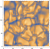 |
Fig. 1. Synthetic image of the granulation in the 630 nm continuum at cos θ = 0.85. The pixel size is 0.045″. |
2.1.1. Without atmospheric turbulence
To obtain synthetic cubes of (x, y, λ) data observed with a telescope, we need to convolve the solar scene with the PSF of the instrument. In a first step, we considered only the image degradation due to the diffraction by the telescope pupil and by the spectrograph slit. For the diffraction, we assumed that the telescope has a 4m diameter off-axis mirror like the DKIST, and the spectrograph profile is a Gaussian function with a half-width of 2.1 pm. Under these very favorable conditions, the spatial resolution (λ/D = 0.0325″) is slightly better than the resolution of the numerical simulation, and the line profiles are only slightly broadened. To compute the convolution of the images with the Airy function, we oversampled the simulated images by a linear interpolation between the grid points. Then we rebinned the images to a pixel size of 0.106″ to account for the width of the spectrograph slit that would be used for this observing program. We also added photon noise and readout noise to the simulated images. To estimate the mean number of photons on each pixel, we assumed an exposure time of 0.5 s, a 4 m telescope, and a pixel size of 0.106″. For the readout noise, we took a value of 20 electrons. Photon noise and readout noise are negligible for such an exposure time. The resulting image in the continuum is shown in Fig. 2.
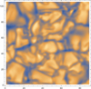 |
Fig. 2. Same image as in Fig. 1 after diffraction by the telescope pupil and rebinning to a pixel size of 0.106″. |
2.1.2. Degraded and AO-corrected images
The previous ideal case is not realistic as turbulence in the Earth atmosphere always degrades the images. To model the PSF of the system (atmosphere + telescope + AO system), we made use of the analytical code PAOLA (Jolissaint 2006, 2010), which adopts a synthetic approach for modeling the performance of an astronomical AO system: the global behavior of the whole system at once is modeled with the help of an analytic expression for the residual phase average (or long-exposure) spatial power spectrum and its relationship with the long-exposure AO optical transfer function. The main advantage of this approach, with respect to a detailed end-to-end Monte Carlo-based approach, is the gain in computation time, which can be particularly enormous in the present case of wide-field correction. We note that an inter-validation study between PAOLA and the well-known end-to-end Monte Carlo-based software tool CAOS (Carbillet et al. 2005) shows a very good agreement for the fundamental fitting error and anisoplanatic error (Carbillet & Jolissain 2012), which are expected to dominate in the present wide-field AO case.
The (relevant) case study of the DKIST and its wide-field AO system being developed has been considered here, and PAOLA was used in its GLAO “full” mode, in which the phase is assumed known in the full sensing field of view defined here by a circle of diameter 10″. Its atmospheric and AO system parameters were taken from Johnson et al. (2016) and Marino et al. (2016), with an expected Fried parameter r0 = 7 cm and a related on-axis Strehl ratio goal of 0.3 at 500 nm. The exact composition of the three-layer median profile taken into account by these authors was kindly communicated to us by Jose Marino. With respect to these assumptions, we have chosen to add a quantity of anisoplanatic error throughout the field of observation, leading to a Strehl ratio of 0.3 as well, but at 630 nm, and we assumed that the resulting PSF is stable throughout the field of observation. In addition, we considered a worse-case scenario with r0 = 5 cm and the same AO system parameters, leading to a Strehl ratio of 0.12 at 630 nm. The parameters of the resulting post-AO PSF modeling are reported in Table 1. These two long-exposure post-AO PSFs, together with the two corresponding seeing-limited PSFs and the ideal PSF (no perturbation at all), are presented in Fig. 3. They were then used for convolution with the various previously modeled solar scenes in order to obtain the final observed images (assuming stability of the correction on the whole field of observation). The resulting images in the continuum are shown in Fig. 4 (r0 = 7 cm) and Fig. 5 (r0 = 5 cm).
Main parameters of the post-AO PSF modeling.
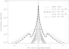 |
Fig. 3. Logarithmic plot of the simulated post-AO and seeing-limited PSFs for the two cases considered (r0 = 7 cm and r0 = 5 cm) and compared with the ideal PSF. |
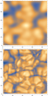 |
Fig. 4. Upper panel: continuum image obtained without AO for atmospheric turbulence r0 = 7 cm for one snapshot of the granulation. Lower panel: continuum image with AO for the same r0 value. The pixel size is 0.106″. |
2.2. From spectrograms to images at constant continuum optical depth
In a spectral line, the opacity varies steeply with the wavelength. It is given by
 (1)
(1)
where kc is the continuum opacity, kl is the frequency-averaged line opacity, λ0 is the line center wavelength in the observer frame, and ϕ is the normalized absorption profile, which in the general case is given by the Voigt function, and ΔλD is the line Doppler width. In the following we use the notations δλ = (λ − λ0)/ΔλD and r = kl/kc. The Doppler broadening is due both to thermal broadening and to unresolved velocities. In the far wings, radiative and collisional damping become dominant.
The absorption profile varies over the solar surface because of temperature, velocity, density, and magnetic inhomogeneities, and the line central wavelength varies as a results of the varying global convective motions of the matter with respect to the observer. The line central wavelength is defined as the position of the minimum of the line-intensity profile.
We first remark that at small line depressions, the shape of the intensity profile is given by I(δλ) ≃ Ic(1 − rϕ(δλ)), where Ic denotes the continuum intensity. It is therefore related to the local values of r and of the line-absorption profile. When we consider for example the image obtained at 2% line depression, it is formed at a constant continuum optical depth surface with rϕ(δλ) = 0:02. The line-cord width at 2% line depression is denoted by Δλc, and its value depends on r and the line absorption profile.
In the damping wings of the line, the profile function decreases like 1/δλ2, so that at δλ = αΔλc, with α < 1, we have rϕ(αΔλc) = (1α2)rϕ(Δλc) = 0.02/α2. The ratio of line to continuous absorption is thus constant over an image at constant α. We may therefore consider that a line-wing image obtained at constant α is formed on a surface where the continuum optical depth is a constant. This approach is valid when r and the line-absorption profile are depth independent or do not vary significantly within the line-wing formation height. For strong lines such as the FeI 630.15 nm line, this would not apply in the line core, which is formed in the upper photosphere. In the following we use this image reconstruction method only in the line-damping wings. To obtain a fine enough depth grid, we chose to define 25 line cords given by δλi = (i − 1)Δλc/24. The damping-wing images are typically at levels 15 to 25, and they are well correlated with the continuum image. Figure 6 shows the images obtained at three different line-levels in the case where the Fried parameter is r0 = 7 cm, and with AO-correction.
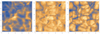 |
Fig. 6. Images at different line levels. The image degradation due to the atmospheric turbulence r0 = 7 cm is corrected by the AO system described in the text. Left panel: line level 1 (line core). Middle panel: line level 8 (granulation-contrast inversion zone). Right panel: line level 15 close to the continuum. |
2.3. Temperature measurement
We wish to measure the mean temperature on constant continuum optical-depth surfaces. Assuming that the FeI 630.15 nm is formed under LTE conditions in the solar photosphere, we may derive the mean temperature from the mean intensity in the images at the different line-levels. The LTE assumption has been tested by various authors (see Shchukina & Trujillo Bueno 2001) who showed that it gives very good results for the average line-profile of the FeI 630 nm line pair on surfaces of several arcseconds2. We also tested the LTE assumption for the average intensity obtained at the different line-levels in the FeI 630.15 nm by comparison with Hinode SOT/SP observations. Figure 7 shows this comparison for observations of the quiet Sun at the solar minimum in 2007. For Hinode data the averages are obtained on 10″ × 10″ surfaces away from network elements. The small differences observed at disk center close to the line center, between the LTE simulations and the observations, might be due to some scattered light in the SOT/SP spectrograph. The agreement is very good at line-levels larger than 10, however, where scattered light (if any) is negligible.
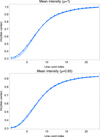 |
Fig. 7. Intensity averaged on a 10″ × 10″ region of the quiet Sun at the 25 line levels normalized to the average continuum intensity at disk center. Dashed line: simulations. Full lines: hinode data. Upper panel: at solar disk-center. Lower panel: at cos ø = 0.85 |
In the following we use synthetic images at line-index larger than 14 at cos ø = 0.85. The mean temperature is derived from the mean intensity in the image using the Planck law. The calibration of the intensity in the simulation to physical units is made using the intensity measured by Neckel (2005) in the solar continuum at 630 nm at cos θ = 0.85: Ic(λ = 630nm, and cos θ = 0.85) = 2.76675 1014 in cgs units.
2.4. Measurement of the formation-depth difference
As in Faurobert et al. (2016), we measured the perspective shift along the radial direction between images taken in a line wing and in the continuum when they are observed away from disk center, that is, at heliocentric angles different from 0.
The image obtained at a line-cord level i, denoted by Ii(x, y), is formed higher in the photosphere than the continuum image Ic(x, y). Because of the perspective effect, Ii(x, y) will appear to be shifted toward the limb in comparison with Ic(x, y) when the images are observed out of disk center. Two-dimensional images are not needed, and one-dimensional spectrograms may be used provided the spectrograph slit is oriented in the radial direction where the perspective shift takes place.
We may therefore consider one-dimensional brightness intensity variations along the slit, which is aligned with the y-axis in the simulations. We therefore obtained spectrograms Ii(x, y) for successive values of x as if we were scanning the solar surface with a slit-spectrograph. This allowed us to record many spectrograms at different x positions to improve the statistics of the solar granulation power spectrum.
Denoting for simplicity with Ii(y) the one-dimensional cuts of the images, we can write
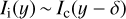 (2)
(2)
and
 (3)
(3)
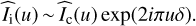
We used a series of spectrograms to estimate the cross-spectrum  between Ic(y) and Ii(y):
 (4)
(4)
where  represents the conjugate Fourier transform of Ii(y), and the brackets refer to the ensemble average.
The perspective displacement introduces a deterministic linear phase-term 2πδu, proportional to the spatial frequency u. The measurement of the phase slope gives the shift and thus the height difference between the surfaces where the images are formed.
We stress here that this method allows us to measure very small displacements between images, as it is not limited by the spatial resolution of the instrument. The main limitation is the signal-to-noise ratio of the granulation spectrum and the domain of validity of Eq. 2, that is, of the assumption of similarity between the line wing and continuum images.
2.5. Continuum formation depth
The method presented above allows us to measure the formation height of line-wing images with respect to the continuum at 630 nm at the same heliocentric angle. To compare the temperature gradient that we measure to standard photospheric models, we need to evaluate the formation height of the 630 nm continuum with respect to the conventional 500 nm continuum formation height that defines the altitude z = 0 in the solar photosphere. To achieve this, we refer to the quiet-Sun model 101 of Fontenla et al. (2011), and we assume that the temperature derived from the mean intensity in the continuum image follows this (T, z) model. This yields the formation height of the 630 nm continuum at the observed heliocentric angle. This means that the continuum point in our (T, z) curves is always, by construction, on the 101 standard model. We stress here again that we can only measure temperature gradients.
3. Results
Figures 8 and 9 show the results of the measurements on three snapshots of the RH simulation, with and without AO, for seeing conditions r0 = 7 cm and 5 cm, respectively. We also show for comparison the standard quiet-Sun model 101 of Fontenla et al. (2011). As we used RH simulations of the granulation with no magnetic field, we expect the temperature gradient to follow the standard quiet-Sun model.
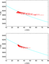 |
Fig. 8. Temperature as a function of altitude for three snapshots of the RH simulation. The bars show one standard deviation on the measurement of the altitude. The blue curve shows the model 101 of Fontenla et al. (2011). Upper panel: measurements from perturbed images with r0 = 7 cm. Lower panel: measurements from images corrected with the AO system. |
Images degraded by atmospheric turbulence lead to both a bias on the temperature gradient and a loss of accuracy (the standard deviation on one measurement increases). When degraded images with r0 = 7 cm are used, the temperature gradient is underestimated, and the typical standard deviation on the altitude is on the order of 15 km. In the worse-case where r0 = 5 cm, the measurement becomes hardly meaningful, with standard deviations on the order of 25 km on the altitude.
However, the image correction by the AO system in both cases allows us to significantly improve the quality and reliability of the measurements. The measured points approach the semi-empirical model very closely, and the standard deviation decreases significantly, to reach values on the order of 5 km. The temperature gradient we measure is then consistent with the standard quiet-Sun model.
4. Conclusion
We have tested a method for measuring the temperature gradient in the low solar photosphere from a ground-based instrument. The method has been applied previously to high-resolution spectroscopic data obtained with the SOT/SP instrument on board the Hinode satellite. It relies on the measurement of the perspective shift between images taken at different levels in a spectral line and in the continuum when observed out of the center of the solar disk. We emphasize that the displacements between structures we seek to measure are not limited by diffraction. A well-known result of astrometry is that it is clearly possible to measure a displacement of an unresolved object far below the resolution of the telescope. In our approach, the displacement is derived from the phase of the cross-spectrum of images at two different line cords. This information may alternatively be derived from the cross-correlation of the images. This technique was first proposed by Beckers & Hege (1982) and later developed for stellar applications (Aime et al. 1984).
Our tests have been performed on simulated images obtained from the STAGGER-code and in the absence of a magnetic field. The FeI 630.15 nm line profile was obtained from a three-dimensional LTE radiative transfer computation. Then the image degradation by the atmospheric turbulence was obtained by convolution with the PSF of the atmosphere + instrument without and with an AO system. The AO system and instrument characteristics were taken from the DKIST performances. We considered two cases of atmospheric turbulence conditions, with Fried parameters r0 = 7 cm and r0 = 5 cm.
We stress that the measurement of the temperature gradient in the solar photosphere from spectroscopic observations is affected by the image degradation due to atmospheric turbulence that induces both a bias and a significant decrease in measurement accuracy. However, the image correction with the AO system allows restoring the quality of the measurement. The temperature gradient we measure on spectrograms derived from the hydrodynamical simulation of the granulation is in agreement with the standard semi-empirical quiet-Sun model of the solar photosphere. This validates the measurement method from high-resolution spectroscopic observations, but corrections with an AO system are mandatory to obtain meaningful results.
References
- Aime, C., Martin, F., Petrov, R., Ricort, G., & Kadiri, S. 1984, A&A, 134, 354 [NASA ADS] [Google Scholar]
- Beckers, J. M., & Hege, E. K. 1982, in Astrophysics and Space Science Library, IAU Colloq. 67: Instrumentation for Astronomy with Large Optical Telescopes, ed. C. M. Humphries, 92, 199 [Google Scholar]
- Carbillet, M., & Jolissain, L. 2012, in 2nd AO4ELT (Adaptive Optics for Extremely Large Telescopes) Conf. [Google Scholar]
- Carbillet, M., Vérinaud, C., Femenía, B., Riccardi, A., & Fini, L. 2005, MNRAS, 356, 1263 [NASA ADS] [CrossRef] [Google Scholar]
- Chiavassa, A., Plez, B., Josselin, E., & Freytag, B. 2009, A&A, 506, 1351 [NASA ADS] [CrossRef] [EDP Sciences] [MathSciNet] [Google Scholar]
- Cossette, J.-F., Charbonneau, P., & Smolarkiewicz, P. K. 2013, ApJ, 777, L29 [NASA ADS] [CrossRef] [Google Scholar]
- Criscuoli, S. 2013, ApJ, 778, 27 [NASA ADS] [CrossRef] [Google Scholar]
- Criscuoli, S., & Uitenbroek, H. 2014, ApJ, 788, 151 [NASA ADS] [CrossRef] [Google Scholar]
- Faurobert, M., Balasubramanian, R., & Ricort, G. 2016, A&A, 595, A71 [NASA ADS] [CrossRef] [EDP Sciences] [Google Scholar]
- Fontenla, J. M., Harder, J., Livingston, W., Snow, M., & Woods, T. 2011, J. Geophys. Res. (Atmos.), 116, 20108 [NASA ADS] [CrossRef] [Google Scholar]
- Fossat, E., Gelly, B., Grec, G., & Pomerantz, M. 1987, A&A, 177, L47 [NASA ADS] [Google Scholar]
- Johnson, L. C., Cummings, K., Drobilek, M., et al. 2016, in Adaptive Optics Systems V, Proc. SPIE, 9909, 99090Y [Google Scholar]
- Jolissaint, L. 2006, PASP, 118, 1205 [NASA ADS] [CrossRef] [Google Scholar]
- Jolissaint, L. 2010, J. Eur. Opt. Soc., 5, 10055 [Google Scholar]
- Magic, Z., Collet, R., Hayek, W., & Asplund, M. 2013, A&A, 560, A8 [NASA ADS] [CrossRef] [EDP Sciences] [Google Scholar]
- Marino, J., Carlisle, E., & Schmidt, D. 2016, in Adaptive Optics Systems V, Proc. SPIE, 9909, 99097C [Google Scholar]
- Neckel, H. 2005, Sol. Phys., 229, 13 [NASA ADS] [CrossRef] [Google Scholar]
- Salabert, D., García, R. A., & Turck-Chièze, S. 2015, A&A, 578, A137 [NASA ADS] [CrossRef] [EDP Sciences] [Google Scholar]
- Shchukina, N., & Trujillo Bueno, J. 2001, ApJ, 550, 970 [NASA ADS] [CrossRef] [Google Scholar]
- Solanki, S. K., Krivova, N. A., & Haigh, J. D. 2013, ARA&A, 51, 311 [NASA ADS] [CrossRef] [Google Scholar]
- Yeo, K. L., Krivova, N. A., & Solanki, S. K. 2014, Space Sci. Rev., 186, 137 [NASA ADS] [CrossRef] [Google Scholar]
- Yeo, K. L., Solanki, S. K., Norris, C. M., et al. 2017, Phys. Rev. Lett., 119, 091102 [NASA ADS] [CrossRef] [Google Scholar]
All Tables
All Figures
|
Fig. 1. Synthetic image of the granulation in the 630 nm continuum at cos θ = 0.85. The pixel size is 0.045″. |
| In the text | |
|
Fig. 2. Same image as in Fig. 1 after diffraction by the telescope pupil and rebinning to a pixel size of 0.106″. |
| In the text | |
|
Fig. 3. Logarithmic plot of the simulated post-AO and seeing-limited PSFs for the two cases considered (r0 = 7 cm and r0 = 5 cm) and compared with the ideal PSF. |
| In the text | |
|
Fig. 4. Upper panel: continuum image obtained without AO for atmospheric turbulence r0 = 7 cm for one snapshot of the granulation. Lower panel: continuum image with AO for the same r0 value. The pixel size is 0.106″. |
| In the text | |
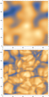 |
Fig. 5. Same as Fig. 4 for r0 = 5 cm. |
| In the text | |
|
Fig. 6. Images at different line levels. The image degradation due to the atmospheric turbulence r0 = 7 cm is corrected by the AO system described in the text. Left panel: line level 1 (line core). Middle panel: line level 8 (granulation-contrast inversion zone). Right panel: line level 15 close to the continuum. |
| In the text | |
|
Fig. 7. Intensity averaged on a 10″ × 10″ region of the quiet Sun at the 25 line levels normalized to the average continuum intensity at disk center. Dashed line: simulations. Full lines: hinode data. Upper panel: at solar disk-center. Lower panel: at cos ø = 0.85 |
| In the text | |
|
Fig. 8. Temperature as a function of altitude for three snapshots of the RH simulation. The bars show one standard deviation on the measurement of the altitude. The blue curve shows the model 101 of Fontenla et al. (2011). Upper panel: measurements from perturbed images with r0 = 7 cm. Lower panel: measurements from images corrected with the AO system. |
| In the text | |
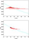 |
Fig. 9. Same as Fig. 8, but with r0 = 5 cm. |
| In the text | |
Current usage metrics show cumulative count of Article Views (full-text article views including HTML views, PDF and ePub downloads, according to the available data) and Abstracts Views on Vision4Press platform.
Data correspond to usage on the plateform after 2015. The current usage metrics is available 48-96 hours after online publication and is updated daily on week days.
Initial download of the metrics may take a while.