| Issue |
A&A
Volume 616, August 2018
|
|
|---|---|---|
| Article Number | A103 | |
| Number of page(s) | 15 | |
| Section | Stellar atmospheres | |
| DOI | https://doi.org/10.1051/0004-6361/201833006 | |
| Published online | 27 August 2018 | |
The shortest-period Wolf-Rayet binary in the Small Magellanic Cloud: Part of a high-order multiple system
Spectral and orbital analysis of SMC AB 6
1
Institut für Physik und Astronomie, Universität Potsdam,
Karl-Liebknecht-Str. 24/25,
14476
Potsdam,
Germany
e-mail: This email address is being protected from spambots. You need JavaScript enabled to view it.
2
Département de physique and Centre de Recherche en Astrophysique du Québec (CRAQ), Université de Montréal,
C.P. 6128, Succ. Centre-Ville,
Montréal,
Québec
H3C 3J7,
Canada
3
Queen’s University 99 University Ave,
Kingston,
Ontario,
Canada
4
American Association of Variable Star Observers,
49 Bay State Road, Cambridge,
MA
02138,
USA
5
Institute of Astrophysics,
KU Leuven, Celestijnenlaan 200 D,
3001
Leuven,
Belgium
Received:
12
March
2018
Accepted:
30
April
2018
Abstract
Context. SMC AB 6 is the shortest-period (P = 6.5 d) Wolf-Rayet (WR) binary in the Small Magellanic Cloud. This binary is therefore a key system in the study of binary interaction and formation of WR stars at low metallicity. The WR component in AB 6 was previously found to be very luminous (log L = 6.3 [L⊙]) compared to its reported orbital mass (≈8 M⊙), placing it significantly above the Eddington limit.
Aims. Through spectroscopy and orbital analysis of newly acquired optical data taken with the Ultraviolet and Visual Echelle Spectrograph (UVES), we aim to understand the peculiar results reported for this system and explore its evolutionary history.
Methods. We measured radial velocities via cross-correlation and performed a spectral analysis using the Potsdam Wolf-Rayet model atmosphere code. The evolution of the system was analyzed using the Binary Population and Spectral Synthesis evolution code.
Results. AB 6 contains at least four stars. The 6.5 d period WR binary comprises the WR primary (WN3:h, star A) and a rather rapidly rotating (veq = 265 km s−1) early O-type companion (O5.5 V, star B). Static N III and N IV emission lines and absorption signatures in He lines suggest the presence of an early-type emission line star (O5.5 I(f), star C). Finally, narrow absorption lines portraying a long-term radial velocity variation show the existence of a fourth star (O7.5 V, star D). Star D appears to form a second 140 d period binary together with a fifth stellar member, which is a B-type dwarf or a black hole. It is not clear that these additional components are bound to the WR binary. We derive a mass ratio of MO∕MWR = 2.2 ± 0.1. The WR star is found to be less luminous than previously thought (log L = 5.9 [L⊙]) and, adopting MO = 41 M⊙ for star B, more massive (MWR = 18 M⊙). Correspondingly, the WR star does not exceed the Eddington limit. We derive the initial masses of Mi,WR = 60 M⊙ and Mi,O = 40 M⊙ and an age of 3.9 Myr for the system. The WR binary likely experienced nonconservative mass transfer in the past supported by the relatively rapid rotation of star B.
Conclusions. Our study shows that AB 6 is a multiple – probably quintuple – system. This finding resolves the previously reported puzzle of the WR primary exceeding the Eddington limit and suggests that the WR star exchanged mass with its companion in the past.
Key words: stars: massive / binaries: spectroscopic / stars: Wolf-Rayet / Magellanic Clouds / stars: individual: SMC AB 6 / stars: atmospheres
© ESO 2018
1 Introduction
The study of massive stars (Mi ≳ 8 M⊙) and binaries at various metallicities is essential for a multitude of astrophysical fields, from supernovae physics to galactic evolution (e.g., Langer 2012). Stars that are massive enough eventually reach the classical Wolf-Rayet (WR) phase that is characterized by powerful stellar winds and hydrogen depletion. Studying WR stars is important both for understanding the evolution of massive stars (e.g., Crowther 2007) and for constraining the energy budget of galaxies (Ramachandran et al. 2018a,b). It is essential to improve our understanding of WR stars especially in the era of gravitational waves.
Two WR-star formation channels have been proposed. First, single massive stars can lose their hydrogen-rich envelopes via powerful radiation-driven winds or eruptions (Conti 1976). Second, mass donors in binary systems, which are expected to be common (e.g., Kiminki & Kobulnicky 2012; Sana et al. 2012; Almeida et al. 2017), may lose their outer layers through mass transfer (Paczynski 1973; Vanbeveren et al. 1998). Since wind mass-loss rates Ṁ scale with metallicity Z (Crowther & Hadfield 2006; Hainich et al. 2015), it is expected that the binary formation channel should become dominant in low metallicity environments (Maeder & Meynet 1994; Bartzakos et al. 2001). The Small Magellanic Cloud (SMC), with ZSMC ≈ 1∕7 Z⊙ (Trundle et al. 2007) and a distance of 62 kpc (Keller & Wood 2006), offers an ideal environment to test this. The reported SMC WR binary fraction is similar to the Galactic WR binary fraction (Foellmi et al. 2003) and the dominance of the binary channel in the SMC is still debated (Shenar et al. 2016; Schootemeijer & Langer 2018).
Our target, SMC AB 6 (AB 6 hereafter), has the shortest period among the five known SMC WR binaries, and hence offers a unique laboratory to investigate the origin of WR stars at low metallicity. Azzopardi & Breysacher (1979) originally classified it as a binary (WN3 + O7 Ia) based on the strong dilution of the WR emission lines and the presence of absorption features in its optical spectrum. Moffat (1982) later proved its binarity based on radial velocity (RV) measurements. The latest orbital study of the system was performed by Foellmi et al. (2003), who classified AB 6 as WN4:+O6.5 I and derived a period of P = 6.5 d. Assuming an inclination of i = 65°, the orbital parameters derived by Foellmi et al. (2003) imply a mass of MWR = 7.5 M⊙, which is comparable with the findings of Hutchings et al. (1984). Despite its relatively low Keplerian mass, the WR primary was reported to have a very high luminosity of log L = 6.3 [L⊙] by Shenar et al. (2016), who analyzed optical and UV spectra of the system. This result placed the WR star significantly above the Eddington limit (Fig. 1). Super-Eddington stars should be unstable on a dynamical timescale, portray strong eruptions, and generally be strongly variable (Shaviv 2001), none of which are observed for AB 6.
These peculiar results encouraged us to acquire high quality UVES spectra of AB 6. The main goal of this study is to explore whether spectra of unprecedented quality can be used to resolve the Eddington limit problem and to investigate the evolutionary history of the shortest-period SMC WR binary. The observations used in this study are described in Sect. 2. In Sect. 3, we illustrate how phase resolved UVES observations reveal the presence of additional components in the spectrum of AB 6. In Sect. 4, we perform an orbital analysis of AB 6, while in Sect. 5 we present a spectral analysis of AB 6. The nature of the system in light of our results is discussed in Sect. 6, and a summary is given in Sect. 7.
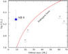 |
Fig. 1 Luminosity and orbital mass originally derived for the WR component of AB 6 by Shenar et al. (2016), compared to the Eddington limit for a fully ionized helium atmosphere. The positions of the other SMC WN stars in binaries are also shown. The values for AB 6 are revised in the present paper. |
2 Observational data
Our study relies predominantly on a spectroscopic dataset obtained with the UVES spectrograph at ESO’s Very Large Telescope in 2017 (ID: 099.D-0766(A), P.I.: Shenar). Altogether 54 individual spectra were obtained with a slit width and a nominal seeing of 1.4′′ during nine nights throughout period 99. The observations were scheduled to allow for an almost evenly spaced coverage of the orbit with Δ ϕ ≈ 0.1. During each night, six exposures covering the blue (3730−5000 Å) and red (5655−9464Å) spectral bands were secured. The spectra were co-added for each of the nine distinct phases and were calibrated to a heliocentric frame of reference. A log of the co-added spectra can be found in Table 1. Since we do not require an extremely precise wavelength calibration, we relied on the default data reduction provided by the ESO archive. The standard setting DIC-2 437+760 was used. With a total exposure time of 50 min per night, a signal-to-noise ratio (S/N) of ≈ 100−130 in the blue band and ≈ 80−100 in the red band at a resolving power of R ≈ 30 000 was obtained. Phases given below correspond to the ephemeris in Table 2.
Several UV spectra were retrieved from the Mikulski Archive for Space Telescopes (MAST). A flux-calibrated, large-aperture IUE spectrum (swp15908, PI: Burki, ϕ = 0.18), covering the range 1150−1980 Å with R ≈ 10 000 and S∕N ≈ 25, was used for detailed spectroscopy and fitting of the total spectral energy distribution (SED). A low dispersion IUE spectrum (lwr04256, PI: Savage, ϕ = 0.18) covering 1850−3350 Å with R ≈ 150 and S∕N ≈ 0 was used for fitting the SED alone. We used high dispersion Hubble Space Telescope (HST) spectra taken with the High Resolution Spectrograph (HRS) and the G160M grating (Z0NG0402T, Z0Z30202T, Z0Z30402T, Z0Z30602T, PI: Hutchings) that cover primarily the C IV λλ1548, 1551 doublet (1528−1563 Å, R ≈ 15 000, S∕N ≈ 30), corresponding to the phases ϕ = 0.99, 0.03, 0.98, and 0.49, respectively. Finally, a FUSE spectrum covering 900−1190 Å with R ≈ 15 000 and S∕N ≈ 25 was also used for detailed spectroscopy and SED fitting (p1030401000, PI: Sembach, ϕ =0.06). We checked for possible source contamination of the IUE and FUSE spectra. The IUE large aperture does not cover any sources that can significantly contribute to the UV flux. The FUSE spectrum could, in principle, be contaminated by nearby sources, depending on the positioning. However, the flux levels of the HST, IUE, and FUSE spectra are consistent within 5%, implying that they are not contaminated by other sources.
UBV band photometry was obtained from Mermilliod (2006). Near-infrared photometry (J, H, KS) was obtained from Cutri et al. (2003), while WISE photometry is available from Cutri & et al. (2012). Finally, IRAC photometry was taken from a compilation by Bonanos et al. (2010).
Log of UVES observations and derived RVs for AB 6.
Derived orbital parameters for the WR binary A+B.
3 Identifying the companions of AB 6
In Fig. 2, we plot the nine UVES spectra. The spectra are binned at 0.1 Å for clarity. Moffat (1982) already noted that the relatively high mass ratio they reported (q ≡ MO∕MWR > 4) may be a consequence of additional components hidden in the system. Our analysis proves that this conjecture was correct (see Fig. 3).
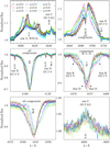 |
Fig. 2 Zoom-in of the nine available UVES spectra for various spectral lines (see legend). We note the antiphase motion of star B, the static RVs of star C, and the long-term RV variation of star D. |
3.1 Components A (WN3:h) and B (O5.5 V)
The WR primary (WN3:h, see Sect. 5.4) is easy to distinguish because of its rapidly moving emission lines (e.g., N V λλ4604, 4620 and He II λ4686, upper panels of Fig. 2), especially seen in the spectra taken close to opposite quadratures (ϕ = 0.20, 0.74). To look for the companion, we ought to identify features that portray an antiphase behavior compared to the WR star. Foellmi et al. (2003) identified such an antiphase motion in the Balmer lines owing to their high S/N, and used these lines to derive RVs for the companion. The antiphase motion in Hδ can be seen in the middle left panel of Fig. 2. It is evident that the RV amplitude of this line is relatively low (≈ 50 km s−1), which explains the high mass ratio obtained by Foellmi et al. (2003). However, as it turns out, the Balmer lines contain contributions from four stars (Sect. 3.2), making them unsuitable for accurate RV measurements.
The true companion of the WR star exhibits a much larger RV amplitude than derived by Foellmi et al. (2003). This can be seen when comparing the quadrature spectra in the middle right panel of Fig. 2, where the He I λ4471 line is shown (star B). One can notice that the ϕ = 0.74 spectrum exhibits a roundish absorption feature that is redshifted with respect to the line center. This same feature, somewhat less pronounced, becomes blueshifted in the ϕ = 0.20 spectrum. Star B is a rapidly rotating O-type star, which we later classify as O5.5 V (see Sect. 5.2). Companions A and B together make the 6.5 d-period WR binary in AB 6.
3.2 Components C (O5.5 I(f)) and D (O7.5 V)
Figure 2 reveals that additional components are present in the spectrum of AB 6. Star C, which contributes to all prominent spectral features, can be seen in emission lines that are apparently static (within errors), such as N III λλ4634, 4642 and N IV λ4060. These lines belong to neither star A nor star B because they do not follow their Doppler motion. For the same reason, these lines cannot originate in a wind-wind collision (WWC) cone (see Sect. 4.4). Hence, star C is an emission line star (O5.5 I(f), see Sect. 5.3) that displays little or no Doppler motion.
The fourth component, star D, can be easily seen in the Si IV λλ4089, 4116 doublet (middle left panel in Fig. 2), but also in He lines (mostly He I). This star, later classified as O7.5 V (Sect. 5.1), exhibits very narrow absorption features and significant RVs. However, neither the line profiles nor the RVs may be attributed to stars A, B, or C. For example, it is evident from Fig. 2 that star D remains almost static in the two quadrature spectra (ϕ = 0.74 and ϕ = 0.20), but shows a clear RV shift in another spectrum (ϕ = 0.10), which was taken ≈80 d after the quadrature spectra. A similar behavior can be seen in He I lines and to a lesser extent in the He II λ4686 line. In Sect. 6.3, we show that it is very likely that star D forms a second binary system with a fifth component that is not seen in our spectra, making AB 6 a quintuple system (Fig. 3).
4 Orbital analysis
4.1 RV measurements
To measure the RVs of the various components in the nine available UVES spectra, we employed a technique identical to that described in Shenar et al. (2017b). The method relies on cross-correlating the spectra with a template spectrum. If the line that is to be cross-correlated originates primarily in one component, the best template can be constructed by co-adding the observations in the frame of reference of this companion. However, to do so, one needs a first estimate for the RVs. This first estimate was obtained using preliminary model spectra (see Sect. 5).
For star A (WN3:h), we measured RVs for both the He II λ4686 and N V λλ4604, 4620 lines. The latter clearly offers a more reliable way of measuring the RVs. First, the sharply peaked N V profiles allow for a relatively accurate RV determination. Second, the N V lines form close to the stellar surface (r ≈ 1.5 R*) and their Doppler shift should therefore represent the motion of the WR star much more accurately than the He II λ4686 line. Third, the N V doublet is not contaminated by the other stars. We also measured the RVs of the N V λ4944 line. The values agree with the N V doublet within errors (see Fig. 10). Because of the relatively low S/N of the N V λ4944 line and normalization uncertainties, we adopted the N Vλλ4604, 4620 RVs for our orbital solution (see Sect. 4.2).
For star C (O5.5 I(f)), we used the isolated N IVλ4060 line, since itis not contaminated by the other stars and is relatively easy to cross-correlate with. Virtually identical RVs were obtained using the N III lines. For star D (O7.5 V), we used an average of the narrow Si IV λλ4089, 4116 lines. The same method cannot be easily applied to star B, since all its spectral features are contaminated by the other components. However, we took advantage of the fact that the RVs of the other components are known. For each of our nine spectra, we subtracted preliminary models for stars A, C, and D to isolate the contribution of star B. We then used the He I λ4471 and λ5875 lines for the cross-correlation, which have the advantage of not being contaminated by star A.
Once these estimates were obtained, we constructed four new templates by co-adding the observations in the frame of stars A, C, and D, respectively. These templates were used exactly as described above. The RVs obtained in this way were found to be in good agreement with the previous iteration, but the scatter was smaller. The derived RVs for the nine spectra and the four components are shown in Fig. 4 and are compiled in Table 1.
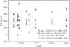 |
Fig. 4 Derived RVs for the components of AB 6 (see legend). |
4.2 Orbital solution for the WR binary (stars A+B)
Using the RVs measured for stars A and B, we can now derive an orbital solution for the system. For the WR component, we also make use of RVs measured by Moffat (1982), Hutchings et al. (1984), and Foellmi et al. (2003) for the He II 4686 line. Unfortunately, Foellmi et al. (2003) did not tabulate their measured RVs, so we extracted the RVs from Fig. 3 in their study using the Engauge Digitizer Software1, accounting for the systematic instrumental shifts reported in their work. With the full set of RVs, we derive an orbital solution using a self-written Python script, which uses the standard Python routine lmfit2. The routine fits both components simultaneously for the period P, time of inferior WR conjunction E0 (i.e., the WR star is in front the O star), RV amplitudes KWR and KO, eccentricity e, argument of periastron ω, and systematic velocity V0. Since deriving absolute RV values using emission lines is prone to significant systematic errors originating in the uncertain velocity law and mass-loss rate, we allow for a constant shift parameter for the RVs derived for the WR star. The shift parameter of the UVES measurements obtained from the final fit is given in the footnotes of Table 1
One concern is that the RVs from previous studies were measured using the He II λ4686 line. Since this line forms a few stellar radii above the stellar surface, it is more susceptible to distortions (e.g., WWCs, see Sect. 4.4) and is generally known to exhibit a strong variability that is both phase and epoch dependent (e.g., Foellmi et al. 2008; Koenigsberger et al. 2010). Therefore, we fit two orbital solutions. For both solutions, He I λ4471, 5875 are used for star B, but different lines are used for star A.
For the first solution, we use the He IIλ4686 line, combining old+new RVs. The solution (χ2 = 3.8 km s−1) is shown on the left panel of Fig. 5. A good agreement is obtained between the old and new measurements and enables an accurate derivation of the period, which is found to be P = 6.53840 d. However, it is also clear that a phase shift exists between the RVs of stars A and B, implying that the He II λ4686 line does not represent the true motion of the WR star. This is most likely a consequence of WWC (see Sect. 4.4).
As discussed above, the N V RVs should provide a better representation of the true motion of star A. For the second solution, we, therefore, fit the nine measured RVs of the N V doublet for star A simultaneously with star B. Because the period can be much better constrained using the He II λ4686 orbital solution, which covers ≈ 40 yr of data, we fix it to the value given above. We then use the measured N V RVs to fit for the remaining orbital parameters. The orbital fit is shown on the right panel of Fig. 5 and has a χ2 = 0.6 km s−1, which is six times better than obtained for the He IIλ4686 fit. This time, no phase shift is seen between the two components, suggesting that this solution represents the true orbital configuration of the system much better. Therefore, we adopt the orbital parameters obtained using the N V doublet. We note that the two solutions result in similar parameters, except for KWR, which is about 30 km s−1 larger in the He II solution. The final parameters are given in Table 2, along with values obtained by Foellmi et al. (2003) for comparison.
The period derived in this work agrees with previous derivations within 3σ. Since our derived value is based on data extending over 40 yr, it should be closer to the true period. The eccentricity is found to be smaller (0.03 ± 0.02) than previously reported, implying a virtually circular orbit. The RV amplitude of star B, KO, is found to be almost twice as large as previously reported. As a consequence, the mass ratio q = MO∕MWR diminishes from 4.4 to 2.2. Since only Msin3i can be derived from an orbital analysis, the orbital masses strongly depend on i. Foellmi et al. (2003) reported i = 65 ± 7° based on unpublished polarimetric data, but as this analysis was never published, it cannot be readily adopted.
In Sect. 4.3, we constrain i using the light curve of the system. However, our light-curve model is too crude to yield significant constraints on the orbital masses. Instead, given that the parameters of star B are fairly well known, we adopt its mass from calibration with evolution models. For this purpose, we use the BONNSAI3 Bayesian statistics tool (Schneider et al. 2014). The tool interpolates over evolutionary tracks calculated at SMC metallicity by Brott et al. (2011) for stars with initial masses up to 100 M⊙ and over a wide range of initial rotation velocities. Using the derived values for T*, log L, and log g, and their corresponding errors, BONNSAI predicts MO = 41 ± 5 M⊙. This is 4 M⊙ lower than the evolutionary mass of a star with the same parameters at solar metallicity, which is consistent with theoretical expectation (e.g., Markova et al. 2009; Garcia & Herrero 2013). This value agrees with the spectroscopic mass of star B, Mspec, within errors (which are very large). Considering the uncertainties involved in this approach, we conservatively adopt M2 = 41 ± 10 M⊙ for star B. This implies i = 53° and MWR = 18 M⊙. In Table 2, we also give the semimajor axes a and the Roche lobe radii RRL, calculated using the Eggleton approximation (Eggleton 1983).
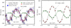 |
Fig. 5 Left panel: SB2 orbital solution for the WR binary in AB 6 (WR: black curve; O: green curve) using the complete set of RV measurements of the He II λ4686 line for star A and the He Iλ4471 line for star B (see legend). Right panel: same as left panel, but using the N V λλ4604, 4620 doublet RVsfor star A. See text for details. |
4.3 Light curve modeling
In Fig. 6, we show the I-band OGLE light curve of AB 6 (Udalski et al. 1998), phased with the ephemeris in Table 2. Two faint and broad dips can be seen during both conjunctions (ϕ = 0, 0.5). In principle, these could be grazing photospheric eclipses, wind eclipses, ellipsoidal variations, reflection effects, or even induced pulsations (e.g., Pablo et al. 2015).
At first, it seems that the two dips are suggestive of grazing eclipses. However, given the large temperature difference between stars A and B, the eclipse of the WR star (ϕ = 0.5) should be significantly more pronounced than that at ϕ = 0, which is not the case. Moreover, grazing eclipses should be relatively narrow, with Δ ϕ ≈ 0.05−0.1 (e.g., V444 Cyg, Antokhin et al. 1995), while the dips observed here spread over Δ ϕ ≈ 0.3. Lastly, given the orbital parameters and the radii derived from our spectral analysis (Sect. 5), grazing eclipses are only obtained for i > 73°, resulting in implausible masses of MO < 23 M⊙ and MWR < 10 M⊙. It therefore seems likely that other mechanisms are at work here.
A natural explanation for the dip at ϕ = 0 (WR star in front) are wind eclipses (Lamontagne et al. 1996; St-Louis et al. 2005). The relatively strong wind of the WR star can scatter the light from its companion, primarily via electron scattering. This can be modeled in a straight forward fashion by assuming a simple β law for the velocity field of the WR star and adopting the parameters derived in this study, including the mass-loss rate, which is derived in Sect. 5. The formalism has been thoroughly described in Lamontagne et al. (1996) and Munoz et al. (2017).
Yet wind eclipses cannot explain the dip observed around ϕ =0.5, as the wind of star B is too weak to lead to a significant eclipse. To investigate possible mechanisms that can reproduce this dip, we generated a light curve model using the Physics Of Eclipsing BinariEs 1.0 (PHOEBE) program (Prša & Zwitter 2005). While this program is robust, it does not include wind physics. However, it is still useful for determining plausible physical models that could influence the light curve. Using the parameters derived in Tables 2 and 3, our model light curves suggest that the dominant modulation is heating of the O star surface by the WR star, referred to as the reflection effect (Kopal 1954). When this heated up surface points toward the observer (ϕ = 0), excess emission is predicted, while an emission deficiency is predicted at ϕ =0.5 – exactly as observed. While this phenomenon is likely more complex in WR stars than our model is able to replicate, we are able to recreate both the shape and magnitude of the observed variation simply by adopting the parameters of the system, which lends credence to our rough approximations.
By interpolating over reflection models calculated with PHOEBE at various inclinations and combining this with the wind-eclipse model described above, we generate a combined Phoebe+wind-eclipse light curve model, which can be calculated at a given inclination i. All the relevant parameters except for the inclination are kept fixed, and the constant contribution of stars C and D is accounted for in the model. The best-fitting model, obtained for an inclination of i = 57°, is shown in Fig. 6. We also show the models for i = 45° and i = 65° for comparison. Since the wind eclipse at i = 65° overestimates the absorption at ϕ ≈ 0, we can rule out grazing eclipses in the system, as such eclipses would yield additional absorption to the wind eclipse. The formal error on i is ± 2°, but given all the assumptions involved in this model, this error is clearly underestimated. This result should be considered as a qualitative illustration of how reflection + wind eclipses can reproduce the main features of the light curve at an inclination that is consistent with the adopted value of i = 53°.
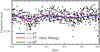 |
Fig. 6 Combined Phoebe + wind-eclipse light curve model calculated for three inclinations (i = 45°, 65°, and the best-fitting value 57°; see legend), compared to the OGLE light curve (unbinned and binned at Δ ϕ = 0.03). Formal errors in the unbinned light curve are comparable to the symbol sizes. |
4.4 Wind-wind collisions
When two stars in a binary possess strong stellar winds, the winds are expected to collide and form a shock cone around the companion whose mass loss is smaller (Stevens et al. 1992; Moffat 1998). The shocked material radiates in one or more spectral bands (X-rays, visual) as it streams along the cone, which corotates with the system. Some known examples for WWC systems are η Car (Parkin et al. 2009)and γ2 Vel (Richardson et al. 2017) in the Galaxy, HD 5980 in the SMC (Nazé et al. 2007), and BAT99 119 in the LMC (Shenar et al. 2017b). Unless the system is seen close to pole-on, and neglecting aberration and Coriolis forces, the emission from the WWC cone should become redshifted at ϕ =0 (the stream recedes away from the observer) and blueshifted at ϕ = 0.5 (e.g., Fig. 6 in Hill et al. 2000).
Evidence for WWC can be seen in Fig. 7, where a dynamical spectrum of the He II λ4686 line using the nine UVES observations is shown. We show both the original normalized spectra (left panel) and spectra from which the average contribution of the WR star, shifted to its respective RV, was subtracted (right panel). The average was constructed by co-adding the observations in the frame of reference of the WR star.
After subtracting the contribution of the WR star, a clear emission excess pattern is visible that is redshifted at ϕ =0 and blueshifted at ϕ = 0.5 (traced with a blue sine curve), exactly as expected in the case of WWC systems. With significant phase coverage, one can constrain kinematic information about the shock cone from such patterns (Luehrs 1997; Shenaret al. 2017b). However, with only nine observations and considering the quintuple nature of the system, this would not yield any meaningful constraints, and we therefore refrain from such an analysis.
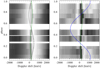 |
Fig. 7 Left panel: dynamical spectrum of the He IIλ4686 line in velocity space. The RV curves of stars A and B are shown. Right panel: same as left panel, but with the contributionof the WR star subtracted. The residual emission excess (traced with the blue curve) follows the expected behavior of a WWC cone. |
5 Spectral analysis
Phase-dependent spectra can be used to disentangle them from the constituent spectra (Hadrava 1995; Shenar et al. 2017b). We attempted to disentangle the UVES spectra using the shift-and-add technique (Marchenko et al. 1998), which we extended for the case of four components. The results are shown in Fig. 8. While the disentangled spectra are plausible for most spectral lines, the Balmer lines and strong He II lines (especially λ4686) are poorly constrained. We, therefore, do not rely on these disentangled spectra for the spectral analysis. However, the disentangled spectra enable us to spectroscopically classify the components. We use classification schemes by Smith et al. (1996) for star A, and quantitative classification schemes by Sana et al. (in prep.), which are extensions of schemes by Mathys (1988, 1989), Walborn & Fitzpatrick (1990), and Walborn et al. (2002) for stars B and D. Star C is classified morphologically using Massey et al. (2009). Details are given in Sects. 5.1–5.4. Thankfully, important spectral features can be unambiguously attributed to each component (Fig. 2). The spectral analysis thus virtually reduces to the analysis of four single stars with the exception of the unknown light ratios.
The spectral analysis is performed with the Potsdam Wolf-Rayet4 (POWR) model atmosphere code (Gräfener et al. 2002; Hamann & Gräfener 2004), which is applicable to any hot star (e.g., Gvaramadze et al. 2014; Giménez-García et al. 2016). The code iteratively solves the comoving frame, nonlocal thermodynamic equilibrium (non-LTE) radiative transfer and statistical balance equations in spherical symmetry under the constraint of energy conservation, yielding the population numbers in the photosphere and wind. By comparing output synthetic spectra to observed spectra, fundamental stellar parameters are derived. A detailed description of the code is given by Gräfener et al. (2002) and Hamann & Gräfener (2004). Only essentials are given here.
Aside from the chemical abundances and the wind velocity field, a PoWR model is defined by four fundamental stellar parameters: the effective temperatureT*, stellar luminosity L, mass-loss rate Ṁ, and surface gravity g*, the latter being seldom important for WR stars. The effective temperature is defined at the stellar radius R* via the Stefan-Boltzmann equation  . The stellar radius is defined at the inner boundary of the model, fixed at Rosseland mean optical depth of τRoss = 20. The outer boundary is set to Rmax = 1000 R*. The gravity g* relates to the radius R* and mass M* via the usual definition,
  .
.
The PoWR models include complex model atoms of H, He, C, N, O, Mg, Si, P, S, and the iron group elements dominated by Fe. Abundances that cannot be derived from the spectra are fixed based on studies by Korn et al. (2000), Trundle et al. (2007), and Hunter et al. (2007), which are (in mass fractions) XH = 0.73, XC= 2.1 × 10⁻⁴, XN= 3.26 × 10⁻⁵, XO= 1.13 × 10⁻³, XMg = 9.9 × 10⁻⁵, XSi = 1.3 × 10⁻⁴, and XFe = 3 × 10⁻⁴. The remaining elements are scaled to 1/7 solar: XP = 8.3 × 10⁻⁷ and XS = 4.4 × 10⁻⁵.
Quasi-hydrostatic equilibrium is assumed in the subsonic regime (Sander et al. 2015), while a β law (Castor et al. 1975),
 (1)
(1)
is assumed for the supersonic regime. Here, β is a constant on the order of unity, v∞ is the terminal velocity, and r0 is a constant chosen so that a smooth transition between the sub- and supersonic regimes is obtained. We adopt β = 0.8 for OB-type models (Kudritzki et al. 1989). For the WR-star model, we adopt a two-component β law (see Sect. 5.4).
During the main iteration of the PoWR code, the opacity and emissivity profiles are calculated with a constant Doppler width of vDop = 30 km s−1 for OB-type stars and 100 km s−1 for the WR star. In the calculation of the emergent spectrum in the observer’s frame, vDop is calculated from the microturbulence and thermal motion via  . The microturblence grows from its photospheric value ξph in proportion to the wind velocity as ξ(r)= 0.1 v(r). The value ξph is set to 20 km s−1 for stars B and C, 100 km s−1 for star A, and ξph= 3 km s−1 for star D (see Sect. 5.1).
Optically thin clumps are accounted for using the microclumping approach (Hillier 1984; Hamann & Koesterke 1998), where the population numbers are calculated in clumps that are a factor of D denser than the equivalent smooth wind. We find D = 10 provides a good agreement in all cases, and refrain from fitting this parameter. The stratification of clumps is not well constrained. Some studies suggest that clumping initiates slightly above the stellar surface at r ≈ 1.1 R* because of line-driven instability (Owocki et al. 1988; Feldmeier et al. 1997), while other studies suggest that clumps already originate in subphotospheric layers (Cantiello et al. 2009; Ramiaramanantsoa et al. 2018). We assume D = 1 at the photosphere, which reaches its maximum value D = 10 at r = 1.1 R*. The detailed form of the stratification may have some effect on the line profiles, but does not significantly affect our results. In this study, we ignore the effect of optically thick clumps or macroclumping (Oskinova et al. 2007; Šurlan et al. 2013). While potentially important, high quality, phase dependent UV data are necessary to obtain constraints on the clump geometry. Overall, accounting for macroclumping can introduce an increase of up to a factor of  in the derived mass-loss rate (e.g., Oskinova et al. 2007; Shenar et al. 2015).
Because optical WR spectra are dominated by recombination lines, whose strengths increase with  , it is customary to parametrize their models using the so-called transformed radius,
![Mathematical equation: \begin{equation*} R_{\text{t}} = R_* \left[ \frac{v_{\infty}}{2500\,\textrm{km}\,\textrm{s}^{-1}\,} \middle/ \frac{\dot{M} \sqrt{D}}{10^{-4}\,M_{\odot}\,\textrm{yr}^{-1}} \right]^{2/3}\vspace*{2pt}\end{equation*}](/articles/aa/full_html/2018/08/aa33006-18/aa33006-18-eq7.png) (2)
(2)
(Schmutz et al. 1989), defined so that equivalent widths of recombination lines of models with given abundances, T*, and Rt are approximately preserved, independent of L, Ṁ, D, and v∞.
In principle, the temperatures are derived from the ionization balance of different species, gravities from the strengths and shapes of Balmer lines, and wind parameters from wind lines (Hα, He II λ4686, UV resonance lines). The projected rotational velocity veq sini is derived by convolving the models with appropriate rotation profiles. For the WR and O(f) components (stars A and C), we applied a 3D integration routine (Shenar et al. 2014) to derive veq sini from emission lines. We account for macroturbulence by convolving the model spectra with radial-tangential profiles with vmac = 20 km s−1 (Gray 1975; Simón-Díaz & Herrero 2007; Puls 2008). Abundances are derived from the strengths of corresponding spectral lines. The synthetic composite spectrum is convolved with Gaussians to mimic the instrumental profiles of the observations. The models of stars A and B also account for Auger ionization via X-rays (Baum et al. 1992).
The total luminosity log Ltot and reddening EB−V are derived by fitting the total model flux to the observed SED. The reddening is modeled using a combination of reddening laws derived by Seaton (1979) for the Galaxy and by Gordon et al. (2003) for the SMC, where EB−V = 0.03 is assumed for the Galaxy and the total-to-selective extinction is set to RV = 3.1.
The most challenging part is determining the light ratios simultaneously with the mass-loss rate of the WR star. This is because an increase of the mass-loss rate of the WR star can be compensated for by decreasing the contribution of the WR star to the total visual light, thereby inducing a stronger dilution of its lines. The problem was solved iteratively, constraining first components whose light contribution is easier to establish. Details regarding the analysis are given in Sects. 5.1–5.4.
The global fit to the data at ϕ ≈ 0.1 is shown in Fig. 9. A fit to specific lines at five different phases is shown in Fig. 10. The derived stellar parameters are given in Table 3, where we also give the equatorial rotation velocity veq, absolute visual magnitude MV, light ratio in the V band fV ∕fV, tot, and number of H-ionizing photons log Q. Spectroscopic masses are calculated from g* and R*. Errors on fundamental parameters follow from the sensitivity of the fit to their variation (see details below). The remaining errors are calculated via error propagation.
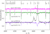 |
Fig. 8 Disentangled spectra of stars A, B, C, and D, shifted to their relative contribution in the visual. With only nine observationsand given the four stellar components, the reproduced strengths of the Balmer lines and important He lines are poorly constrained and should not be considered as real. |
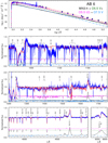 |
Fig. 9 Upper panel: comparison between observed photometry and flux-calibrated IUE and FUSE spectra (blue squares and lines) with the best-fitting model SED of AB 6 (red dotted line), which is the sum of the reddened SEDs of stars A, B, C, and D (black solid, green dotted, pink dashed, and cyan dot-dashed lines). Lower panels: comparison between normalized FUSE, IUE, and UVES spectra at ϕ ≈ 0.1 and the best-fitting normalized spectrum of AB 6, comprising the weighted models of stars A, B, C, and D. Line styles are as in the upper panel. |
Derived parameters from the spectral analysis of AB 6.
5.1 Star D (O7.5 V)
Despite its faintness, star D is the easiest to model. Given its relatively low temperature, it exhibits lines that are not present in any of the other stars, such as the Si IVλλ4089, 4116 doublet, and weak He I lines. Moreover, its line profiles are very narrow and easy to distinguish from the other components (see Fig. 2). A weak signature of this star is also visible in strong He II lines, which enabled us to derive its temperature from the He II/I balance and the ionization balance of N and O lines. A peculiarity of star D is its extremely narrow spectral lines, which could only be reproduced assuming ξph ≤ 3 km s−1 and veq sini ≤ 3 kms. This result is reminiscent of the very low rotation and turbulence measured for the magnetic O9.7 V star HD 54879 (Shenar et al. 2017a), raising the possibility that star D may be a magnetic star.
With the temperature fixed, the light ratio of star D could be well constrained based on the strengths of its spectral lines, assuming no abnormal abundances, and is found to be 10%. Deriving log g* for star D proved to be very difficult because the Balmer lines contain contributions from all components. Given its derived luminosity and its stellar parameters, star D is very likely a main sequence star, and so log g* was taken with an appropriate value for late-type OB main sequence stars (≈ 4.0 [cgs]). The value is consistent with the data within ≈0.3 dex.
The wind parameters of star D could not be constrained owing to its faintness. A terminal velocity of v∞ = 2000 km s−1 is adopted based on scaling relations with the escape velocity (Leitherer et al. 1992). The mass-loss rate was fixed to log Ṁ = −9.4 (M⊙ yr−1), which is based on the typical mass-loss rates of late-type O stars (e.g., Bouret et al. 2003; Marcolino et al. 2009; Shenar et al. 2017a) scaled down with Z0.7 (Vink et al. 2001).
5.2 Star B (O5.5 V)
While all spectral lines of star B are entangled with the other components, their round profiles make star B easily recognizable in strong He lines (see Figs. 2 and 10). The ionization balance of He was the main criterion for deriving T* for star B, which is found to be 41.5 kK. We derive veq sini = 210 km s−1, which is significantly higher than average (e.g., Ramírez-Agudelo et al. 2013), potentially due to past mass transfer (e.g., de Mink et al. 2013; Shara et al. 2017; Vanbeveren et al. 2018, see Sect. 6.2). With these parameters fixed, the relative contribution of star B to the visual flux could be derived from the strength of the He lines assuming normal abundances.Star B is estimated to contribute 36% in the visual. The gravity cannot be accurately derived, but log g* = 4.0 (cm s−2) is consistent with the data within 0.3 dex, which suggests that star B is a main sequence star. The disentangled spectrum of star B is intermediate between O5 and O6, which led tothe final estimate of O5.5 V.
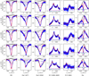 |
Fig. 10 Phase-dependent fits for various phases and spectral lines (see axes labeling). Line styles are as in Fig. 9. |
5.3 Star C (O5.5 I(f))
Star C is most easily seen in apparently static N III and N IV emission lines. However, it also contributes significantlyto strong He I and He II lines (see Fig. 10), which aids in constraining T*. To obtain N III and N IV in strong emission, log g* are necessary. The value veq sini could be derived based on both the weak emission lines of the star, which are formed very close to its photosphere, and from He I absorption lines. The light ratio is determined from the overall strength of the He lines; the N lines are not helpful in this case because the N abundance of O(f) stars is uncertain. Star C is found to contribute roughly 45% of the total visual light. After fixing its light ratio, the nitrogen abundance of star C could be constrained and is found to be ≈ 20 times the SMC average (see Table 3), which agrees with it being an evolved supergiant star. The disentangled spectrum of star C shows great similarity to the O5.5 I(f) star AzV 75 in the SMC (Massey et al. 2009), whose spectral type we therefore adopt.
5.4 Star A (WN3:h)
Finally, with the parameters of stars B, C, and D fixed, the parameters of star A can be derived. The previously derived light ratios imply that star A contributes about 9% to the total visual light. With only N V lines present among the nitrogen lines in the optical spectrum, we can conclude that the temperature of the WR star has to be larger than 75 kK. A good agreement is obtained for 80 kK. In principle, T* can be arbitrarily larger, placing the star in the so-called T*−Rt degeneracy domain (Hamann et al. 2006). However, at significantly larger values of T* (> 90 kK), the N V doublet forms further out in the wind and the line profiles become broad and smeared unlike the sharply peaked profiles observed. Admittedly, the line profiles are sensitive to the adopted velocity law and clumping stratification. We, therefore, conservatively adopt a large upper bound on T*. Correspondingly, Rt has a large lower bound. Nevertheless, the error on Ṁ remains relatively small because models of similar line strengths in the degeneracy domain maintain similar values of Ṁ. A physical reason to prefer a lower T* is that higher temperatures generally require higher luminosities to reproduce the same observed flux, which only worsens the Eddington- limit problem.
The gravity of the WR star has virtually no impact on its spectral appearance and is therefore not fitted here, but kept fixed to the value implied from the orbital mass and stellar radius of the WR star. With the temperature and light ratio fixed, the mass-loss rate and detailed abundances immediately follow from the strengths of the emission lines in the spectrum. Accounting for the four visible components implies that the luminosity of the WR star is smaller than previously derived by Shenar et al. (2016) and drops from log L = 6.3 to 5.9 [L⊙].
The nitrogen abundance is found to be five times larger than what is expected from the CNO cycle equilibrium (XN = 0.0015, e.g., Crowther 2007; Hainich et al. 2015). While the total error on XN may reach afactor of two due to uncertainties in the velocity law and clumping stratification, a mere inspection of the spectrum of star A in Fig. 8 suffices to indicate that it exhibits strong N V lines. Larger-than-expected XN is reported for all SMC WN stars (Hainich et al. 2015; Shenar et al. 2016). For example, the WN3ha star AB 12 was reported to have XN= 0.009 (Hainich et al. 2015). One way to enhance XN is by mixing carbon from the He-burning core into the H-burning shell, which is then converted to N during the CNO cycle (e.g., Vincenzo et al. 2016). Such a process could be supported by tidally induced mixing (e.g., Song et al. 2013). Another possibility is that the original CNO abundance was larger than the SMC average. Forexample, the derived abundances of star C are suggestive of a total CNO abundance that is ≈ 5% of the total stellar mass, i.e., three times larger than expected. Generally, derived XN values for SMC WR stars show quite a spread, a fact which should be investigated in future studies.
Foellmi et al. (2003) attributed the N IVλ4060 line to the WR component instead of star C. Star A seems to exhibit only N V lines in the optical, which, following Smith et al. (1996), implies the spectral type WN2h. However, as its spectrum is heavily diluted by the other components, we cannot exclude the presence of faint N IV or C IV lines associated with it. The disentangled spectrum of star A, with its enhanced S/N of ≈300, is suggestive of a very faint and broad N IV feature, but this could also arise from normalization issues. We therefore classify star A as WN3:h (“:” stands for uncertain).
The simple β law in Eq. (1) did not provide a good fit to the sharply peaked profiles of the N V lines (see Fig. 2). A better fit is obtained using an extension of the β law, dubbed the two-component β law (Hillier & Miller 1999; Todt et al. 2015), where a term similar to the standard β law is added to Eq. (1). We find that β1 = 1 and β2 = 4, which has a fractional contribution of 0.4 for the β = 4 component, provides a good fit to the N V lines. Larger β2 values of ≈10 (e.g., Lépine & Moffat 1999) result in line profiles that are too narrow in all emission lines. Future studies will try to consistently model the velocity field of the WR star in light of its known orbital mass and luminosity (Sander et al. 2017).
5.5 Atmospheric eclipses in the UV
The terminal velocities are based in part on IUE and HST UV spectra available here. Two HST spectra of the C IV λλ1548, 1551 resonance doublet taken close to inferior and superior WR conjunctions (ϕ = 0, 0.5) are shown in Fig. 11. The spectra show significantly more absorption when the WR star is in front of the O star (ϕ = 0) compared to when the O star is in front of the WR star (ϕ = 0.5). This, as well as the behavior of the N Vλλ1239, 1243 resonance doublet, was interpreted by Hutchings et al. (1993) as mutual irradiation effects of the winds of the WR star and its O companion. However, the latter authors were not aware of the two additional components in the system. In fact, the C IV resonance doublet is very robust and is not sensitive to the ionization structure except for very extreme X-ray irradiation effects.
We wish to offer a somewhat simpler and, we believe, more plausible interpretation for the changing absorption strength of the C IV resonance doublet. When the WR star is in front of the O star (ϕ = 0), the part of its wind that occults the O star leads to additional absorption along the line of sight toward the disk of the O star. This absorption occurs for Doppler shifts that lie within the minimum and maximum projected velocity of the wind that occults the O star. Given the orbital parameters, this should be slightly below the terminal velocity of the WR star. The absorption should occur both at redshifted and blueshifted wavelengths. This is exactly what is observed in the HST spectra. An accurate modeling of this requires the calculation of the non-LTE radiative transfer in nonsymmetric geometry, which is beyond the scope of this paper. With more UV observations covering the orbital phase, much better constraints on the mass loss of the primary and secondary could be obtained.
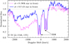 |
Fig. 11 HST spectra at ϕ ≈ 0 (pink line) and 0.5 (blue line) in velocity space relative to the blue component of the C IV doublet corrected for the systemic velocity V0 = 196 km s−1. |
6 Discussion
6.1 Eddington limit problem
One of the primary motivations for our study was the fact that the WR primary in AB 6 was found by Shenar et al. (2016) to exceed its expected luminosity by more than an order of magnitude, violating even the Eddington limit (see Fig. 1). We now consider this problem in light of the new parameters derived in this study. In Fig. 12, we plot a revised version of the M−L diagram shown in Fig. 1, but include the newly derived parameters for star A. We also plot mass-luminosity relations calculated for homogeneous stars with different hydrogen contents by Gräfener et al. (2011).
Since MWR derived in this work is roughly a factor of two larger than the value reported by Foellmi et al. (2003), and the luminosity is about 0.4 dex lower than the value reported in Shenar et al. (2016), the WR primary is located below, yet close to, the Eddington limit (Fig. 12), with an Eddington Gamma of ΓEdd = 0.8. The urgent Eddington limit problem is therefore resolved via new, high quality UVES observations. The WR primary is still found to be overluminous compared to its respective homogeneous relation (with XH= 0.25), implying that it is not homogeneous but rather core He burning and shell H burning. A similar result was obtained for most WR binaries in the SMC (Shenar et al. 2016).
Considering the relatively stable behavior of the WR component, its proximity to the Eddington limit is still surprising, especially when considering the full radiative force, which also accounts for line transitions. According to our model, the additional line acceleration in the deep quasi-hydrostatic layers because the Fe opacity peak causes the total outward force to exceed gravity, implying an unstable configuration. Similar results were obtained by Gräfener& Hamann (2008). Given recent theoretical work on stellar envelope inflation in WR stars (e.g., Gräfener et al. 2011; Sanyal et al. 2015; Grassitelli et al. 2018), it is possible that, while our model accurately describes the conditions in the wind of the WR star, it does not do so for its deep layers. However, this should have no bearing on our results.
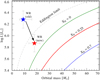 |
Fig. 12 As in Fig. 1, but including the new position of star A. Apart from the Eddington limit (dashed gray line), we also plot mass-luminosity relations calculated for homogeneous stars with various hydrogen contents (see labeling). |
6.2 Evolutionary context
Since stars A+B (WN3:h+O5.5 V) constitute a close binary, they likely interacted in the past (and will probably do so in the future). Modeling their evolution therefore needs to account for binary interaction. Here, we use a grid of binary tracks calculated with the BPASS5 (Binary Population and Spectral Synthesis) stellar evolution code (Eldridge et al. 2008, 2017) calculated for Z = 0.004 to find a suitable evolutionary channel of the system.
Each binary track is defined by a set of three parameters: the initial mass of the primary Mi,1, the initial mass ratio qi = Mi,2∕Mi,1 < 1, and the initial orbital period Pi. The tracks are calculated at a spacing of 0.2 dex on 0 < log P [d] < 4, a spacing of 0.2 on 0 < qi < 0.9, and an uneven spacing of ≈0.05−0.1 dex on Mi,1, amounting to roughly 6000 tracks. To find the best-fitting track and a corresponding age t, we minimize
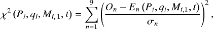 (3)
(3)
where 
 are the measured values for the considered observables, and
  are the predictions of the evolutionary track defined by Pi, qi, and Mi,1 at time t. σn is defined by
 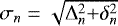 , where Δn is half the n’th parameter’s grid spacing, and δn is the formal fitting error (see Tables 2 and 3).
The best-fitting track is found to be that calculated with the initial parameters Mi,1 = 60 M⊙, qi = 0.7, and Pi = 16 d at an age of 3.9 Myr. Roche-lobe overflow (RLOF) is predicted to have taken place shortly after core hydrogen exhaustion (case B mass-transfer; Kippenhahn & Weigert 1967) for ≈ 30 kyr, during which about 20 M⊙ were lost from the primary and 5 M⊙ were accreted by the secondary. The tracks for the primary and secondary companions are shown in Fig. 13. We also show a single-star track calculated by Eldridge et al. (2008) for an initial mass of Mi = 60 M⊙ for comparison. In Table 4, we compare the observables On to the prediction by the best-fitting binary track En, also stating the uncertainty σn used in Eq. (3). It is evident from Fig. 13 and Table 4 that the binary track does very well in reproducing the observed parameters of the system.
The tracks used in this work assume no initial rotation and do not perform a detailed evolution of the angular momentum of the system. Rapid initial rotation may cause the stars to undergo quasi-homogeneous evolution (QHE), avoiding expansion and, correspondingly, mass transfer in the system (Maeder & Meynet 2003). While studies point out that initial rotation velocities, at least for O-type binaries, are unlikely to take near-critical values (Ramírez-Agudelo et al. 2013, 2015), this cannot be ruled out in specific cases. For example, there is compelling evidence that the massive WR binary SMC AB 5 (HD 5980) evolved via QHE (Koenigsberger et al. 2014; Shenar et al. 2016). To test this channel, we investigated a set of BPASS tracks calculated for homogeneous stars (Eldridge et al. 2011)for a solution that best fits the observed properties of the WR component. The best-fitting track, found for Mi = 40 M⊙, is shown in Fig. 14. This track never exceeds a radius of 9 R⊙, remaining well within the current Roche radius of the WR star (see Table 2), which was likely not smaller in the past. Therefore, if QHE indeed characterizes the evolution of the system, the binary components would have avoided interaction. In this case, apart from tidal effects, their evolution can be modeled as for isolated single stars.
The best-fitting homogeneous track for the WR star implies an age of 6.3 Myr, which is roughly twice the age derived assuming binary evolution. Itis evident from Fig. 14 that QHE cannot reproduce the hydrogen content of the WR star, with the track predicting XH = 0 at its observed HRD location. The current stellar mass predicted by the track is 30 M⊙, showing a larger deviation from our 18 M⊙ measurement compared to the binary evolution track. However, the most severe issue is reproducing simultaneously the observed parameters of the O companion. To test whether QHE is consistent with the evolutionary status of the secondary, we use the BONNSAI tool. Using T*, L, Morb, veq derived for the secondary and the age derived for the WR star under the QHE assumption (6.3 Myr), the algorithm tests whether a model exists that can reproduce the properties of the secondary at a 95% significance level. The results are conclusive: no solution can be obtained for the secondary. This result could be anticipated since the initial mass of the secondary would have to have been smaller than the 40 M⊙ of the primary, although its current mass is estimated at 41 M⊙. Moreover, after 6.3 Myr, the O companion should be seen at an evolved stage, which is not observed. We can almost certainly reject QHE in the case of AB 6. We conclude that the system exchanged mass in the past. This is supported by the higher-than-average rotation velocity found for star B, on par with Galactic candidates of spun up companions in WR binaries (Shara et al. 2017).
It is interesting to note that while our results suggest that the WR star in AB 6 originally lost mass via RLOF, it is not clear that this mechanism was necessary for it to enter the WR phase. This can be easily seen in Fig. 13, which shows that a single star with Mi = 60 M⊙ is also predicted to become a WR star by the BPASS tracks. This prediction strongly relies on the mass-loss prescription adopted by the BPASS code. However, mass loss is still considered to be poorly understood, especially in light of stellar eruptions (e.g., Smith & Owocki 2006). A similar result was obtained in Shenar et al. (2016) for the other WR binaries in the SMC. This gives further evidence for the apparent lack of intermediate-mass WR stars that form via binary interaction (initial masses 10− 40 M⊙), which are expected to be abundant (Bartzakos et al. 2001; Foellmi et al. 2003).
In the discussion of the evolution of the system, we fully ignored stars C and D. In principle, additional companions can affect the evolution of a binary (e.g., Toonen et al. 2016). However, these effects cannot be considered until more information is collected on stars C and D (see Sect. 6.3).
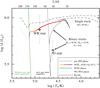 |
Fig. 13 Best-fitting BPASS binary track for AB 6, calculated for Mi = 60 M⊙, qi = 0.7, and Pi = 16 d. The upper multi-colored track depicts the evolution of the WR primary until its core-collapse. The colors refer to surface hydrogen mass fractions of 0.45 < XH < 0.7 (blue), 0.2 < XH < 0.45 (red), 0.05 < XH < 0.2 (orange), and XH < 0.05 (green). The WC and RLOF phases are also marked. A track for a single 60 M⊙ star is shown for comparison (dashed gray line). The lower track depicts the evolution track of the O-type companion until the core collapse of the primary. |
Derived parameters for the WR binary (On) compared to predictions by the best-fitting binary track (En).
 |
Fig. 14 As in Fig. 13, but depicting the best-fitting homogeneous evolution track calculated for a single Mi = 40 M⊙ star. The nonhomogeneous equivalent is shown for comparison (dashed line). |
6.3 Nature of stars C and D
A preliminary SB1 orbital fit to the measured RVs of start D is shown in Fig. 15. The resulting parameters are P = 139.1 d, V0 = 181 km s−1, K = 49 km s−1, ω =64°, e = 0.46, and T0 = 51937.3 [MJD]. For meaningful errors, more observations are necessary, preferably taken near periastron. Regardless, it is clear that star D orbits a massive object with a period on the orderof 100 d.
The first possibility is that star D orbits the WR binary, forming an hierarchical triple system. Adopting the spectroscopic mass derived for star D, the period derived above and the masses of stars A and B imply a separation of ≈ 500 ± 50 R⊙ between star D and the WR binary. Is such an orbit stable? Analytical stability criteria by Mardling & Aarseth (1999) suggested that, for the orbital parameters derived above, the orbit would be unstable for separations smaller than 450 ± 100 R⊙ (cf. Eq. (23)in Toonen et al. 2016). The stability condition is therefore only marginally fulfilled, and while we cannot rule out that star D revolves around the WR binary in a 140 d period, this configuration seems unlikely.
The only alternative is that star D forms a second binary. The most obvious candidate for a companion to star D would be star C. However, the RVs derived for star C are not consistent with it forming a binary with star C. We cannot detect any significant RV variability for star C within the 10 km s−1 error, and no antiphase trend is seen for the derived values (cf. Table 1 and Fig. 4). Figure 16 illustrates the long-term motion of star D in the Si IV λ4089 line, whose RV changes by ≈ 65 km s−1 within ≈80 d. For comparison, we also plot the N IVλ4060 line that originates in star C. No antiphase motion relative to star D is seen. If the companion is truly star C, we would expect an antiphase RV change whose amplitude scales with the mass ratio MD ∕MC. Assuming MD ≳ 20 M⊙ and nondetectability for an RV change smaller than 10 km s−1, the mass of star C would have to be
 (4)
(4)
which is very high and, while not impossible for an O(f) star, is not consistent with the luminosity and spectroscopic mass derived in this study for star C.
The preliminary orbital parameters for star D imply a mass function of f = 1.3 M⊙. Denoting the companion of star D with the letter X, a lower limit for the mass of the companion of star D can be obtained by solving the following cubic inequality:
 (5)
(5)
which yields MX > 11 M⊙. Hence, the companion of star D has to be a massive star (earlier than B3 V), for which there are three alternatives. The first option is that the companion of star D is star C and that MC > 130 M⊙ (see Eq. (4)). However, this is not favored, as argued above. The second option is that the companion of star D is a very faint early B-type star. A B2 dwarf would fulfill M > 11 M⊙ and would have an absolute visual magnitude of MV ≈− 2.5 mag (Schmidt-Kaler 1982), which may fall below our detection limit. The third option is that the companion is a massive black hole (BH). Using the parameters of star D from Table 3 and adopting the minimum mass of 11 M⊙ for a hypothetical BH on a circular orbit, Bondi-Hoyle accretion (Bondi & Hoyle 1944) would imply an X-ray luminosity of ~ 1031 erg s−1, which is negligible compared to WWC X-ray emission (Guerrero & Chu 2008). Hence, the presence of a BH cannot be ruled out by existing X-ray observations of this system.
To conclude, we suggest that the most likely configuration of AB 6 is a quintuple system, in which stars A+ B form the 6.5 d WR binary, star C a single star, and star D forms a second binary with either a BH or a B2 V star (Fig. 3). It remains unclear whether stars C, D, and the putative companion of star D are gravitationally bound to the A+B WR binary. Our results suggest that V0,A+B = 196 ± 4 km s−1, V0, C = 211 ± 4 km s−1, and V0, D+X = 181 ± 9 km s−1, although these errors (especially of stars C and D) may be well underestimated owing to systematics. Considering the errors, a gravitationally bound quintuple system can be neither confirmed nor ruled out. Since AB 6 is seen as a point source in our UVES exposure at a seeing of FWHM = 1.4″, and assuming no (extremely unlikely) line-of-sight contamination, we can estimate that the five components should be confined within a circle with a radius of ≈0.2 pc at the SMC distance. To know whether the system is gravitationally bound, more spectra of AB 6 are needed to further constrain the orbit of star D, and high resolution images of the immediate surroundings of AB 6 (e.g., HST, adaptive optics) may help to spatially resolve this important system.
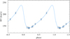 |
Fig. 15 Preliminary SB1 orbital solution derived for star D. |
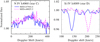 |
Fig. 16 Two UVES observations (MJD = 57944.4 58025.2 − 57944.4) that correspond to the maximum RV of star D. The left panel shows the N IV λ4060 line that belongs to star C, and the right panel shows the Si IVλ4089 line that belongs to star D. No antiphase motion can be seen in the spectrum of star C. |
7 Summary
This study presented new, high quality UVES observations of the shortest period SMC WR binary, SMC AB 6. The very low orbital massand high luminosity of the WR component reported in the past suggested that it exceeds the Eddington limit (Shenar et al. 2016). Our study aimed at understanding these peculiar results and investigating the evolutionary history of this system. To achieve this, we performed an orbital, light-curve, and spectral analysis, and compared our results to evolutionary tracks calculated with the BPASS code. We conclude the following:
True members of the WR binary resolved: the WR binary comprises an WN3:h component (star A) and a relatively rapidly rotating (veq = 265 km s−1) O5.5 Vcompanion (star B), orbiting each other at a period of 6.5 d. The new orbit derived implies MWR = 18 M⊙, which is twice the value reported in the past.
AB 6 is a quadruple or quintuple system: the presence of an emission-line O5.5 I(f) star (star C) and of a narrow-line, fainter O7.5 V star (star D) can be clearly seen in the spectrum. The RVs of star D suggest that it belongs to a second binary. The lack of opposite RVs for star C suggests that star D orbits a BH or a B2 V star. To know whether these additional components are gravitationally bound to the WR binary, more observations are needed.
Eddington limit puzzle resolved: the newly derived luminosity (log L = 5.9 [L⊙]) and orbital mass (18 M⊙) of the WR component no longer place it above the Eddington limit, although it remains significantly overluminous compared to a homogeneous star with the same hydrogen content.
Evidence for mass transfer: the properties of the WR binary can be well reproduced assuming that this binary originates in a system with initial masses Mi,1,2 = 60, 40 M⊙ and an initial period of Pi ≈ 16 d. The system very likely experienced mass transfer via RLOF in the past, with about 20 M⊙ lost from the primary and 5 M⊙ accreted by star B during RLOF. This is supported by the relatively rapid rotation of star B. The age of the system is estimated at 3.9 Myr. However, according to the same set of evolution tracks, any 60 M⊙ star would eventually reach the WR phase, regardless of binary interaction.
It appears that while the new UVES observations have answered decade-long questions related to this unique and important system, they also create new questions. How many more components will we find with new data? This study comes to show that our understanding of massive stars is strongly dependent on our capability of resolving them and coping with their multiplicity. We encourage new observations of this system to understand the nature of stars C and D, and their potential role in the evolutionary history of this unique WR multiple system.
Acknowledgements
We thank our referee, Paul Crowther, for helping to improve our manuscript. Based on observations collected at the European Organization for Astronomical Research in the Southern Hemisphere under ESO programme 099.D-0766(A) (P.I.: T. Shenar). T.S. acknowledges support from the German “Verbundforschung” (DLR) grant 50 OR 1612. V.R. is grateful for financial support from Deutscher Akademischer Austauschdienst (DAAD), as a part of Graduate School Scholarship Program. A.M. is grateful for financial aid from NSERC (Canada) and FQRNT (Quebec). L.M.O. acknowledges support by the DLR grant 50 OR 1508. A.S. is supported by the Deutsche Forschungsgemeinschaft (DFG) under grant HA 1455/26. This research made use of the VizieR catalog access tool, CDS, Strasbourg, France. The original description of the VizieR service was published in A&AS 143, 23. Some data presented in this paper were retrieved from the Mikulski Archive for Space Telescopes (MAST). STScI is operated by the Association of Universities for Research in Astronomy, Inc., under NASA contract NAS5-26555. Support for MAST for non-HST data is provided by the NASA Office of Space Science via grant NNX09AF08G and by other grants and contracts.
References
- Almeida, L. A., Sana, H., Taylor, W., et al. 2017, A&A, 598, A84 [NASA ADS] [CrossRef] [EDP Sciences] [Google Scholar]
- Antokhin, I. I., Marchenko, S. V., & Moffat, A. F. J. 1995, in, Wolf-Rayet Stars: Binaries; Colliding Winds; Evolution, eds. K. A., van der Hucht, & P. M., Williams, IAU Symp., 163, 520 [NASA ADS] [Google Scholar]
- Azzopardi, M., & Breysacher, J. 1979, A&A, 75, 120 [NASA ADS] [Google Scholar]
- Bartzakos, P., Moffat, A. F. J., & Niemela, V. S. 2001, MNRAS, 324, 18 [NASA ADS] [CrossRef] [Google Scholar]
- Baum, E., Hamann, W.-R., Koesterke, L., & Wessolowski, U. 1992, A&A, 266, 402 [NASA ADS] [Google Scholar]
- Bonanos, A. Z., Lennon, D. J., Köhlinger, F., et al. 2010, AJ, 140, 416 [NASA ADS] [CrossRef] [Google Scholar]
- Bondi, H., & Hoyle, F. 1944, MNRAS, 104, 273 [NASA ADS] [CrossRef] [Google Scholar]
- Bouret, J.-C., Lanz, T., Hillier, D. J., et al. 2003, ApJ, 595, 1182 [NASA ADS] [CrossRef] [Google Scholar]
- Brott, I., Evans, C. J., Hunter, I., et al. 2011, A&A, 530, A116 [NASA ADS] [CrossRef] [EDP Sciences] [Google Scholar]
- Cantiello, M., Langer, N., Brott, I., et al. 2009, A&A, 499, 279 [NASA ADS] [CrossRef] [EDP Sciences] [Google Scholar]
- Castor, J. I., Abbott, D. C., & Klein, R. I. 1975, ApJ, 195, 157 [NASA ADS] [CrossRef] [Google Scholar]
- Conti, P. S. 1976, in Proc. 20th Colloq. Int. Ap. Liége, University of Liège, 132, 193 [Google Scholar]
- Crowther, P. A. 2007, ARA&A, 45, 177 [NASA ADS] [CrossRef] [Google Scholar]
- Crowther, P. A., & Hadfield, L. J. 2006, A&A, 449, 711 [NASA ADS] [CrossRef] [EDP Sciences] [Google Scholar]
- Cutri, R. M., Skrutskie, M. F., van Dyk, S., et al. 2003, VizieR Online Data Catalog: II/246 [Google Scholar]
- Cutri, R. M., et al. 2012, VizieR Online Data Catalog: II/311 [Google Scholar]
- de Mink, S. E., Langer, N., Izzard, R. G., Sana, H., & de Koter A. 2013, ApJ, 764, 166 [NASA ADS] [CrossRef] [Google Scholar]
- Eggleton, P. P. 1983, ApJ, 268, 368 [NASA ADS] [CrossRef] [Google Scholar]
- Eldridge, J. J., Izzard, R. G., & Tout, C. A. 2008, MNRAS, 384, 1109 [NASA ADS] [CrossRef] [Google Scholar]
- Eldridge, J. J., Langer, N., & Tout, C. A. 2011, MNRAS, 414, 3501 [NASA ADS] [CrossRef] [Google Scholar]
- Eldridge, J. J., Stanway, E. R., Xiao, L., et al. 2017, PASA, 34, e058 [NASA ADS] [CrossRef] [Google Scholar]
- Feldmeier, A., Puls, J., & Pauldrach, A. W. A. 1997, A&A, 322, 878 [NASA ADS] [Google Scholar]
- Foellmi, C., Moffat, A. F. J., & Guerrero, M. A. 2003, MNRAS, 338, 360 [NASA ADS] [CrossRef] [Google Scholar]
- Foellmi, C., Koenigsberger, G., Georgiev, L., et al. 2008, Rev. Mex. Astrn. Astrofis., 44, 3 [NASA ADS] [Google Scholar]
- Garcia, M., & Herrero, A. 2013, A&A, 551, A74 [NASA ADS] [CrossRef] [EDP Sciences] [Google Scholar]
- Giménez-García, A., Shenar, T., Torrejón, J. M., et al. 2016, A&A, 591, A26 [Google Scholar]
- Gordon, K. D., Clayton, G. C., Misselt, K. A., Landolt, A. U., & Wolff, M. J. 2003, ApJ, 594, 279 [NASA ADS] [CrossRef] [EDP Sciences] [Google Scholar]
- Gräfener, G., & Hamann, W.-R. 2008, A&A, 482, 945 [NASA ADS] [CrossRef] [EDP Sciences] [Google Scholar]
- Gräfener, G., Koesterke, L., & Hamann, W.-R. 2002, A&A, 387, 244 [NASA ADS] [CrossRef] [EDP Sciences] [Google Scholar]
- Gräfener, G., Vink, J. S., de Koter, A., & Langer, N. 2011, A&A, 535, A56 [NASA ADS] [CrossRef] [EDP Sciences] [Google Scholar]
- Grassitelli, L., Langer, N., Grin, N. J., et al. 2018, A&A, 614, A86 [NASA ADS] [CrossRef] [EDP Sciences] [Google Scholar]
- Gray, D. F. 1975, ApJ, 202, 148 [NASA ADS] [CrossRef] [Google Scholar]
- Guerrero, M. A., & Chu, Y.-H. 2008, ApJS, 177, 216 [NASA ADS] [CrossRef] [Google Scholar]
- Gvaramadze, V. V., Chené, A.-N., Kniazev, A. Y., et al. 2014, MNRAS, 442, 929 [NASA ADS] [CrossRef] [Google Scholar]
- Hadrava, P. 1995, A&AS, 114, 393 [NASA ADS] [Google Scholar]
- Hainich, R., Pasemann, D., Todt, H., et al. 2015, A&A, 581, A21 [Google Scholar]
- Hamann, W.-R., & Gräfener, G. 2004, A&A, 427, 697 [NASA ADS] [CrossRef] [EDP Sciences] [Google Scholar]
- Hamann, W.-R., & Koesterke, L. 1998, A&A, 335, 1003 [NASA ADS] [Google Scholar]
- Hamann, W.-R., Gräfener, G., & Liermann, A. 2006, A&A, 457, 1015 [NASA ADS] [CrossRef] [EDP Sciences] [Google Scholar]
- Hill, G. M., Moffat, A. F. J., St-Louis, N., & Bartzakos, P. 2000, MNRAS, 318, 402 [NASA ADS] [CrossRef] [Google Scholar]
- Hillier, D. J. 1984, ApJ, 280, 744 [NASA ADS] [CrossRef] [Google Scholar]
- Hillier, D. J., & Miller, D. L. 1999, ApJ, 519, 354 [NASA ADS] [CrossRef] [Google Scholar]
- Hunter, I., Dufton, P. L., Smartt, S. J., et al. 2007, A&A, 466, 277 [NASA ADS] [CrossRef] [EDP Sciences] [Google Scholar]
- Hutchings, J. B., Crampton, D., Cowley, A. P., & Thompson, I. B. 1984, PASP, 96, 811 [NASA ADS] [CrossRef] [Google Scholar]
- Hutchings, J. B., Bianchi, L., & Morris, S. C. 1993, ApJ, 410, 803 [NASA ADS] [CrossRef] [Google Scholar]
- Keller, S. C., & Wood, P. R. 2006, ApJ, 642, 834 [NASA ADS] [CrossRef] [Google Scholar]
- Kiminki, D. C., & Kobulnicky, H. A. 2012, ApJ, 751, 4 [NASA ADS] [CrossRef] [Google Scholar]
- Kippenhahn, R., & Weigert, A. 1967, ZAp, 65, 251 [Google Scholar]
- Koenigsberger, G., Georgiev, L., Hillier, D. J., et al. 2010, AJ, 139, 2600 [NASA ADS] [CrossRef] [Google Scholar]
- Koenigsberger, G., Morrell, N., Hillier, D. J., et al. 2014, AJ, 148, 62 [NASA ADS] [CrossRef] [Google Scholar]
- Kopal, Z. 1954, MNRAS, 114, 101 [NASA ADS] [CrossRef] [Google Scholar]
- Korn, A. J., Becker, S. R., Gummersbach, C. A., & Wolf, B. 2000, A&A, 353, 655 [NASA ADS] [Google Scholar]
- Kudritzki, R. P., Pauldrach, A., Puls, J., & Abbott, D. C. 1989, A&A, 219, 205 [NASA ADS] [Google Scholar]
- Lamontagne, R., Moffat, A. F. J., Drissen, L., Robert, C., & Matthews, J. M. 1996, AJ, 112, 2227 [NASA ADS] [CrossRef] [Google Scholar]
- Langer, N. 2012, ARA&A, 50, 107 [NASA ADS] [CrossRef] [Google Scholar]
- Leitherer, C., Robert, C., & Drissen, L. 1992, ApJ, 401, 596 [NASA ADS] [CrossRef] [Google Scholar]
- Lépine, S., & Moffat, A. F. J. 1999, ApJ, 514, 909 [NASA ADS] [CrossRef] [Google Scholar]
- Luehrs, S. 1997, PASP, 109, 504 [NASA ADS] [CrossRef] [Google Scholar]
- Maeder, A., & Meynet, G. 1994, A&A, 287, 803 [Google Scholar]
- Maeder, A., & Meynet, G. 2003, A&A, 411, 543 [NASA ADS] [CrossRef] [EDP Sciences] [Google Scholar]
- Marchenko, S. V., Moffat, A. F. J., & Eenens, P. R. J. 1998, PASP, 110, 1416 [NASA ADS] [CrossRef] [Google Scholar]
- Marcolino, W. L. F., Bouret, J.-C., Martins, F., et al. 2009, A&A, 498, 837 [NASA ADS] [CrossRef] [EDP Sciences] [Google Scholar]
- Mardling, R., & Aarseth, S. 1999, in The Dynamics of Small Bodies in the Solar System, eds. B. A., Steves, & A. E., Roy (Dordrecht, Springer), 522, 385 [CrossRef] [Google Scholar]
- Markova, N., Bianchi, L., Efremova, B., & Puls, J. 2009, BlgAJ, 12, 21 [NASA ADS] [Google Scholar]
- Massey, P., Zangari, A. M., Morrell, N. I., et al. 2009, ApJ, 692, 618 [NASA ADS] [CrossRef] [Google Scholar]
- Mathys, G. 1988, A&AS, 76, 427 [NASA ADS] [Google Scholar]
- Mathys, G. 1989, A&AS, 81, 237 [NASA ADS] [Google Scholar]
- Mermilliod, J. C. 2006, VizieR Online Data Catalog: II/168 [Google Scholar]
- Moffat, A. F. J. 1982, ApJ, 257, 110 [NASA ADS] [CrossRef] [Google Scholar]
- Moffat, A. F. J. 1998, Ap&SS, 260, 225 [NASA ADS] [CrossRef] [Google Scholar]
- Munoz, M., Moffat, A. F. J., Hill, G. M., et al. 2017, MNRAS, 467, 3105 [NASA ADS] [Google Scholar]
- Nazé, Y., Corcoran, M. F., Koenigsberger, G., & Moffat, A. F. J. 2007, ApJ, 658, L25 [NASA ADS] [CrossRef] [Google Scholar]
- Oskinova, L. M., Hamann, W.-R., & Feldmeier, A. 2007, A&A, 476, 1331 [NASA ADS] [CrossRef] [EDP Sciences] [Google Scholar]
- Owocki, S. P., Castor, J. I., & Rybicki, G. B. 1988, ApJ, 335, 914 [NASA ADS] [CrossRef] [Google Scholar]
- Pablo, H., Richardson, N. D., Moffat, A. F. J., et al. 2015, ApJ, 809, 134 [NASA ADS] [CrossRef] [Google Scholar]
- Paczynski, B. 1973, in Wolf-Rayet and High-Temperature Stars, eds. M. K. V. Bappu, & J. Sahade, IAU Symp., 49, 143 [NASA ADS] [CrossRef] [Google Scholar]
- Parkin, E. R., Pittard, J. M., Corcoran, M. F., Hamaguchi, K., & Stevens, I. R. 2009, MNRAS, 394, 1758 [NASA ADS] [CrossRef] [Google Scholar]
- Prša, A., & Zwitter, T. 2005, ApJ, 628, 426 [NASA ADS] [CrossRef] [Google Scholar]
- Puls, J. 2008, IAU Symp., 250, 25 [Google Scholar]
- Ramachandran, V., Hainich, R., Hamann, W.-R., et al. 2018a, A&A, 609, A7 [NASA ADS] [CrossRef] [EDP Sciences] [Google Scholar]
- Ramachandran, V., Hamann, W.-R., Hainich, R., et al. 2018b, A&A, 615, A40 [NASA ADS] [CrossRef] [EDP Sciences] [Google Scholar]
- Ramiaramanantsoa, T., Moffat, A. F. J., Harmon, R., et al. 2018, MNRAS, 473, 5532 [NASA ADS] [CrossRef] [EDP Sciences] [Google Scholar]
- Ramírez-Agudelo, O. H., Simón-Díaz, S., Sana, H., et al. 2013, A&A, 560, A29 [NASA ADS] [CrossRef] [EDP Sciences] [Google Scholar]
- Ramírez-Agudelo, O. H., Sana, H., de Mink, S. E., et al. 2015, A&A, 580, A92 [NASA ADS] [CrossRef] [EDP Sciences] [Google Scholar]
- Richardson, N. D., Russell, C. M. P., St-Jean, L., et al. 2017, MNRAS, 471, 2715 [NASA ADS] [CrossRef] [Google Scholar]
- Sana, H., de Mink, S. E., de Koter, A., et al. 2012, Science, 337, 444 [Google Scholar]
- Sander, A., Shenar, T., Hainich, R., et al. 2015, A&A, 577, A13 [NASA ADS] [CrossRef] [EDP Sciences] [Google Scholar]
- Sander, A. A. C., Hamann, W.-R., Todt, H., Hainich, R., & Shenar, T. 2017, A&A, 603, A86 [NASA ADS] [CrossRef] [EDP Sciences] [Google Scholar]
- Sanyal, D., Grassitelli, L., Langer, N., & Bestenlehner, J. M. 2015, A&A, 580, A20 [NASA ADS] [CrossRef] [EDP Sciences] [Google Scholar]
- Schmidt-Kaler, T. 1982, Landolt-Börnstein: Numerical Data and Functional Relationship in Science and Technology (Berlin: Springer-Verlag), VI/2b [Google Scholar]
- Schmutz, W., Hamann, W.-R., & Wessolowski, U. 1989, A&A, 210, 236 [NASA ADS] [Google Scholar]
- Schneider, F. R. N., Langer, N., de Koter, A., et al. 2014, A&A, 570, A66 [Google Scholar]
- Schootemeijer, A., & Langer, N. 2018, A&A, 611, A75 [NASA ADS] [CrossRef] [EDP Sciences] [Google Scholar]
- Seaton, M. J. 1979, MNRAS, 187, 73P [NASA ADS] [CrossRef] [Google Scholar]
- Shara, M. M., Crawford, S. M., Vanbeveren, D., et al. 2017, MNRAS, 464, 2066 [NASA ADS] [CrossRef] [Google Scholar]
- Shaviv, N. J. 2001, MNRAS, 326, 126 [NASA ADS] [CrossRef] [Google Scholar]
- Shenar, T., Hamann, W.-R., & Todt, H. 2014, A&A, 562, A118 [NASA ADS] [CrossRef] [EDP Sciences] [Google Scholar]
- Shenar, T., Oskinova, L., Hamann, W.-R., et al. 2015, ApJ, 809, 135 [NASA ADS] [CrossRef] [Google Scholar]
- Shenar, T., Hainich, R., Todt, H., et al. 2016, A&A, 591, A22 [NASA ADS] [CrossRef] [EDP Sciences] [Google Scholar]
- Shenar, T., Oskinova, L. M., Järvinen, S. P., et al. 2017a, A&A, 606, A91 [NASA ADS] [CrossRef] [EDP Sciences] [Google Scholar]
- Shenar, T., Richardson, N. D., Sablowski, D. P., et al. 2017b, A&A, 598, A85 [NASA ADS] [CrossRef] [EDP Sciences] [Google Scholar]
- Simón-Díaz, S., & Herrero, A. 2007, A&A, 468, 1063 [NASA ADS] [CrossRef] [EDP Sciences] [Google Scholar]
- Smith, N., & Owocki, S. P. 2006, ApJ, 645, L45 [NASA ADS] [CrossRef] [Google Scholar]
- Smith, L. F., Shara, M. M., & Moffat, A. F. J. 1996, MNRAS, 281, 163 [NASA ADS] [CrossRef] [Google Scholar]
- Song, H. F., Maeder, A., Meynet, G., et al. 2013, A&A, 556, A100 [NASA ADS] [CrossRef] [EDP Sciences] [Google Scholar]
- Stevens, I. R., Blondin, J. M., & Pollock, A. M. T. 1992, ApJ, 386, 265 [NASA ADS] [CrossRef] [Google Scholar]
- St-Louis, N., Moffat, A. F. J., Marchenko, S., & Pittard, J. M. 2005, ApJ, 628, 953 [NASA ADS] [CrossRef] [Google Scholar]
- Šurlan, B., Hamann, W.-R., Aret, A., et al. 2013, A&A, 559, A130 [NASA ADS] [CrossRef] [EDP Sciences] [Google Scholar]
- Todt, H., Sander, A., Hainich, R., et al. 2015, A&A, 579, A75 [NASA ADS] [CrossRef] [EDP Sciences] [Google Scholar]
- Toonen, S., Hamers, A., & Portegies Zwart S. 2016, Comput. Astrophys. Cosmol,, 3, 6 [NASA ADS] [CrossRef] [Google Scholar]
- Trundle, C., Dufton, P. L., Hunter, I., et al. 2007, A&A, 471, 625 [NASA ADS] [CrossRef] [EDP Sciences] [Google Scholar]
- Udalski, A., Szymanski, M., Kubiak, M., et al. 1998, Acta Astron., 48, 147 [NASA ADS] [Google Scholar]
- Vanbeveren, D., De Donder, E., Van Bever, J., Van Rensbergen, W., & De Loore C. 1998, New Ast., 3, 443 [NASA ADS] [CrossRef] [Google Scholar]
- Vanbeveren, D., Mennekens, N., Shara, M. M., & Moffat, A. F. J. 2018, A&A, 615, A65 [NASA ADS] [CrossRef] [EDP Sciences] [Google Scholar]
- Vincenzo, F., Belfiore, F., Maiolino, R., Matteucci, F., & Ventura, P. 2016, MNRAS, 458, 3466 [NASA ADS] [CrossRef] [Google Scholar]
- Vink, J. S., de Koter, A., & Lamers, H. J. G. L. M. 2001, A&A, 369, 574 [NASA ADS] [CrossRef] [EDP Sciences] [Google Scholar]
- Walborn, N. R., & Fitzpatrick, E. L. 1990, PASP, 102, 379 [NASA ADS] [CrossRef] [Google Scholar]
- Walborn, N. R., Howarth, I. D., Lennon, D. J., et al. 2002, AJ, 123, 2754 [NASA ADS] [CrossRef] [Google Scholar]
Mark Mitchell, Baurzhan Muftakhidinov, Tobias Winchen et al., markummitchell.github.io/engauge-digitizer
The BONNSAI web-service is available at www.astro.uni-bonn. de/stars/bonnsai
POWR models of WR and OB-type stars can be downloaded at www.astro.physik.uni-potsdam.de/PoWR (Todt et al. 2015).
All Tables
Derived parameters for the WR binary (On) compared to predictions by the best-fitting binary track (En).
All Figures
|
Fig. 1 Luminosity and orbital mass originally derived for the WR component of AB 6 by Shenar et al. (2016), compared to the Eddington limit for a fully ionized helium atmosphere. The positions of the other SMC WN stars in binaries are also shown. The values for AB 6 are revised in the present paper. |
| In the text | |
|
Fig. 2 Zoom-in of the nine available UVES spectra for various spectral lines (see legend). We note the antiphase motion of star B, the static RVs of star C, and the long-term RV variation of star D. |
| In the text | |
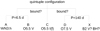 |
Fig. 3 Most likely configuration of AB 6 (see Sect. 6.3). |
| In the text | |
|
Fig. 4 Derived RVs for the components of AB 6 (see legend). |
| In the text | |
|
Fig. 5 Left panel: SB2 orbital solution for the WR binary in AB 6 (WR: black curve; O: green curve) using the complete set of RV measurements of the He II λ4686 line for star A and the He Iλ4471 line for star B (see legend). Right panel: same as left panel, but using the N V λλ4604, 4620 doublet RVsfor star A. See text for details. |
| In the text | |
|
Fig. 6 Combined Phoebe + wind-eclipse light curve model calculated for three inclinations (i = 45°, 65°, and the best-fitting value 57°; see legend), compared to the OGLE light curve (unbinned and binned at Δ ϕ = 0.03). Formal errors in the unbinned light curve are comparable to the symbol sizes. |
| In the text | |
|
Fig. 7 Left panel: dynamical spectrum of the He IIλ4686 line in velocity space. The RV curves of stars A and B are shown. Right panel: same as left panel, but with the contributionof the WR star subtracted. The residual emission excess (traced with the blue curve) follows the expected behavior of a WWC cone. |
| In the text | |
|
Fig. 8 Disentangled spectra of stars A, B, C, and D, shifted to their relative contribution in the visual. With only nine observationsand given the four stellar components, the reproduced strengths of the Balmer lines and important He lines are poorly constrained and should not be considered as real. |
| In the text | |
|
Fig. 9 Upper panel: comparison between observed photometry and flux-calibrated IUE and FUSE spectra (blue squares and lines) with the best-fitting model SED of AB 6 (red dotted line), which is the sum of the reddened SEDs of stars A, B, C, and D (black solid, green dotted, pink dashed, and cyan dot-dashed lines). Lower panels: comparison between normalized FUSE, IUE, and UVES spectra at ϕ ≈ 0.1 and the best-fitting normalized spectrum of AB 6, comprising the weighted models of stars A, B, C, and D. Line styles are as in the upper panel. |
| In the text | |
|
Fig. 10 Phase-dependent fits for various phases and spectral lines (see axes labeling). Line styles are as in Fig. 9. |
| In the text | |
|
Fig. 11 HST spectra at ϕ ≈ 0 (pink line) and 0.5 (blue line) in velocity space relative to the blue component of the C IV doublet corrected for the systemic velocity V0 = 196 km s−1. |
| In the text | |
|
Fig. 12 As in Fig. 1, but including the new position of star A. Apart from the Eddington limit (dashed gray line), we also plot mass-luminosity relations calculated for homogeneous stars with various hydrogen contents (see labeling). |
| In the text | |
|
Fig. 13 Best-fitting BPASS binary track for AB 6, calculated for Mi = 60 M⊙, qi = 0.7, and Pi = 16 d. The upper multi-colored track depicts the evolution of the WR primary until its core-collapse. The colors refer to surface hydrogen mass fractions of 0.45 < XH < 0.7 (blue), 0.2 < XH < 0.45 (red), 0.05 < XH < 0.2 (orange), and XH < 0.05 (green). The WC and RLOF phases are also marked. A track for a single 60 M⊙ star is shown for comparison (dashed gray line). The lower track depicts the evolution track of the O-type companion until the core collapse of the primary. |
| In the text | |
|
Fig. 14 As in Fig. 13, but depicting the best-fitting homogeneous evolution track calculated for a single Mi = 40 M⊙ star. The nonhomogeneous equivalent is shown for comparison (dashed line). |
| In the text | |
|
Fig. 15 Preliminary SB1 orbital solution derived for star D. |
| In the text | |
|
Fig. 16 Two UVES observations (MJD = 57944.4 58025.2 − 57944.4) that correspond to the maximum RV of star D. The left panel shows the N IV λ4060 line that belongs to star C, and the right panel shows the Si IVλ4089 line that belongs to star D. No antiphase motion can be seen in the spectrum of star C. |
| In the text | |
Current usage metrics show cumulative count of Article Views (full-text article views including HTML views, PDF and ePub downloads, according to the available data) and Abstracts Views on Vision4Press platform.
Data correspond to usage on the plateform after 2015. The current usage metrics is available 48-96 hours after online publication and is updated daily on week days.
Initial download of the metrics may take a while.