| Issue |
A&A
Volume 616, August 2018
|
|
|---|---|---|
| Article Number | A129 | |
| Number of page(s) | 9 | |
| Section | Interstellar and circumstellar matter | |
| DOI | https://doi.org/10.1051/0004-6361/201731768 | |
| Published online | 04 September 2018 | |
The December 2015 re-brightening of V404 Cygni
Variable absorption from the accretion disc outflow
1
Finnish Centre for Astronomy with ESO (FINCA), University of Turku, Väisäläntie 20, 21500 Piikkiö, Finland
e-mail This email address is being protected from spambots. You need JavaScript enabled to view it.
2
University of Oxford, Department of Physics, Astrophysics, Denys Wilkinson Building, Keble Road, Oxford OX1 3RH, UK
3
European Space Astronomy Centre (ESA/ESAC), Science Operations Department, 28691 Villanueva de la Cañada, Madrid, Spain
4
ESA/ESTEC, Keplerlaan 1, 2201 AZ Noordwijk, The Netherlands
Received:
14
August
2017
Accepted:
2
March
2018
Abstract
In December 2015 the black hole binary V404 Cyg underwent a secondary outburst after the main June 2015 event. We monitored this re-brightening with the INTEGRAL and Swift satellites, and in this paper we report the results of the time-resolved spectral analysis of these data. The December outburst shared several characteristics with the June event. The well-sampled INTEGRAL light curve shows up to ten Crab flares, which are separated by relatively weak non-flaring emission phases when compared to the June outburst. The spectra are nicely described by absorbed Comptonization models, with hard photon indices, Γ ≲ 2, and significant detections of a high-energy cut-off only during the bright flares. This is in contrast to the June outburst, where the Comptonization models gave electron temperatures mostly in the 30–50 keV range, while some spectra were soft (Γ ~ 2.5) without signs of any spectral cut-off. Similarly to the June outburst, we see clear signs of a variable local absorber in the soft energy band covered by Swift/XRT and INTEGRAL/JEM-X, which causes rapid spectral variations observed during the flares. During one flare, both Swift and INTEGRAL captured V404 Cyg in a state where the absorber was nearly Compton thick, N H ≈ 1024 cm−2, and the broad-band spectrum was similar to obscured AGN spectra, as seen during the X-ray plateaus in the June outburst. We conclude that the spectral behaviour of V404 Cyg during the December outburst was analogous with the first few days of the June outburst, both having hard X-ray flares that were intermittently influenced by obscuration due to nearly Compton-thick outflows launched from the accretion disc.
Key words: accretion, accretion disks / black hole physics / X-rays: binaries / X-rays: individuals: V404 Cyg
© ESO 2018
1. Introduction
Most black hole low-mass X-ray binaries show transient behaviour where they alternate between quiescence and outburst phases (for recent reviews, see Done et al. 2007; Belloni & Motta 2016). Occasionally weaker secondary outbursts (re-brightenings or re-flares) can follow the initial outbursts by a few weeks to a few months (e.g. Chen et al. 1993, 1997; Bailyn & Orosz 1995). Analogous secondary outbursts are also seen in systems where the compact object is a white dwarf (e.g. Kuulkers et al. 1996) or a neutron star (e.g. Lewis et al. 2010; Patruno et al. 2016), suggesting that they originate from some type of accretion disc instability or that they are due to an increase in the mass released from the companion star, induced by X-ray heating of its outer layers during the primary outburst (e.g. Tanaka & Lewin 1995; Lasota 2001). In 2015 the dynamically confirmed black hole binary V404 Cyg had two bright outbursts: a very bright one in June and a weaker secondary outburst in December. In this paper we concentrate on the X-ray spectral properties observed during the second event.
Similarly to the 1989 X-ray outburst (Tanaka 1989; in ’t Zand et al. 1992; Oosterbroek et al. 1996; Życki et al. 1999), during the June 2015 outburst V404 Cyg showed spectacular flaring activity not only in the X-rays (e.g. Rodriguez et al. 2015; Roques et al. 2015; Jenke et al. 2016), but also in the radio (Tetarenko et al. 2017), optical (Gandhi et al. 2016; Kimura et al. 2016), and in the γ rays (Loh et al. 2016; Piano et al. 2017). X-ray spectral analysis has revealed that the flaring was not solely due to mass accretion rate enhancements, but was also strongly influenced by a highly variable local absorber (Walton et al. 2017; Sánchez-Fernández et al. 2017; Motta et al. 2017a). Occasionally, the hydrogen column density exceeded N H ≈ 1.5 × 1024 cm−2, i.e. the absorber was Compton-thick (the optical depth through the absorber was above unity for Thomson scattering), thus reducing the emission levels throughout the electromagnetic spectrum (Motta et al. 2017a,b; Sánchez-Fernández et al. 2017). Our interpretation is that the absorption/obscuration was due to a dense and inhomogeneous outflow that was launched from the inner accretion disc, and that the observed flux variability was generated when thick clouds partially obscured the inner parts of the accretion disc, or when the absorber occasionally became Compton-thin, thus revealing the primary X-ray source. Additional and more direct evidence of winds/outflows has been found in high-resolution data taken in both the X-ray and optical bands. In Chandra grating observations (King et al. 2015) found P Cygni profiles that were indicative of outflow velocities of about a few thousand kilometers per second. Optical spectroscopy also revealed P Cygni profiles associated with a few emission lines during the flaring, and the subsequent nebular line emission suggested that significant mass loss had occurred during the outburst (Muñoz-Darias et al. 2016).
On 23 December 2015 the Swift/BAT telescope detected a re-brightening of V404 Cyg (Barthelmy et al. 2015). Subsequent X-ray, optical, and radio observations confirmed the onset of a new outburst (Muñoz-Darias et al. 2017) only four months after the end of the primary outburst, which started in June 2015 and reached the X-ray quiescence level early in August 2015 (Sivakoff et al. 2015; Plotkin et al. 2017). V404 Cyg was already active at least from 21 December 2015; INTEGRAL serendipitously detected it prior to the BAT trigger (see Malyshev et al. 2015 and Fig. 1). In the December outburst optical observations showed signs of winds similar to those during the June outburst, with outflow velocities of about ~ 2500 km s−1 (Muñoz-Darias et al. 2017). Both outbursts also showed up to two magnitude optical variability on one-hour timescales (Kimura et al. 2016, 2017), which were correlated with the X-ray flares. Furthermore, the radio activity was almost as intense as in June (Muñoz-Darias et al. 2017), suggesting that mass outflows through jets occurred in both outbursts. In this paper, we study the Swift and INTEGRAL X-ray spectra of V404 Cyg in order to establish whether the Compton-thick absorbers that were detected in June also play a role in the December outburst.
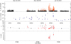 |
Fig. 1. Light curve and spectral parameter evolution of V404 Cyg during the December 2015 outburst. Top panel: 20–65 keV INTEGRAL/ISGRI light curve, scaled to Crab units. Red symbols are used for the flares. Second panel: 2–10 keV fluxes (in Crab units) from the individual Swift/XRT snapshots. Blue circles indicate data used to extract the non-flaring spectra. Third panel: photon index; the black symbols indicate the spectra accumulated by averaging the Swift and INTEGRAL non-flaring emission. Bottom panel: electron temperatures from the NTHCOMP model fits. |
2. INTEGRAL and Swift observations of V404 Cyg during the December 2015 outburst
The first INTEGRAL detection of V404 Cyg during the December re-brightening occurred in spacecraft revolution 1624, between 21 and 23 December 2015 (MJD 57377–57379). After the BAT detection on 23 December, we triggered target of opportunity INTEGRAL observations of V404 Cyg that lasted four consecutive revolutions (1626–1629), performed between 25 December 2015 and 5 January 2016. Several Swift observations were also triggered, and we analyse here the data that overlap with the INTEGRAL monitoring campaign. We indicate the observations and time intervals in Table 1. During the last INTEGRAL orbit the outburst was seen to fade by Swift, and soon after even the Swift monitoring had to be stopped due to Sun constraints on 20 January 2016. The outburst lasted some time beyond the Swift monitoring, as the AMI-LA radio light curve showed significant flaring activity up to 22 January 2016 (Muñoz-Darias et al. 2017).
Log of observations used in this work.
2.1. INTEGRAL
We make use of the public INTEGRAL IBIS/ISGRI light curves of V404 Cyg provided by the ISDC (Kuulkers & Ferrigno 2016). These light curves have a 64 s time resolution, which is appropriate to separate the X-ray flares from the non-flaring emission. The observed count rate histograms were converted to Crab units with the observed Crab ISGRI rate of 147 cps in the 25–60 keV band. Based on a close inspection of our dataset, we identified the flares in the ISGRI light curves as follows. We first estimated the non-flaring emission level as the mean ISGRI count rate during revolution 1624. To identify a flare we required at least four time bins (i.e. 256 s) to have a count rate 4.5 σ above the nonflaring emission level, but during a flare allowed two consecutive points to have a count rate value below the count rate threshold crossed at the onset of each flare before defining that the flare has ended. We then used the obtained time intervals to extract JEM-X and ISGRI spectra.
Since the non-flaring emission is rather faint we integrated over the non-flaring intervals to extract a spectrum in between flares. We refer to these data as non-flare emission (NFE). For the first three INTEGRAL orbits (NFEs 1, 3, and 4) we used the whole INTEGRAL orbit. However, for NFE5 we used only the first half of orbit 1628 where flares were seen, while for NFE6 we used the second half of orbit 1628 and the whole orbit of 1629 where no flares were seen (see Fig. 1). During the flares we performed time-resolved spectroscopy any time the number of counts in the flare exceeded a limit of 2 × 10⁵ in order to allow a good signal-to-noise ratio. If during a flare the total number of counts was lower than the above threshold, we integrated a single averaged spectrum of the flare. Conversely, whenever the INTEGRAL light curve had gaps (due to space craft slews or perigee passages) we deemed that a seemingly continuous flare had ended and started integrating the next flare (see Fig. 3).
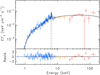 |
Fig. 2. Broad-band Swift/XRT (blue), INTEGRAL JEM-X (orange), and ISGRI (red) spectrum of V404 Cyg of the non-flare emission during MJD 57385–57387 (NFE4). The spectrum is nicely described by the partially covered Comptonization model, together with a significant, narrow iron line at 6.4 keV. The residuals are in units of sigma (delchi command in XSPEC). |
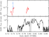 |
Fig. 3. Swift/XRT (top) and INTEGRAL/ISGRI (bottom) light curves of a flare during MJD 57388.72–57388.87 (Obs. ID 00031403134 from 1 January 2016). The XRT PC mode data is shown in red and the WT data in blue. Spectral changes during the first XRT snapshot are shown in Fig. 4 and the broad-band spectrum with INTEGRAL and the second Swift snapshot is shown in Fig. 5. The ISGRI-only flare extraction (FX) times tabulated in Table 3 are denoted with horizontal lines. |
In this manner we extracted 52 ISGRI and JEM-X flare spectra, and 5 non-flaring spectra. The IBIS/ISGRI and JEMX data reduction was performed using the Off-line Scientific Analysis software (OSA; Courvoisier et al. 2003) v10.2, using the latest calibration files. The data were processed following standard reduction procedures. We used good time interval (GTI) files generated from the flare start/end times calculated as described above to extract the flare spectra. We also used GTI files to avoid the flaring intervals in the extraction of the non-flaring spectra, which we also ignored 300 s before and after each flare to avoid potential flare contamination of the non-flaring intervals. For the flare spectra we binned the IBIS/ISGRI response matrix in the energy range 20–500 keV using 28 channels of variable logarithmic widths as in Sánchez-Fernández et al. (2017), while for the NFE spectra we used the ISGRI standard 13 channel binning. We restricted the spectral fits to the 20–200 keV energy range; above 200 keV there is an additional spectral component (Jourdain et al. 2017) and the ISGRI data are background dominated. In our flare fits we ignored the energy bin around 50 keV since this data point was systematically below the rest of the spectral bins, and as in Sánchez-Fernández et al. (2017) we added 3% systematic errors to the spectral bins. The JEMX response matrix in the energy range 3–35 keV was binned using the standard eight-channel energy bins defined in the OSA software for both flaring and non-flaring spectra. In our fits we ignored the first JEM-X energy bin and the noisy channels above 20 keV.
2.2. Swift/XRT
We extracted the Swift/XRT spectral data and light curves with the online Leicester XRT product generator (Evans et al. 2009). To generate the light curve in Crab units, we first converted the Swift/XRT count rates to fluxes using WebPIMMS (assuming Γ = 1.7 and NH = 0.83 × 1022 cm−2). This gave a conversion factor of 1 cps = 5.5 × 10⁻¹¹ erg cm−2 s−1 where the input was 0.3–10 keV band and output was in the 2–10 keV band. The conversion to Crab units was then done assuming a Crab flux of 2.4 × 10⁻⁸ erg cm−2 s−1.
In most of the observations the count rate was below 1 cps, and thus the data were taken in the photon counting (PC) mode. In general, observations showing non-flaring emission did not yield many detected photons in Swift, and we therefore had to average the non-flare XRT spectra to increase the signal-to-noise ratio, as indicated in Fig. 1 and Table 1. We note that we did not use the XRT data that were taken in between the INTEGRAL orbits. At the times when XRT data were taken during a major flare, some snapshots of a few hundred seconds were sufficient to determine the source spectral shape. In two cases, intrasnapshot variability was also detected (as highlighted below). In these cases we split the data further either based on the XRT count rate or on the observing mode because in the flare peaks XRT automatically switches to windowed timing (WT) mode. All the extracted spectra were binned to have a minimum of 20 counts per channel using the GRPPHA tool.
2.3. Spectral fits
We used XSPEC v12.8.2 to fit the extracted X-ray spectra. The best fitting parameters were obtained by minimizing the χ 2 statistics, and the errors provided below are quoted at the 1-σ confidence level (Δχ2 = 1 for one parameter of interest). We initially fitted the data from the three instruments using freely varying normalization constants, but later found that they were consistent with each other. Therefore, in the spectral fits discussed below these instrument cross-calibration constants are assumed to be unity.
Following our previous analysis of the June 2015 outburst (Sánchez-Fernández et al. 2017), we used the Comptonization model NTHCOMP (Zdziarski et al. 1996; Życki et al. 1999) to fit the spectral data. The spectral parameters are the power-law index Γ and the electron temperature Te, with the seed photon temperature fixed to 0.1 keV given that there were no indications of a low-energy cut-off in the XRT data. To account for the inhomogeneous local absorption that was present in the June outburst (Motta et al. 2017a), we multiply NTHCOMP with a partial covering model TBNEW_PCF and with a second, fully covering column fixed to the interstellar value of NH,ISM = 0.83 × 1022 cm−2 or higher if required by the data using TBNEW (obtained from optical reddening of AV = 4.0; Hynes et al. 2009 and assuming AV/NH(1021cm−2) = 0.48; Valencic & Smith 2015). We tested partial covering models on the INTEGRAL data, but found that the model parameters could not be constrained without simultaneous Swift/XRT data covering the lower energies. For this reason in the INTEGRAL-only fits we fixed the absorption column to the interstellar value. Similarly, when modelling only the Swift/XRT data, we used the simpler POWERLAW model since the high-energy cut-off was not visible in the XRT energy band (i.e. below 10 keV).
After fitting the data with these models we used the method described in Sánchez-Fernández et al. (2017) to determine whether a cut-off, an iron line, or an additional fully or partially covered absorption component was statistically required by the data. We first approximated the Bayesian information criterion (BIC) as BIC = χ2 + k ln(n), where k is the number of parameters in the model, and n is the number of channels in the spectral fits. Here a lower BIC implies either fewer explanatory variables, a better fit, or both. A model with more free parameters was selected if ΔBIC > 6, i.e. if the strength of the evidence against the model with the higher BIC was strong (Kass 1995).
In addition to the partially covered direct Comptonization model described above, we also fitted the mytorus model (Murphy & Yaqoob 2009; Yaqoob 2012) to one joint Swift/XRT– INTEGRAL/JEM-X–IBIS-ISGRI spectrum where high column densities were detected (JF2d). This spectral model has been developed to describe obscured AGN where a toroidal absorber reprocesses the central emission in the Compton-thick regime. The model can be adjusted to emulate a toroidal structure, either uniform or patchy, with a half-opening angle of 60° and consequently a covering fraction of 0.5. We successfully employed this model to describe a plateau spectrum during the June 2015 outburst of V404 Cyg (Motta et al. 2017b). The model used in the present work consists of a thermal Comptonization component (the COMPTT XSPEC model), which describes the intrinsic source spectrum, and two additional components (the MYTORUS zeroth-order continuum component and the MYTORUS scattered component). The model expression used in XSPEC is the following:
Here the optical depths τ and the model normalizations Nctt of the two Comptonization components COMPTT1 and COMPTT2 are linked to one another, the electron temperature is fixed to Te = 50 keV, and the seed photon temperature is fixed to T0 = 0.1 keV. The Te was found by fitting the INTEGRAL/ISGRI spectrum alone above 20 keV using only the zeroth-order continuum component (see Motta et al. 2017b) under the assumption that this component dominates the high energies (a reasonable assumption given the high local column density). Both of the MYTORUS components had inclinations fixed to 67 deg (Khargharia et al. 2010); the optical depth of the MYTORUS_SCATTERED was linked to the COMPTT component.
The first Comptonization component describes the intrinsic spectrum of the source, which does not interact at all with the toroidal absorber. The zeroth-order continuum is formed by the photons that are transmitted through the absorbing torus. The scattered continuum is, instead, the collection of all escaping photons that have been scattered in the medium at least once. This component, in principle, should include both the scattered continuum and the iron line complex. However, after a series of tests we found that the data we consider here do not allow us to determine whether a patchy reprocessor (requiring two scattered components, with inclination angles fixed at 0 and 90°, respectively) is statistically favoured with respect to a uniform reprocessor. Neither of the fits was significantly improved if we included the iron lines to the model. For these reasons the set-up of our model involves no lines, only one single scattered component and an inclination angle fixed to the source orbital inclination, which implies that the toroidal reprocessor is assumed to be uniform rather than patchy. In the fitting we changed the abundances to the values given by Anders & Grevesse (1989) from the default (Verner et al. 1996) values in order to match the abundances used in the MYTORUS tables, and we allowed the ISM column density parameter to vary freely.
3. Results
The INTEGRAL/ISGRI light curve of the December–January outburst is shown in the top panel of Fig. 1. The X-ray flaring characteristic of V404 Cyg outbursts is clearly visible from MJD 57385 onwards. The bottom panels of Fig. 1 also show the 2–10 keV fluxes of the individual Swift/XRT snapshots (in Crab units), as well as the time evolution of the NTHCOMP model parameters, after separating the flares and the non-flaring emission (see also Tables 2 and 3).
Best fitting parameters used to fit the non-flare emission and joint Swift and INTEGRAL flare data with the TBNEW × TBNEW_PCF × (NTHCOMP + GAUSS) MODEL.
Best fitting parameters used to fit the ISGRI flare data with the TBNEW × NTHCOMP model.
An example of a non-flare emission (NFE4) is shown in Fig. 2. This non-flare spectrum is the only one where a weak and narrow iron K-α line is seen, with an equivalent width of  . It is also the only spectrum where a good fit requires both a partially covering column and a fully covering column significantly above the interstellar value. This spectrum is also the softest of all the non-flare groups, with Γ ≈ 1.9 versus Γ ≈ 1.6, even though all the NFE spectra have approximately the same emitted flux until the flaring ceased and V404 Cyg became undetectable by INTEGRAL in the NFE6 group.
During the observing campaign two flares were captured jointly with Swift and INTEGRAL (denoted as JF1 and JF2 in Tables 1 and 2). A zoom-in of the second joint flare is shown in Fig. 3. The top panel shows the Swift/XRT light curve (Obs. ID 00031403134), with the PC mode data in red and the WT mode data of a flare peak in blue. In the bottom panel a simultaneous INTEGRAL/ISGRI light curve is also shown. Unfortunately, during the strongest XRT flare INTEGRAL slewed to the next pointing of its dither pattern, thus missing the action.
The spectral variations during the first Swift snapshot of this flare are shown in Fig. 4. The first PC mode time interval is shown in green, the WT mode time interval of the flare in orange, and the post flare PC mode interval in purple. Significant spectral changes are observed in this flare (see also Table 2). The best fitting spectral parameters show that at the beginning of the observation (JF2a) the 2–10 keV flux is already enhanced by a factor of two with respect to the non-flaring emission, and that a thick column of NH, pcf = [40 ± 7] × 1022 cm−2 that almost completely covers the source is required. The subsequent flare, where the sixfold increase in flux caused XRT to automatically switch from PC to WT mode, was instead best fit with only a modest, less covered absorber (JF2bm1) or, alternatively, without any partially covering column but with a significantly harder intrinsic spectrum (JF2bm2).Neither of these models can be statistically rejected given the relatively noisy XRT data, and without complementary INTEGRAL data to constrain the spectral slope. However, we note that no ISGRI spectra have photon indices below Γ ≲ 1.4 (see Tables 2 and 3); therefore, we favour the former best fit. After the flare the flux drops to a level higher than that seen prior to the flare, and is accompanied by an increase in the partially covering column (JF2c).
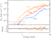 |
Fig. 4. Rapid spectral changes seen during a Swift snapshot taken on 1 January 2016 (OBS ID: 00031403134). The green spectrum was extracted during the first 590 s of the observation (JF2a), the orange spectrum is the WT mode segment covering the 120 s duration flare (JF2b), and the purple spectrum was taken during a 480 s segment posterior to the flare (JF2c). The variability can be nicely described by a rapid uncovering of the intrinsic emission. Similar variability was also seen in the June outburst (see Motta et al. 2017a, Fig. 3). |
The second Swift/XRT snapshot (JF2d) was taken between two strong ~2 Crab flares seen in the ISGRI data. We extracted a simultaneous INTEGRAL JEM-X–ISGRI spectra with this XRT snapshot, and the resulting broad-band spectrum is shown in Fig. 5. It can be described well with both the partially covered NTHCOMP model (see Table 2) and with the mytorus model, which is shown in the figure. Both models require the presence of a nearly Compton-thick absorber, with NH, pcf ~ 1024 cm−2. In the mytorus fit the high-energy emission is completely dominated by the so-called transmitted component (or zeroth-order component, see Murphy & Yaqoob 2009; Yaqoob 2012; Motta et al. 2017b, for details), which accounts for the emission passing through a thick toroidal reprocessor surrounding the source, with a column density of NH, pcf = [1.08 ± 0.06] × 1024 cm−2 (dashed line in Fig. 5). The direct Comptonization emission from the central X-ray source corresponding to the COMPTT1 component in the model description in Sect. 2.3 (dot-dashed line) is extremely faint overall, but it dominates the emission at lower energies. The scattered component (dotted line) is only marginally required to describe the data. The MYTORUS model allows us to fit the iron line complex (which constitutes part of the scattered emission) self-consistently with the scattered continuum through a dedicated line component. The normalizations of these two components can be linked to one another, so that the line flux is always consistent with the flux of the scattered continuum required by the data. However, we find a very low flux of the scattered continuum meaning that the line fluxes are also negligible, which together with the noisy XRT data implied that the line component was not statistically required in the fit. The best fitting optical depth of the Comptonized continuum is  (electron temperature was fixed to 50 keV). The observed flux in the 2–10 keV band is F2−10 ≈ 4.7 × 10⁻¹⁰ erg cm−2 s−1, but the intrinsic flux measured in the same band was higher by almost a factor of ten: F2−10 ≈ 4.2×10⁻⁹ erg cm−2 s−1. However, in the 20–200 keV band the observed flux was F20−200 ≈ 1.2 × 10⁻⁸ erg cm−2 s−1, which was only reduced by about 30% as the intrinsic flux in the same band is F20−200 ≈ 1.7 × 10⁻⁸ erg cm−2 s−1, consistent with the fact that the absorber in this flare was not Comptonthick.
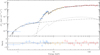 |
Fig. 5. Broad-band spectrum of V404 Cyg of a simultaneous Swift/XRT (blue), INTEGRAL JEM-X (orange), and ISGRI (red) observation during an X-ray flare JF2d (see Fig. 3). The spectrum can be described by a partially covered Comptonized continuum or, as shown here, by the mytorus model (Yaqoob 2012), which describes a thick toroidal reprocessor that scatters the emission of a point-like X-ray source located at the geometrical centre of the torus. The spectral component dominating at high energies is produced by the emission transmitted through a column of NH ≈ 1 × 1024 cm−2 (dashed line). The dot-dashed line marks the direct Comptonization emission from the source, while the dotted line represents the emission scattered within the toroidal reprocessor before reaching the observer. |
We identified 39 flares in the ISGRI light curve (see Table 3). However, flare 19 (F19) was too faint to perform a meaningful spectral analysis. Furthermore, in most flares the contemporaneous JEM-X data were very noisy, due to the high absorption columns and to the intrinsic X-ray spectra being so hard. Additionally, from the Swift/XRT data we knew that the absorption model had to be complex, but the JEM-X data alone were not sufficient to constrain the absorption parameters. For consistency we therefore decided to consider only the ISGRI spectra for the flares, and used the NTHCOMP model for these data following Sánchez-Fernández et al. (2017). The relations between the NTHCOMP model parameters are shown in Fig. 6, together with the results of the June outburst (in grey) presented in Sánchez-Fernández et al. (2017). The fits clearly show that during the December outburst V404 Cyg remained in the “hard flaring branch” (Fig. 6, panel a), where the spectra are described well by Γ ≈ 1.6 power law. Only in one bright flare do we see V404 Cyg with a softer Γ ≈ 2 power-law spectrum. We can also see a clear difference between the photon indices of the flare emission below and above F ≈ 5 × 10⁻⁹ erg cm−2 s−1. Above this threshold the spectra (consisting primarily of spectra of long flares) are clearly harder, with a weighted mean of Γ = 1.619 ± 0.004, while below it the spectra of mostly short flares have Γ = 1.75±0.02. In Fig. 6b we do not see a correlation between the electron temperatures with the emitted flux as in the June outburst. The relations between Te and shown in Fig. 6c cover the same parameter space as during the hard flares seen at the beginning of the June outburst, but again no clear correlation is seen.
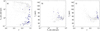 |
Fig. 6. Relations between the spectral parameters from the the NTHCOMP model fits during short and long INTEGRAL flares. The parameters from the June outburst are also shown (in grey). In the December outburst, V404 Cyg occupies mostly the “hard flaring branch” (panel a). In the Fx–Te diagram (panel b) we do not see the same anti-correlation as in June. Panel c: Γ−Te diagram. The fluxes are given in units of 10−8 erg cm−2 s−1. |
4. Discussion
All but one of the bright flares during the December 2015 outburst of V404 Cyg showed a hard spectrum, with Γ ≈ 1.6, similarly to what is seen in the spectra obtained during the first few days (i.e. the first INTEGRAL orbit) of the June outburst (Sánchez-Fernández et al. 2017). As in the June outburst, there is again no need to include thermal disc models in any of the spectra in the soft X-ray band, indicating that the thin disc is likely always truncated and the inner accretion flow consists of some sort of geometrically thick flow. The rapid flux and spectral variations seen during the flaring shown in Figs. 3 and 4 were consistent with being due to momentary uncovering of the central source from behind a local, non-uniform, and nearly Compton-thick neutral absorber. In addition, the spectrum taken between two INTEGRAL/ISGRI flux peaks shown in Fig. 5 strongly resemble the highly absorbed plateau spectra seen in June (Motta et al. 2017b; Sánchez-Fernández et al. 2017). A narrow emission feature at 6.4 keV consistent with the iron K-α line was detected in one case (NFE4) where thick absorbers were also present, similarly to what was observed in the June outburst. Hence, we conclude that the flares are again not solely due to accretion events, but their stochastic nature is also affected by local absorption/obscuration of the central source, exactly as in the previous X-ray outbursts from this system (Oosterbroek et al. 1996; Życki et al. 1999; Sánchez-Fernández et al. 2017; Motta et al. 2017a). In a sense, these similarities are not surprising given that the optical spectroscopic data in December–January (Muñoz-Darias et al. 2017) exhibited very similar signatures of outflows to those in June–July (Muñoz-Darias et al. 2016).
One clear difference between the December and June outbursts is seen during the periods between the flares. In June the non-flare emission (the 2–10 keV flux) was always above F2−10 ≳ 10−9 erg cm−2 s−1 (Motta et al. 2017a), while in the December outburst the non-flare emission was continuously at a relatively stable low-flux level at F2−10 ~ [2 − 10] × 10−11 erg cm−2 s−1. These differences are likely not due to stronger absorption/obscuration effects in the December outburst because the non-flare emission shows only modest local absorption columns. Rather, it is more likely that the average accretion rate was significantly lower in December (which gave a fainter out-of-flare emission) and that the flares resulted from accreting a few dense ‘waves’ or clumps where the accretion rate momentarily increased to near-Eddington levels1.
In the June outburst, column densities as high as NH ~ 3 × 1024 cm−2 were measured (Motta et al. 2017a), being particularly high during the plateau phases between bright flares (Motta et al. 2017b; Sánchez-Fernández et al. 2017). The analogous event in the December outburst (see Fig. 5) had roughly 3 times lower column density of NH ~ 1 × 1024 cm−2, which is close to the peak of the high-NH distribution obtained from the sample of ~1000 Swift/XRT spectra taken in June (see Fig. 5a in Motta et al. 2017a). Consequently, as such absorbers are only nearly Compton-thick, we did not witness a factor of ten decrease in the total emitted flux during December as we did in June. In Fig. 3 the flux drops in the high-energy ISGRI band were modest, less than a factor of two, consistent with the similar order of magnitude difference between the intrinsic mytorus flux and the observed one. It is therefore likely that the flux variability was not influenced by the absorption column changes to the same extent as in June. Nevertheless, the rapid, roughly oneminute timescale column variations seen in the flare shown in Fig. 4 are very similar to the spectral variations seen in June (see Fig. 3 in Motta et al. 2017a), and thus their origin is likely the same. As in the June outburst, our interpretation is that during the brightest flares the high accretion rate leads to radiatively driven outflows from the inner thick disc, but that the mass outflow rate was lower given that the December outburst was less intense.
The short flares seen in the December outburst in the flux ranges of F ~ [1 − 5] × 10−9 erg cm−2 s−1 were not commonly seen during the June outburst given that the emission was almost continuously above this range (Sánchez-Fernández et al. 2017). These short flares were significantly softer than the longer, bright flares that had Γ ≈ 1.6. It is interesting to note that in several other black hole binaries in the hard state, and in the AGN population as a whole, similar spectral softening is observed at comparable luminosity levels (Yang et al. 2015). These trends are attributed to changes in the amount of external seed photons from the truncated accretion disc that enter the Comptonized region (i.e. the hot flow or corona); at luminosities above L/LEdd ≳ 10−3 (F ≳ 5 × 10⁻⁹ erg cm−2 s−1 for V404 Cyg) the disc gradually becomes the dominant source of seed photons for Comptonization as the flux increases, which can explain the observed correlation between F and Γ seen in many sources (Zdziarski et al. 2003; Veledina et al. 2011; Yang et al. 2015; Kajava et al. 2016). There are not enough bright flares during the December outburst to see whether this trend holds, as it does in the June 2015 outburst where the brightest flares showed this correlation (Sánchez-Fernández et al. 2017).
The softening in the L/LEdd ≲ 10−3 regime (F ≲ 5 × 10⁻⁹ erg cm−2 s−1) instead could be caused by the disc being truncated so far away from the black hole that it can play no role in the Comptonization process, which means that the observed X-ray spectrum is produced solely via the synchrotron-self-Compton mechanism (Yang et al. 2015). In this regime the seed photons are generated within the hot-flow, and the F–Γ anti-correlation could be generated by the accretion flow becoming more and more optically thin as the mass accretion rate decreases (see e.g. Veledina et al. 2011). Perhaps this type of mechanism was operating in the short flares during the December outburst, giving rise to the softer flares in the F ~ [1 − 5] × 10−9 erg cm−2 s−1 flux range. It has also been speculated that the softening below L/LEdd ≲ 10−3 is related to the increased contribution of the jet emission to the X-ray band as the flux approaches quiescence (see e.g. Sobolewska et al. 2011, and references therein). However, the analysis of Plotkin et al. (2017) suggests that the jet does not contribute to the X-ray emission of V404 Cyg even near quiescence levels at L/LEdd ~ 10−6, and it is thus not likely that it plays a role at higher emission levels.
To conclude, the December 2015 re-brightening can be considered to be a full but failed hard-state outburst in which the source does not make a state transition to the soft state when approaching the Eddington limit (see e.g. Brocksopp et al. 2004; Koljonen et al. 2016; Kajava et al. 2016; Del Santo et al. 2016, for more recent studies of similar cases). The spectral variations in V404 Cyg are very similar to other black hole transients, notwithstanding the variable local absorption and the flaring events. However, during the December outburst V404 Cyg also did not enter the ultraluminous state (i.e. the very high state) even though accreting at near-Eddington levels, as was seen during the major soft flares in the main June 2015 outburst (Sánchez-Fernández et al. 2017) and also for example in the outbursts of GRO J1655–40 (Méndez et al. 1998; Motta et al. 2012). In other words, the disc is able to sustain a strong outflow whilst staying in the hard spectral state for at least up to ~20% of the Eddington flux. In the other flux extreme, we saw in the December outburst that the intrinsic NH variability occurs at practically all flux levels, also at orders of magnitude below the Eddington limit during the non-flaring emission at ~ 2 × 10⁻¹⁰ erg cm−2 s−1. This is interesting in terms of the launching mechanisms of the outflow. It is hard to imagine that at these lowest fluxes–more than 1000 times below the brightest flares–the outflow would only be radiatively driven, as suggested for the brightest flares during the June outburst Motta et al. 2017b,a; Sánchez-Fernández et al. 2017. Perhaps some other launching mechanism, such as a mildly relativistic outflowing corona driven by magnetic flares (Beloborodov 1999) or a magnetohydrodynamic wind (Fukumura et al. 2017), could be responsible for the NH-variability during these low-flux periods.
The 20–200 keV flux during the brightest INTEGRAL flare F24c reached about 20% of the Eddington limit.
Acknowledgments
We thank the anonymous referee whose comments helped to significantly improve the manuscript. JJEK acknowledges support from the Academy of Finland grant 295114 and the European Space Astronomy Centre (ESAC) for hospitality. SEM acknowledges support from the Violette and Samuel Glasstone Research Fellowship programme and from the UK Science and Technology Facilities Council (STFC). SEM and CSF acknowledge support from the ESAC Faculty. Based on observations with INTEGRAL, an ESA project with instruments and science data centre funded by ESA member states (especially the PI countries: Denmark, France, Germany, Italy, Switzerland, Spain), and Poland, and with the participation of Russia and the USA. We acknowledge the use of public data from the Swift data archive.
References
- Anders, E., & Grevesse, N. 1989, Geochim. Cosmochim. Acta, 53, 197 [Google Scholar]
- Bailyn, C. D., & Orosz, J. A. 1995, ApJ, 440, L73 [NASA ADS] [CrossRef] [Google Scholar]
- Barthelmy, S. D., Page, K. L., & Palmer, D. M. 2015, GRB Coordinates Network, 18716 [Google Scholar]
- Belloni, T. M., & Motta, S. E. 2016, Astrophys. Space Sci. Lib., 440, 61 [Google Scholar]
- Beloborodov, A. M. 1999, ApJ, 510, L123 [NASA ADS] [CrossRef] [Google Scholar]
- Brocksopp, C., Bandyopadhyay, R. M., & Fender, R. P. 2004, New Ast., 9, 249 [NASA ADS] [CrossRef] [Google Scholar]
- Chen, W., Livio, M., & Gehrels, N. 1993, ApJ, 408, L5 [NASA ADS] [CrossRef] [Google Scholar]
- Chen, W., Shrader, C. R., & Livio, M. 1997, ApJ, 491, 312 [NASA ADS] [CrossRef] [Google Scholar]
- Courvoisier, T. J.-L., Walter, R., Beckmann, V., et al. 2003, A&A, 411, L53 [NASA ADS] [CrossRef] [EDP Sciences] [Google Scholar]
- Del Santo, M., Belloni, T. M., Tomsick, J. A., et al. 2016, MNRAS, 456, 3585 [NASA ADS] [CrossRef] [Google Scholar]
- Done, C., Gierliński, M., & Kubota, A. 2007, A&ARv, 15, 1 [NASA ADS] [CrossRef] [EDP Sciences] [Google Scholar]
- Evans, P. A., Beardmore, A. P., Page, K. L., et al. 2009, MNRAS, 397, 1177 [NASA ADS] [CrossRef] [Google Scholar]
- Fukumura, K., Kazanas, D., Shrader, C., et al. 2017, Nature Astron., 1, 0062 [NASA ADS] [CrossRef] [Google Scholar]
- Gandhi, P., Littlefair, S. P., Hardy, L. K., et al. 2016, MNRAS, 459, 554 [NASA ADS] [CrossRef] [Google Scholar]
- Hynes, R. I., Bradley, C. K., Rupen, M., et al. 2009, MNRAS, 399, 2239 [NASA ADS] [CrossRef] [Google Scholar]
- in ’t Zand, J. J. M., Pan, H. C., Bleeker, J. A. M., et al. 1992, A&A, 266, 283 [NASA ADS] [Google Scholar]
- Jenke, P. A., Wilson-Hodge, C. A., Homan, J., et al. 2016, ApJ, 826, 37 [NASA ADS] [CrossRef] [Google Scholar]
- Jourdain, E., Roques, J.-P., & Rodi, J. 2017, ApJ, 834, 130 [NASA ADS] [CrossRef] [Google Scholar]
- Kajava, J. J. E., Veledina, A., Tsygankov, S., & Neustroev, V. 2016, A&A, 591, A66 [NASA ADS] [CrossRef] [EDP Sciences] [Google Scholar]
- Kass, R., Raftery, A. 1995, J. Am. Stat. Assoc., 90, 773 [Google Scholar]
- Khargharia, J., Froning, C. S., & Robinson, E. L. 2010, ApJ, 716, 1105 [NASA ADS] [CrossRef] [Google Scholar]
- Kimura, M., Isogai, K., Kato, T., et al. 2016, Nature, 529, 54 [NASA ADS] [CrossRef] [Google Scholar]
- Kimura, M., Kato, T., Isogai, K., et al. 2017, MNRAS, 471, 373 [NASA ADS] [CrossRef] [Google Scholar]
- King, A. L., Miller, J. M., Raymond, J., Reynolds, M. T., & Morningstar, W. 2015, ApJ, 813, L37 [NASA ADS] [CrossRef] [Google Scholar]
- Koljonen, K. I. I., Russell, D. M., Corral-Santana, J. M., et al. 2016, MNRAS, 460, 942 [NASA ADS] [CrossRef] [Google Scholar]
- Kuulkers, E., & Ferrigno, C. 2016, ATel, 8512 [Google Scholar]
- Kuulkers, E., Howell, S. B., & van Paradijs, J. 1996, ApJ, 462, L87 [NASA ADS] [CrossRef] [Google Scholar]
- Lasota, J.-P. 2001, New Astron. Rev., 45, 449 [NASA ADS] [CrossRef] [Google Scholar]
- Lewis, F., Russell, D. M., Jonker, P. G., et al. 2010, A&A, 517, A72 [NASA ADS] [CrossRef] [EDP Sciences] [Google Scholar]
- Loh, A., Corbel, S., Dubus, G., et al. 2016, MNRAS, 462, L111 [NASA ADS] [CrossRef] [Google Scholar]
- Malyshev, D., Savchenko, V., Ferrigno, C., Bozzo, E., & Kuulkers, E. 2015, ATel, 8458 [Google Scholar]
- Méndez, M., Belloni, T., & van der Klis, M. 1998, ApJ, 499, L187 [NASA ADS] [CrossRef] [Google Scholar]
- Motta, S., Homan, J., Muñoz Darias, T., et al. 2012, MNRAS, 427, 595 [NASA ADS] [CrossRef] [Google Scholar]
- Motta, S. E., Kajava, J. J. E., Sánchez-Fernández, C., et al. 2017a, MNRAS, 471, 1797 [NASA ADS] [CrossRef] [Google Scholar]
- Motta, S. E., Kajava, J. J. E., Sánchez-Fernández, C., Giustini, M., & Kuulkers, E. 2017b, MNRAS, 468, 981 [NASA ADS] [CrossRef] [Google Scholar]
- Muñoz-Darias, T., Casares, J., Mata Sánchez, D., et al. 2016, Nature, 534, 75 [NASA ADS] [CrossRef] [Google Scholar]
- Muñoz-Darias, T., Casares, J., Mata Sánchez D., et al. 2017, MNRAS, 465, L124 [NASA ADS] [CrossRef] [Google Scholar]
- Murphy, K. D., & Yaqoob, T. 2009, MNRAS, 397, 1549 [NASA ADS] [CrossRef] [Google Scholar]
- Oosterbroek, T., van der Klis, M., Vaughan, B., et al. 1996, A&A, 309, 781 [NASA ADS] [Google Scholar]
- Patruno, A., Maitra, D., Curran, P. A., et al. 2016, ApJ, 817, 100 [NASA ADS] [CrossRef] [Google Scholar]
- Piano, G., Munar-Adrover, P., Verrecchia, F., Tavani, M., & Trushkin, S. A. 2017, ApJ, 839, 84 [NASA ADS] [CrossRef] [Google Scholar]
- Plotkin, R. M., Miller-Jones, J. C. A., Gallo, E., et al. 2017, ApJ, 834, 104 [NASA ADS] [CrossRef] [Google Scholar]
- Rodriguez, J., Cadolle Bel, M., Alfonso-Garzón, J., et al. 2015, A&A, 581, L9 [NASA ADS] [CrossRef] [EDP Sciences] [Google Scholar]
- Roques, J.-P., Jourdain, E., Bazzano, A., et al. 2015, ApJ, 813, L22 [NASA ADS] [CrossRef] [Google Scholar]
- Sánchez-Fernández, C., Kajava, J. J. E., Motta, S. E., & Kuulkers, E. 2017, A&A, 602, A40 [NASA ADS] [CrossRef] [EDP Sciences] [Google Scholar]
- Sivakoff, G. R., Bahramian, A., Altamirano, D., et al. 2015, ATel, 7959 [Google Scholar]
- Sobolewska, M. A., Papadakis, I. E., Done, C., & Malzac, J. 2011, MNRAS, 417, 280 [NASA ADS] [CrossRef] [Google Scholar]
- Tanaka, Y. 1989, ESA SP, 296 [Google Scholar]
- Tanaka, Y., & Lewin, W. H. G. 1995, X-ray Binaries, 126 [Google Scholar]
- Tetarenko, A. J., Sivakoff, G. R., Miller-Jones, J. C. A., et al. 2017, MNRAS, 469, 3141 [NASA ADS] [CrossRef] [Google Scholar]
- Valencic, L. A., & Smith, R. K. 2015, ApJ, 809, 66 [NASA ADS] [CrossRef] [Google Scholar]
- Veledina, A., Vurm, I., & Poutanen, J. 2011, MNRAS, 414, 3330 [NASA ADS] [CrossRef] [Google Scholar]
- Verner, D. A., Ferland, G. J., Korista, K. T., & Yakovlev, D. G. 1996, ApJ, 465, 487 [NASA ADS] [CrossRef] [Google Scholar]
- Walton, D. J., Mooley, K., King, A. L., et al. 2017, ApJ, 839, 110 [NASA ADS] [CrossRef] [Google Scholar]
- Yang, Q.-X., Xie, F.-G., Yuan, F., et al. 2015, MNRAS, 447, 1692 [NASA ADS] [CrossRef] [Google Scholar]
- Yaqoob, T. 2012, MNRAS, 423, 3360 [NASA ADS] [CrossRef] [Google Scholar]
- Zdziarski, A. A., Johnson, W. N., & Magdziarz, P. 1996, MNRAS, 283, 193 [NASA ADS] [CrossRef] [Google Scholar]
- Zdziarski, A. A., Lubiński, P., Gilfanov, M., & Revnivtsev, M. 2003, MNRAS, 342, 355 [NASA ADS] [CrossRef] [Google Scholar]
- Życki, P. T., Done, C., & Smith, D. A. 1999, MNRAS, 309, 561 [NASA ADS] [CrossRef] [Google Scholar]
All Tables
Best fitting parameters used to fit the non-flare emission and joint Swift and INTEGRAL flare data with the TBNEW × TBNEW_PCF × (NTHCOMP + GAUSS) MODEL.
Best fitting parameters used to fit the ISGRI flare data with the TBNEW × NTHCOMP model.
All Figures
|
Fig. 1. Light curve and spectral parameter evolution of V404 Cyg during the December 2015 outburst. Top panel: 20–65 keV INTEGRAL/ISGRI light curve, scaled to Crab units. Red symbols are used for the flares. Second panel: 2–10 keV fluxes (in Crab units) from the individual Swift/XRT snapshots. Blue circles indicate data used to extract the non-flaring spectra. Third panel: photon index; the black symbols indicate the spectra accumulated by averaging the Swift and INTEGRAL non-flaring emission. Bottom panel: electron temperatures from the NTHCOMP model fits. |
| In the text | |
|
Fig. 2. Broad-band Swift/XRT (blue), INTEGRAL JEM-X (orange), and ISGRI (red) spectrum of V404 Cyg of the non-flare emission during MJD 57385–57387 (NFE4). The spectrum is nicely described by the partially covered Comptonization model, together with a significant, narrow iron line at 6.4 keV. The residuals are in units of sigma (delchi command in XSPEC). |
| In the text | |
|
Fig. 3. Swift/XRT (top) and INTEGRAL/ISGRI (bottom) light curves of a flare during MJD 57388.72–57388.87 (Obs. ID 00031403134 from 1 January 2016). The XRT PC mode data is shown in red and the WT data in blue. Spectral changes during the first XRT snapshot are shown in Fig. 4 and the broad-band spectrum with INTEGRAL and the second Swift snapshot is shown in Fig. 5. The ISGRI-only flare extraction (FX) times tabulated in Table 3 are denoted with horizontal lines. |
| In the text | |
|
Fig. 4. Rapid spectral changes seen during a Swift snapshot taken on 1 January 2016 (OBS ID: 00031403134). The green spectrum was extracted during the first 590 s of the observation (JF2a), the orange spectrum is the WT mode segment covering the 120 s duration flare (JF2b), and the purple spectrum was taken during a 480 s segment posterior to the flare (JF2c). The variability can be nicely described by a rapid uncovering of the intrinsic emission. Similar variability was also seen in the June outburst (see Motta et al. 2017a, Fig. 3). |
| In the text | |
|
Fig. 5. Broad-band spectrum of V404 Cyg of a simultaneous Swift/XRT (blue), INTEGRAL JEM-X (orange), and ISGRI (red) observation during an X-ray flare JF2d (see Fig. 3). The spectrum can be described by a partially covered Comptonized continuum or, as shown here, by the mytorus model (Yaqoob 2012), which describes a thick toroidal reprocessor that scatters the emission of a point-like X-ray source located at the geometrical centre of the torus. The spectral component dominating at high energies is produced by the emission transmitted through a column of NH ≈ 1 × 1024 cm−2 (dashed line). The dot-dashed line marks the direct Comptonization emission from the source, while the dotted line represents the emission scattered within the toroidal reprocessor before reaching the observer. |
| In the text | |
|
Fig. 6. Relations between the spectral parameters from the the NTHCOMP model fits during short and long INTEGRAL flares. The parameters from the June outburst are also shown (in grey). In the December outburst, V404 Cyg occupies mostly the “hard flaring branch” (panel a). In the Fx–Te diagram (panel b) we do not see the same anti-correlation as in June. Panel c: Γ−Te diagram. The fluxes are given in units of 10−8 erg cm−2 s−1. |
| In the text | |
Current usage metrics show cumulative count of Article Views (full-text article views including HTML views, PDF and ePub downloads, according to the available data) and Abstracts Views on Vision4Press platform.
Data correspond to usage on the plateform after 2015. The current usage metrics is available 48-96 hours after online publication and is updated daily on week days.
Initial download of the metrics may take a while.