| Issue |
A&A
Volume 615, July 2018
|
|
|---|---|---|
| Article Number | A99 | |
| Number of page(s) | 9 | |
| Section | Galactic structure, stellar clusters and populations | |
| DOI | https://doi.org/10.1051/0004-6361/201832903 | |
| Published online | 20 July 2018 | |
The vertical force in the solar neighbourhood using red clump stars in TGAS and RAVE
Constraints on the local dark matter density
Kapteyn Astronomical Institute, University of Groningen,
Landleven 12,
9747 AD
Groningen,
The Netherlands
e-mail: This email address is being protected from spambots. You need JavaScript enabled to view it.
Received:
26
February
2018
Accepted:
19
March
2018
Abstract
Aims. We investigate the kinematics of red clump (RC) stars in the solar neighbourhood by combining data from Tycho-Gaia Astrometric Solution (TGAS) and Radial Velocity Experiment (RAVE) to constrain the local dark matter density.
Methods. After calibrating the absolute magnitude of RC stars, we characterized their velocity distribution over a radial distance range of 6−10 kpc and up to 1.5 kpc away from the Galactic plane. We then applied the axisymmetric Jeans equations on subsets representing the thin and thick disks to determine the (local) distribution of mass near the disk of our Galaxy.
Results. Our kinematic maps are well behaved, permitting a straightforward local determination of the vertical force, which we find to be Kzthin = − 2454 ± 619 (km s−1)2 kpc−1 and Kzthick = − 2141 ± 774 (km s−1)2 kpc−1 at 1.5 kpc away from the Galactic plane for the thin and thick disk samples and for thin and thick disk scale heights of 0.28 kpc and 1.12 kpc, respectively. These measurements can be translated into a local dark matter density ρDM ~ 0.018 ± 0.002 M⊙ pc−3. The systematic error on this estimate is much larger than the quoted statistical error, since even a 10% difference in the scale height of the thin disk leads to a 30% change in the value of ρDM and a nearly equally good fit to the data.
Key words: Galaxy: kinematics and dynamics / solar neighborhood / dark matter
© ESO 2018
1 Introduction
With the launch of the Gaia satellite a wealth of new data is becoming available on the motions and positions of stars in the Milky Way and its satellite galaxies (Gaia Collaboration 2016a,b). For example, its first data release (Gaia DR1) containing the Tycho-Gaia Astrometric Solution (TGAS) has provided parallaxes that are roughly a factor two more precise (and proper motions of similar quality) than those in the hipparcos catalogue (ESA 1997), but for a sample that is unbiased and nearly 20 times larger. Furthermore, and specifically for the hipparcos stars themselves, the improvement in the proper motions is more than a factor 10 (Lindegren et al. 2016). The power of these data increases even further when combined with spectroscopic surveys such as the Radial Velocity Experiment (RAVE; Kunder et al. 2017), the Apache Point Observatory Galactic Evolution Experiment (APOGEE; Majewski et al. 2017) and the Large Sky Area Multi-Object Fiber Spectroscopic Telescope (LAMOST; Cui et al. 2012), as this provides knowledge of the full phase-space distribution of stars near the Sun, as shown in, for example, Allende Prieto et al. (2016), Helmi et al. (2017), Liang et al. (2017), Monari et al. (2017), Yu & Liu (2018).
New kinematic maps of the solar neighbourhood can be used, for example, to obtain more precise estimates of the local dark matter density ρDM. Most modern measurements of ρDM using the vertical kinematics of stars seem to be consistent with a value just below ~0.01 M⊙ pc−3 when assuming a total baryonic surface mass density Σbaryon of 55 M⊙ pc−2 (Read 2014). McKee et al. (2015) argued for a value of 0.013 M⊙ ∕pc−3 for Σbaryon = 47.1 M⊙ pc−2, and Bienaymé et al. (2014) found ρDM = 0.0143 ± 0.0011 M⊙ pc−3 for Σbaryon = 44.4 ± 4.1 M⊙ pc−2 using red clump (RC) stars in RAVE DR4. Recently Sivertsson et al. (2018) determined a dark matter density of 0.012 M⊙ pc−3 using SDSS-SEGUE G-dwarf stars for Σbaryon = 46.85 M⊙ pc−2. These estimates are consistent with those inferred from studying the local equation of centrifugal equilibrium (Salucci et al. 2010) or from studies that model the mass of the Milky Way globally (e.g. Piffl et al. 2014).
Despite the apparent good agreement between the various values reported in the literature, local dark matter density estimates are affected by different systematic uncertainties (see e.g. Silverwood et al. 2016). These include of course, uncertainties on Σbaryon, which depend on the gas mass density, which typically has an error of 50%, and the local stellar densities although these are typically determined with 10% accuracy or better (e.g. Holmberg & Flynn 2000; Bovy 2017). Furthermore, the presence of multiple populations and assumptions made regarding their distributions (e.g. Moni Bidin et al. 2012; Büdenbender et al. 2015; Hessman 2015) or deviations from equilibrium, such as bending or breathing ofthe disk (Widrow et al. 2012; Williams et al. 2013), may also affect the conclusions reached. For example, Banik et al. (2017) showed that breathing modes alone may lead to systematic errors of order 25% in ρDM.
In this paper we use TGAS and RAVE data to derive an estimate of the local dark matter density and explore the impact of uncertainties in (some of) the characteristic parameters of the Galactic thin and thick disks. In Sect. 2 we present the data and selection criteria used in this work as well as the new kinematic maps of the solar neighbourhood. In Sect. 3 we present our local dark matter measurement and the impact of the disk parameters on the estimate. We conclude in Sect. 4.
2 Data
The dataset we use stems from the cross-match of TGAS and RAVE DR5. The TGAS dataset contains ~ 2 million starsthat are in common between the Gaia DR1 catalogue and the HIPPARCOS and Tycho-2 catalogues and provides accurate positions on the sky, mean proper motions and parallaxes. The RAVE survey is a magnitude-limited survey (9 < I < 12) of stars in the southern hemisphere (~450 000 stars), that for low Galactic latitudes (b < 25°) uses a colour criterion, J − Ks ≥ 0.5, which preferentially selects giant stars. RAVE provides radial velocities, astrophysical parameters, as well as a spectro-photometric parallaxes. The overlap between RAVE DR5 and TGAS contains ~ 250 000 stars with full phase space information. McMillan et al. (2018, PJM2018 hereafter) used the TGAS astrometric parallax measurements as priors to derive improved spectro-photometric parallaxes and astrophysical parameters. This is the dataset that we use here, after applying a few extra quality cuts. We keep only those stars that have SNR_K > 20, an ALGO_CONV parameter equal to either 0 or 4, eHRV < 8 km s−1, and flag_any = 0. This leaves us with a “reliable” sample containing 108 679 stars. The median distance of stars in this sample is of ~0.5 kpc, and their median relative distance error is ~13%.
2.1 Selecting a red clump stars’ sample
To gain more in distance accuracy we use RC stars, as they act as standard candles (e.g. Paczyński & Stanek 1998; Groenewegen 2008; Girardi 2016). We select RC stars on the basis of the surface gravity  and the extinction-corrected 2MASS bands Jcorr and KS,corr, where Jcorr = J − AJ and
 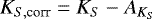 , and AJ = 0.282 AV and
  , where AV is taken from PJM2018. Finally we define our “RC sample” by:
 (1)
(1)
and which contains 26 653 stars. We calibrate the RC absolute Ks -band magnitude by considering a subsample of 3211 RC stars with a maximum relative parallax error of 10%. We find these stars to havea mean absolute Ks-band magnitude of  mag and a dispersion of0.064 mag, which we round-offto
  mag and a dispersion of 0.1 mag (which translates into a ~5% error in distance) in the remainder of this work. These values depend slightly on the maximum parallax error imposed for the calibration, and they are consistent with Hawkins et al. (2017), who find
  mag and a dispersion of 0.17 ± 0.02, and Ruiz-Dern et al. (2018) who find
  mag, both works mainly using TGAS parallaxes and APOGEE spectroscopy.
In the left panel of Fig. 1 we show the distribution of giant branch stars in our sample in the extinction-corrected  colour versus surface gravity
  space. Our selection of RC stars is given by the light blue box. In this region there will be some contamination of red giant branch (RGB) starssince RAVE does not provide asteroseismic information that can be used to discriminate between RC and RGB stars (e.g. Bedding et al. 2011; Chaplin & Miglio 2013). According to Girardi (2016) the typical contamination fraction is of order 30% of the log (g) box width in dex used to define the RC sample, thus resulting in a contamination estimate of 7.5% for our RC selection criteria. In the right panel of Fig. 1 we show a similar region of an extinction-corrected HR diagram using the PJM2018 improved parallaxes for the stars from the reliable sample. The mean and standard deviation of the adopted RC absolute KS -band magnitude are plotted as the horizontal solid and dashed lines, respectively.
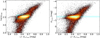 |
Fig. 1 Selection and calibration of RC stars. Left: distribution of giant stars in our sample in the extinction-corrected colour vs. surface gravity space. The blue lines enclose our RC sample. Right: extinction-corrected HR diagram of stars in our sample. The solid and dashed light blue lines indicate the adopted mean and standard deviation of the RC absolute KS -band magnitude, respectively. |
2.2 General properties of the RC sample
Now that we calibrated the mean absolute magnitude of RC stars and its spread, we proceed to compute distances to our stars. We define a default realization in which all RC stars are assumed to have  mag. The resulting spatial distribution of stars is shown in Fig. 2 and is computed in bins with widths 0.5 kpc in R and 0.1 kpc in z after setting R⊙ = 8.3 kpc (Schönrich 2012) and z⊙ = 0.014 kpc (Binney et al. 1997) for the position of the Sun with respect to the Galactic centre. This figure shows that our sample covers R ~ 6 − 10 kpc and |z| ≲ 1.5 kpc. Since the RAVE survey is more orientated to the southern and inner part of the Galaxy, there are more RC stars observed in these regions.
When converting the observables to Galactocentric cylindrical coordinates and velocities, we additionally use
 km s−1 (Schönrich et al. 2010) for the peculiar motion of the Sun with respect to the local standard of rest (LSR), and where U is radially inward, V in the direction of Galactic rotation, and W perpendicular to the Galactic plane and positive towards the north Galactic pole;
vc(R⊙) = 240 km s−1 (Piffl et al. 2014) for the circular velocity at R = R⊙.
Figures 3 and 4 show kinematic maps, i.e. mean velocities and their standard deviations, respectively, in the meriodional plane using the same default realization and bin widths as before. These figures show the well-known decrease of the average rotational velocity ⟨vϕ⟩ with height above the plane and the increase of the velocity dispersions with increasing |z|. We also see a variation (of order 5 km s−1 kpc−1) in ⟨vR⟩ with respect to R and some asymmetry in the vertical direction, as found in other works (e.g. Casetti-Dinescu et al. 2011; Siebert et al. 2011; Williams et al. 2013). On the other hand we do not find strong evidence for a bending or breathing mode in ⟨vz ⟩, at least up to 0.7 kpc (see also Carrillo et al. 2018).
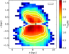 |
Fig. 2 Meridional plane RC star counts in bins of 0.5 kpc in R and 0.1 kpc in z (as indicated by the box in the upper right corner). The white contours indicate where the number of RC stars in the bins have dropped to 200, 100, and 50 from inner to outer contours respectively. The black symbol marks the position of the Sun. This figure is based on the default realization in which the absolute magnitudes of all RC stars are set to
|

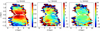 |
Fig. 3 Mean velocities of RC stars in the meridional plane based on the default realization in which the absolute magnitudes of all RC stars are set to |

3 Local dark matter density estimate
Now that we have constructed a good quality kinematic dataset, we proceed to estimate the local dark matter density in the steady-state axisymmetric limit. Although our kinematic maps reveal some deviations, these are of sufficiently small amplitude1 that we neglect them in our analysis. In this section, we first discuss the basic equations that relate the mass density to the kinematic moments, then describe how we measure these moments, and finally present our new determination and discuss the influence of the uncertainties on the main parameters of our mass model.
3.1 Surface mass density and the vertical Jeans equation
The (integrated) Poisson equation in cylindrical coordinates links the total surface mass density Σ (R, z) to the components of the gravitational force per unit mass in the radial, FR, and vertical direction, Kz, via
 (2)
(2)
where  .
.
Under the assumption of equilibrium, we can use the Jeans equations to relate the moments of the distribution function of a population, such as its density and velocity moments, to the gravitational potential in which it moves Φ (R, z). In this case,
![Mathematical equation: \begin{equation*}\begin{split} K_z &\equiv -\frac{\partial \mathrm{\Phi}}{\partial z} \\ &= - \frac{\langle v^2_{z} \rangle}{z} \left[\gamma_{\ast,z} + \gamma_{\langle v^2_{z} \rangle,z }\right] + \frac{\langle v_{R}v_{z}\rangle}{R} \left[1 - \gamma_{\ast,R} - \gamma_{\langle v_{R}v_{z} \rangle,R }\right] \end{split} \end{equation*}](/articles/aa/full_html/2018/07/aa32903-18/aa32903-18-eq17.png) (3)
(3)
and
![Mathematical equation: \begin{equation*}\begin{split} F_R &\equiv -\frac{\partial \mathrm{\Phi}}{\partial R} \\ &= - \frac{\langle v^2_{\phi} \rangle}{R} + \frac{\langle v^2_{R} \rangle}{R} \left[1-\gamma_{\ast,R} - \gamma_{\langle v^2_{R} \rangle,R }\right] - \frac{\langle v_{R}v_{z}\rangle}{z} \left[\gamma_{\ast,z} + \gamma_{\langle v_{R}v_{z} \rangle,z}\right]. \end{split} \end{equation*}](/articles/aa/full_html/2018/07/aa32903-18/aa32903-18-eq18.png) (4)
(4)
In these equations we have defined
![Mathematical equation: \begin{equation*} \gamma_{Q,x} \equiv - \frac{\partial\ln \left[Q(x)\right]}{\partial\ln \left[x\right]}, \nonumber \end{equation*}](/articles/aa/full_html/2018/07/aa32903-18/aa32903-18-eq19.png)
where γ*,x is the log-slope of the stellar density profile of the population with respect to coordinate x (=R or z), and otherwise γQ,x denotes the log-slope of the velocity moments. The steady-state assumption implies that ⟨vR ⟩ = ⟨vz⟩ = 0, and hence cov(vR, vz) = ⟨vRvz⟩, and  , and analogously for σ2(vz).
From Eqs. (3) and (4) and using the kinematic moments, we can derive the force field, which when inserted in Eq. (2), allows us to derive the total surface mass density. This includes the contributions of all baryonic components and a putative dark matter component, whose contribution we can establish with the data. We note, therefore, that not only accurate measurements of the velocity moments and their variation with R and z are needed, but also knowledge of the radial and vertical slopes of the density distribution, and the surface densities of the various baryonic components; i.e. interstellar medium (ISM) and stars. Since our dataset does not allow us to derive these quantities reliably, we have to make additional assumptions.
To reduce the complexity of the problem, one may note that the last term of Eq. (2) is approximately zero near R = R⊙ and z = 0, since the circular velocity curve  is approximately flat at the solar Galactocentric radius (e.g. Reid et al. 2014). Kuijken & Gilmore (1989) showed that in this case the term can be neglected up to a few kpc in z. Furthermore, Bovy & Tremaine (2012) showed that
  decreases as one moves away from the midplane for reasonable models of the Milky Way (although this has been challenged by Moni Bidin et al. 2015). Therefore dropping the term leads to an underestimate of the surface mass density Σ (R, z), which Bovy& Tremaine (2012) found in their models to be a few percent at z = 1.5 kpc up to roughly 15% at z = 4 kpc.
Our dataset does not extend to heights larger than 1.5 kpc, which implies that we can solve the integrated Poisson equation by only evaluating the vertical Jeans equation. We assume an exponential disk and that σ2(vR) and σ2(vz) follow an exponential profile in R with the same scale length as the density (e.g. van der Kruit & Searle 1982; Lewis & Freeman 1989). For the tilt angle, which relates to the last term in Eq. (3), we do not assume spherical alignment2 but that it is constant with R. We then combine Eqs. (2) and (3) to yield
![Mathematical equation: \begin{equation*}-2 \pi G \mathrm{\Sigma}(R,z) \simeq - \frac{\sigma(v_{z})^2}{h_z} + \frac{\partial \sigma(v_{z})^2}{\partial z} + \textrm{cov}(v_R, v_z) \left[ \frac{1}{R} - \frac{2}{h_R} \right], \end{equation*}](/articles/aa/full_html/2018/07/aa32903-18/aa32903-18-eq23.png) (5)
(5)
where hz and hR are the vertical and radial scale heights of the population traced by the stars explored. Equation (5) can be applied to multiple populations that satisfy the assumptions described.
We emphasize that as significantly more data with much better quality will be available soon (e.g. Gaia DR2), one should aim to solve the full set of equations (i.e. including all terms in Eq. (2)), especially when going towards larger Galactic heights. Getting a better handle on both the vertical and radial slopes of the velocity moments and on the density profiles of the samples traced would reduce the number of assumptions needed to estimate the dark matter density.
3.2 Analysis of the data
To mimic the uncertainties of the distances, we draw 1000 realizations of the absolute KS-band magnitude for each star in our RC sample, assuming a Gaussian distribution characterized by our calibrated mean and dispersion (see Sect. 2.1). This effectively leads to 1000 distance realizations for the RC stars selected from the PJM2018 sample. In each realization we transform the observables to a Galactocentric cylindrical coordinate frame and propagate the errors. For this procedure, we assume no error on the positional coordinates and use the TGAS values for the proper motion errors and their correlations. Since radial velocities are observed independently by RAVE there are no correlations with the proper motion measurements from TGAS.
Given that we are only interested in the vertical trend of the gravitational force Kz, in each realization we consider only those stars that are within 0.5 kpc in R from R⊙. We fold the data below the plane towards positive z by flipping the signs of z and vz and select the subset of stars that trace the population under consideration (see Sect. 3.2.1). We then take bins in z such that they contain at least 100 stars from the population and from each bin we remove the outlier stars, by iteratively eliminating stars outside the tilted velocity ellipsoid that would contain 99.994% of the stars in case of a perfect multi-variate Gaussian distribution. This clipping is performed in (vR, vz, vϕ)-space.
Since measurement errors in general inflates the observed velocity dispersion, we subsequently attempt to solve for the intrinsic velocity dispersions of the population by maximizing the bivariate Gaussian likelihood function L of the (vR, vz)-data. The error terms are set by the true intrinsic dispersions σintr of the population and the measurement errors ϵi of star i, summed in quadrature,
![Mathematical equation: \begin{equation*} \begin{split} L_i &= L_i[\langle v_R \rangle, \sigma(v_R)_{\textrm{intr}}, \langle v_z \rangle, \sigma(v_z)_{\textrm{intr}}, \textrm{cov}(v_R, v_z)_{\textrm{intr}}] \\ & = \frac{1}{\sqrt{\textrm{det}(2 \pi \vec{\mathrm{\Sigma}_i})}} \exp \left[ -\frac{1}{2} (\vec{x_i} -\vec{\mu})^{\intercal} \vec{\mathrm{\Sigma}_i}^{-1} (\vec{x_i}-\vec{\mu}) \right] \, , \end{split}\end{equation*}](/articles/aa/full_html/2018/07/aa32903-18/aa32903-18-eq24.png) (6)
(6)
where xi = [vR,i, vz,i], μ = [⟨vR⟩, ⟨vz⟩], and
![Mathematical equation: \[\vec{\mathrm{\Sigma}_i}\!=\!\begin{bmatrix} {\sigma^2(v_R)_{\textrm{intr}}} + \epsilon^2(v_{R,i})\!&\!\textrm{cov}(v_R, v_z)_{\textrm{intr}} + \textrm{cov}(v_{R,i}, v_{z,i}) \\ \textrm{cov}(v_R, v_z)_{\textrm{intr}} + \textrm{cov}(v_{R,i}, v_{z,i})\!&\!{\sigma^2(v_z)_{\textrm{intr}}} + \epsilon^2(v_{z,i}) \end{bmatrix}, \]](/articles/aa/full_html/2018/07/aa32903-18/aa32903-18-eq25.png)
with cov(vR,i, vz,i) the covariance of the measurement errors in the (vR, vz) components for star i. Thus
 (7)
(7)
given the N stars of the population in the bin under consideration.
We employ Markoc chain Monte Carlo (MCMC) modelling (Foreman-Mackey et al. 2013) to solve for the intrinsic velocity dispersions  and
and  , the mean velocities ⟨vR⟩ and ⟨vz ⟩, and the covariance term
  in each bin in z. Each MCMC run also returns an error estimate of these moments. Priors to the MCMC model are added such that the dispersions in vR and vz should be positive and such that the absolute value of the correlation of vR and vz is always smaller or equal to 1.
The procedure of taking bins in z, removing outlier stars, and solving for the intrinsic moments is repeated for every realization of the RC sample and for each population of stars.
3.2.1 Vertical velocity dispersion profiles: two components
The Milky Way contains a thin and a thick disk that in the solar neighbourhood are known to have different spatial, kinematical, and metallicity distributions. In particular, the thick disk is hotter, has a larger scale height, and is typically more metal poor, becoming more dominant for [Fe/H] ≲−0.5 dex. These two populations should thus be treated separately when attempting to solve Eq. (5).
Since the distributions of thin and thick disk stars show a certain amount of overlap in most observables, we first investigate how the choice of different metallicity ranges for the thin and thick disk tracer RC samples affect the intrinsic z-velocity dispersion profiles. For the metallicity we use the calibrated values, Met_N_K, as provided by RAVE. In Fig. 5 we show the results using the default realization (i.e. for the distance) after deconvolution of the measurement errors (see Eqs. (6) and (7)). For this figure we require a minimum of 50 stars per bin.
This figure shows that a change in the adopted metallicity boundary for the thin disk has no significant effect on the vertical velocity dispersion profile (top panel). Therefore, for the thin disk we simply choose Met_N_K ≥−0.25 dex. For the thick disk on the other hand, changing the upper metallicity limit can have a significant influence on the recovered dispersion profile (see the bottom panel of the figure), most likely driven by contamination by thin disk stars. To get a clean sample (and to avoid the inclusion of halo stars) we adopt the following range in what follows: − 1.00 ≤Met_N_K ≤−0.50 dex. Although we could have chosen an even lower value for the upper limit, this comes at the cost of an important decrease in the number of stars. For example in the default realization there are 586, 427, or 386 stars in the thick disk sample in between z = 0.55 and z = 1.7 kpc when using upper metallicity boundaries of − 0.5, − 0.55, and − 0.6 dex, respectively.
After finding the intrinsic velocity moments as functions of z for each of the 1000 realizations for the samples representing the thin and thick disk, we compute their mean and dispersion over all realizations, also taking into account the errors on the moments in each single realization that were determined in the MCMC modelling procedure. These dispersions thus account for the error on the moments due to the errors in proper motion and radial velocity and to the unknown distances to the RC stars. In Fig. 6 we show the mean vertical velocity dispersion profiles for both the thick (blue) and thin (red) disk sample, overplotted on the dispersion profiles from all individual realizations (for which the error bars are omitted in this plot). From this figure we see that the velocity dispersion profiles increase quickly with z and that above z ~ 0.5 kpc their variation is much shallower, particularly for the thick disk sample.
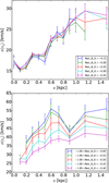 |
Fig. 5 Influence of the adopted metallicity ranges for the thin (top) and thick (bottom) disk RC samples on the intrinsic vertical velocity dispersions (for the default realization). For the thick disk velocity dispersion profile only there is a dependence on the adopted upper metallicity boundary, partly due to contamination by the low metallicity tail of the thin disk. The bins plotted are fully independent (non-overlapping). |
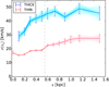 |
Fig. 6 Mean intrinsic vertical velocity dispersion profile over all realizations for both the thin metal-rich (red) and thick metal-poor (blue) disk RC stars. The error bars show the spread over all realizations due to the spread in the absolute magnitude of the RC stars and as a result of the error deconvolution. |
3.2.2 The Kz force
Because our goal is to measure the contribution of dark matter more reliably, we focus on the bins at large Galactic heights, since for small z the baryons (are expected to) dominate the gravitational force. We thus choose to explore only those bins for which the central z-coordinate satisfies |z|≥ 0.6 kpc.
We are now ready to insert the moments (and their errors) in Eq. (5). This equation also requires knowledge of the variation of σ(vz) with z. Rather than differentiating the data directly, we fit a linear function to σ(vz) as function of z, whose slope and uncertainty are then used in Eq. (5).
To compute Kz, we set R = R⊙ in the last term of Eq. (5), and we fix the scale lengths of both disks to an intermediate value of 2.5 kpc (e.g. Siegel et al. 2002; Jurić et al. 2008; Bensby et al. 2011; McMillan 2011; Bovy et al. 2012; Robin et al. 2012, 2014; Bland-Hawthorn & Gerhard 2016). Finally we explore how Kz varies for a set of scale heights for the thin and thick disk populations.
Figure 7 shows the derived vertical forces in black for  kpc and
  kpc. The solid line corresponds to the thin disk sample, the dashed line to the thick disk sample. Since we folded our data towards positive z, the forces derived are negative. We find
 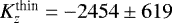 (km s−1)2 kpc−1 and
 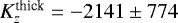 (km s−1)2 kpc−1 at 1.5 kpc away from the Galactic plane. We also show the decomposition of Kz into the three terms of Eq.(5): the first associated with vertical velocity dispersion (blue), the second with the slope of the vertical variance as function of z (green), and the third with the mixed velocity moment (red). The first term dominates Kz for both samples. In addition, we find that the error on Kz is dominated by that on the vertical velocity dispersion for the thin disk sample, while for the thick disk it is the error on the slope.
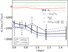 |
Fig. 7 Derived vertical force Kz (black lines) for the thin (solid lines) and the thick disk samples (dashed lines). The coloured lines show the decomposition of Kz into the terms concerning the vertical velocity dispersion (blue), the slope of the vertical variance as function of z (green), and the mixed velocity moment (red). The curves shown were computed for the combination |


3.3 Massmodel
Now that wedetermined Kz, and hence the total surface mass density Σ(z) according to Eq. (2) (which is strictly equivalent only if we assume ∂(RFR)∕∂R = 0 for all z), we proceed to compare it to the surface mass density derived from the contribution of all baryonic components and explore the need for dark matter.
We characterize the baryonic components with a double exponential stellar thin and thick disk, and an infinitely thin ISM disk with a surface mass density equal to 13 M⊙ pc−2 (Holmberg & Flynn 2000), and consider a constant dark matter density3. We further fix the midplane stellar density at the solar radius to 0.043 M⊙ pc−3 (McKee et al. 2015), which is very similar to the value of (0.040 ± 0.002) M⊙ pc−3 found by Bovy (2017). We fix the midplane thick-to-thin disk density ratio to 12% (Jurić et al. 2008)4.
To explore the effect of the assumed thin and thick disk scale heights on the local dark matter density estimates, we sample the thin disk scale height from 200 to 400 pc and the thick disk scale height from 700 to 1300 pc, such that typical estimates reported in the literature are covered (e.g. Bland-Hawthorn & Gerhard 2016). For each combination we determine the value of ρDM by minimizing the total χ2-value defined as
 (8)
(8)
where j runs over all data points for which surface mass densities have been derived for both the thin and thick disk data. The best-fit model thus minimizes jointly  , but to understand the quality of the models, we inspect separately the reduced
  and
and  .
.
The results for various combinations of scale height parameters are shown in Fig. 8. In the left panel we show the χ2 values as functions of the local dark matter density parameter for a number of models. The thick black curve shows the case of a model with scale heights  and
and  kpc. This is the model with the lowest χ2 among all the different combinations explored. The dashed horizontal line corresponds to Δ χ2 = 1.0 with respect to its minimum value, which is the criterion we use to quantify the error on the dark matter density determination. In this panel we also show (from orange to dark red) the χ2 curves for models with varying thin disk scale height for fixed
  kpc. Models with fixed
  kpc, but with varying thick disk scale height are given with colours varying from light to dark blue. We thus see that a relatively large change in thick disk scale height does not alter the inferred dark matter density by much, although Δ χ2 > 1 for, for example
  kpc. On the other hand, a small change in the thin disk scale height has a large influence on the inferred dark matter density.
This is also depicted in the right panel of Fig. 8, where we show the best-fit dark matter densities for all combinations of scale heights explored. The green star indicates the location in  -space where the model can fit the data the best. The larger impact of the thin disk scale height on the fitted dark matter density is probably driven by the smaller error bars on the gravitational force profile implied from the thin disk sample in comparison to that from the thick disk sample (see e.g. Fig. 6). Yellow lines indicate where the total baryonic surface mass density in the models equals 35, 40, 45, 50, and 55 M⊙ pc−2. Most previous works seem to agree on baryonic surface mass densities in the range 40− 55 M⊙ pc−2 (e.g. McKee et al. 2015, and references therein), thus the models with combinations of scale heights that result in smaller or larger baryonic contributions are less plausible.
In Fig. 9 we explore further the quality of the fits obtained by comparing the reduced χ2 values as computed from the thin (left) and thick disk data (right). The panels show that the thin disk data is always fitted well, but that models with a very low (or large) thin and large (or low) thick disk scale height do not lead to a high quality fit for the thick disk data.
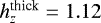
In summary, the model and data are thus most consistent for  kpc and
  kpc, which results in Σbaryon = 44.8 M⊙ pc−2. In this case, the inferred local dark matter density is 0.018 ± 0.002 M⊙ pc−3. This model is shown in Fig. 10 and has χ2 = 2.6. With 11 degrees of freedom (12 data points and 1 model parameter), this value implies that the quality of the fit is good. We note that the uncertainty on the scale heights of the populations used constitute a much larger source of error on the estimate of the local dark matter density than the measurement errors alone, which lead to a relative error of order 10% only.
In the analysis presented thus far we considered all data within |R − R⊙|≤ 0.5 kpc. When we restrict ourselves to a smaller volume, within 0.25 kpc from R⊙, the dataset is smaller and this leads to less constraining power, especially for the thick disk set, on the value of the local dark matter density. For this more local sample, we find that the model does not fit the thin disk data well ( ) for
) for  kpc and for the thick disk if
 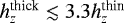 .
.
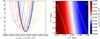 |
Fig. 8 Left: χ2 values as functions of the local dark matter density for various combinations of the scale heights of the thin and thick disks. The (light to dark) blue curves have |

![Mathematical equation: $h_z^{\textrm{thick}}=\left[0.85,0.94,1.03,1.21,1.30\right]$](/articles/aa/full_html/2018/07/aa32903-18/aa32903-18-eq54.png)
![Mathematical equation: $h_z^{\textrm{thin}}=\left[0.22,0.24,0.26,0.27,0.29,0.30,0.32,0.34\right]$](/articles/aa/full_html/2018/07/aa32903-18/aa32903-18-eq55.png)


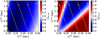 |
Fig. 9 Maps of the reduced χ2 values computed for the thin (left) and thick (right) disk samples separately. The thin disk sample is generally fitted well with the minimization of the joint χ2, and this is because it contributes with a larger number of data points with smaller error bars. This is not the case for the thick disk, where for certain combinations of the scale heights the fit is poor for this sample ( |
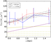 |
Fig. 10 Surface mass density as implied from the axisymmetric Jeans equation, derived for the thin (red) and thick (blue) disk samples. In this example the scale height for the thin disk tracer stars (red) is set to 0.28 kpc, the scale height for the thick disk tracer stars (blue) to 1.12 kpc. This combination of parameters gives the lowest χ2 value (see Fig. 8) when fitting our mass model (black), which is the sum of the baryonic (solid yellow) components (thin, ISM, and thick disks from top to bottom in dashed yellow) and the dark matter component (purple). |
4 Conclusions
We have studied the kinematics of RC stars from the RAVExTGAS dataset. The kinematic maps obtained are well behaved, do not show evidence for strong bending or breathing modes up to 0.7 kpc from the midplane, and only show a small hint of radial motions towards the outer disk. We therefore applied the axisymmetric Jeans equation relating kinematic moments to the vertical force, ultimately yielding a new measurement of the dark matter density in the solar neighbourhood. To account for the presence of multiple populations, we divided the RC sample into thin and thick disk tracer samples according to the metallicity of the stars, as estimated from the RAVE dataset, and fitted both populations simultaneously. This allowed us to determine a local value of the dark matter density with a relative internal error (due to measurement errors on the observables) of only 13.5%, ρDM(R⊙, 0) = 0.018 ± 0.002 M⊙ pc−3, which is in reasonable agreement with previous work.
It is however misleading to consider only the internal errors on the dark matter density, as they do not account for the large systematic uncertainties in the stellar disk parameters (especially the scale heights), the thick-to-thin disk density ratio, the scale lengths of the disks, and the ISM mass. These (external) sources of uncertainty can lead to a large systematic error on the dark matter density near the Sun. For example a 10% difference in the scale height of the thin disk leads to a 30% change in the value of ρDM, and a nearly equally good fit to the data. The change due to uncertainties on the scale height of the thick disk is slightly weaker. It is therefore extremely important to get accurate constraints on the stellar disk parameters of the tracer stars used. Future Gaia data releases will characterize better and more precisely the various stellar components in the Galaxy, and thus allow a more global and accurate approach to determining the contribution of the dark matter, not just locally, but also as a function of position in the Galactic disk.
Acknowledgements
We thank the referee, Dr. Chris Flynn, for his very prompt and constructive report. We also thank M.A. Breddels, D. Massari, L. Posti, and J. Veljanoski for numerous discussions. A.H. acknowledges financial support from a VICI grant from The Netherlands Organisation for Scientific Research, N.W.O. This work has made use of data from the European Space Agency (ESA) mission Gaia (https://www.cosmos.esa.int/gaia), processed by the Gaia Data Processing and Analysis Consortium (DPAC, https://www.cosmos.esa.int/web/gaia/dpac/consortium). Funding for the DPAC has been provided by national institutions, in particular the institutions participating in the Gaia Multilateral Agreement. Funding for RAVE has been provided by the following institutions: the Australian Astronomical Observatory; the Leibniz-Institut fuer Astrophysik Potsdam (AIP); the Australian National University; the Australian Research Council; the French National Research Agency; the German Research Foundation (SPP 1177 and SFB 881); the European Research Council (ERC-StG 240271 Galactica); the Istituto Nazionale di Astrofisica at Padova; The Johns Hopkins University; the National Science Foundation of the USA (AST-0908326); the W. M. Keck foundation; the Macquarie University; the Netherlands Research School for Astronomy; the Natural Sciences and Engineering Research Council of Canada; the Slovenian Research Agency; the Swiss National Science Foundation; the Science & Technology Facilities Council of the UK; Opticon; Strasbourg Observatory; and the Universities of Groningen, Heidelberg and Sydney. The RAVE web site is at https://www.rave-survey.org.
References
- Allende Prieto, C., Kawata, D., & Cropper, M. 2016, A&A, 596, A98 [NASA ADS] [CrossRef] [EDP Sciences] [Google Scholar]
- Banik, N., Widrow, L. M., & Dodelson, S. 2017, MNRAS, 464, 3775 [NASA ADS] [CrossRef] [Google Scholar]
- Bedding, T. R., Mosser, B., Huber, D., et al. 2011, Nature, 471, 608 [NASA ADS] [CrossRef] [PubMed] [Google Scholar]
- Bensby, T., Alves-Brito, A., Oey, M. S., Yong, D., & Meléndez, J. 2011, ApJ, 735, L46 [NASA ADS] [CrossRef] [Google Scholar]
- Bienaymé, O., Famaey, B., Siebert, A., et al. 2014, A&A, 571, A92 [NASA ADS] [CrossRef] [EDP Sciences] [Google Scholar]
- Binney, J., Gerhard, O., & Spergel, D. 1997, MNRAS, 288, 365 [NASA ADS] [CrossRef] [Google Scholar]
- Bland-Hawthorn, J., & Gerhard, O. 2016, ARA&A, 54, 529 [NASA ADS] [CrossRef] [EDP Sciences] [Google Scholar]
- Bovy, J. 2017, MNRAS, 470, 1360 [NASA ADS] [CrossRef] [Google Scholar]
- Bovy, J., & Tremaine, S. 2012, ApJ, 756, 89 [Google Scholar]
- Bovy, J., Rix, H.-W., Liu, C., et al. 2012, ApJ, 753, 148 [NASA ADS] [CrossRef] [Google Scholar]
- Büdenbender, A., van de Ven, G., & Watkins, L. L. 2015, MNRAS, 452, 956 [NASA ADS] [CrossRef] [Google Scholar]
- Carrillo, I., Minchev, I., Kordopatis, G., et al. 2018, MNRAS, 475, 2679 [NASA ADS] [CrossRef] [Google Scholar]
- Casetti-Dinescu, D. I., Girard, T. M., Korchagin, V. I., & van Altena W. F. 2011, ApJ, 728, 7 [NASA ADS] [CrossRef] [Google Scholar]
- Chaplin, W. J., & Miglio, A. 2013, ARA&A, 51, 353 [NASA ADS] [CrossRef] [Google Scholar]
- Cui, X.-Q., Zhao, Y.-H., Chu, Y.-Q., et al. 2012, Res. Astron. Astrophys., 12, 1197 [NASA ADS] [CrossRef] [Google Scholar]
- ESA 1997, ESA SP, 1200 [Google Scholar]
- Foreman-Mackey, D., Hogg, D. W., Lang, D., & Goodman, J. 2013, PASP, 125, 306 [CrossRef] [Google Scholar]
- Gaia Collaboration (Brown, A. G. A., et al.) 2016a, A&A, 595, A2 [NASA ADS] [CrossRef] [EDP Sciences] [Google Scholar]
- Gaia Collaboration (Prusti, T., et al.) 2016b, A&A, 595, A1 [NASA ADS] [CrossRef] [EDP Sciences] [Google Scholar]
- Girardi, L. 2016, ARA&A, 54, 95 [NASA ADS] [CrossRef] [EDP Sciences] [Google Scholar]
- Groenewegen, M. A. T. 2008, A&A, 488, 935 [NASA ADS] [CrossRef] [EDP Sciences] [Google Scholar]
- Hawkins, K., Leistedt, B., Bovy, J., & Hogg, D. W. 2017, MNRAS, 471, 722 [NASA ADS] [CrossRef] [Google Scholar]
- Helmi, A., Veljanoski, J., Breddels, M. A., Tian, H., & Sales, L. V. 2017, A&A, 598, A58 [NASA ADS] [CrossRef] [EDP Sciences] [Google Scholar]
- Hessman, F. V. 2015, A&A, 579, A123 [NASA ADS] [CrossRef] [EDP Sciences] [Google Scholar]
- Holmberg, J., & Flynn, C. 2000, MNRAS, 313, 209 [NASA ADS] [CrossRef] [Google Scholar]
- Jurić, M., Ivezić, Ž., Brooks, A., et al. 2008, ApJ, 673, 864 [NASA ADS] [CrossRef] [MathSciNet] [Google Scholar]
- Kuijken, K., & Gilmore, G. 1989, MNRAS, 239, 571 [NASA ADS] [CrossRef] [Google Scholar]
- Kunder, A., Kordopatis, G., Steinmetz, M., et al. 2017, AJ, 153, 75 [NASA ADS] [CrossRef] [Google Scholar]
- Lewis, J. R., & Freeman, K. C. 1989, AJ, 97, 139 [NASA ADS] [CrossRef] [Google Scholar]
- Liang, X. L., Zhao, J. K., Oswalt, T. D., et al. 2017, ApJ, 844, 152 [NASA ADS] [CrossRef] [Google Scholar]
- Lindegren, L., Lammers, U., Bastian, U., et al. 2016, A&A, 595, A4 [NASA ADS] [CrossRef] [EDP Sciences] [Google Scholar]
- Majewski, S. R., Schiavon, R. P., Frinchaboy, P. M., et al. 2017, AJ, 154, 94 [NASA ADS] [CrossRef] [Google Scholar]
- McKee, C. F., Parravano, A., & Hollenbach, D. J. 2015, ApJ, 814, 13 [NASA ADS] [CrossRef] [Google Scholar]
- McMillan, P. J. 2011, MNRAS, 414, 2446 [NASA ADS] [CrossRef] [Google Scholar]
- McMillan, P. J., Kordopatis, G., Kunder, A., et al. 2018, MNRAS, 477, 5279 [NASA ADS] [CrossRef] [Google Scholar]
- Monari, G., Kawata, D., Hunt, J. A. S., & Famaey, B. 2017, MNRAS, 466, L113 [NASA ADS] [CrossRef] [Google Scholar]
- Moni Bidin, C., Carraro, G., Méndez, R. A., & Smith, R. 2012, ApJ, 751, 30 [NASA ADS] [CrossRef] [Google Scholar]
- Moni Bidin, C., Smith, R., Carraro, G., Méndez, R. A., & Moyano, M. 2015, A&A, 573, A91 [NASA ADS] [CrossRef] [EDP Sciences] [Google Scholar]
- Paczyński, B., & Stanek, K. Z. 1998, ApJ, 494, L219 [NASA ADS] [CrossRef] [Google Scholar]
- Piffl, T., Binney, J., McMillan, P. J., et al. 2014, MNRAS, 445, 3133 [NASA ADS] [CrossRef] [Google Scholar]
- Read, J. I. 2014, J. Phys. G: Nucl. Phys., 41, 063101 [Google Scholar]
- Reid, M. J., Menten, K. M., Brunthaler, A., et al. 2014, ApJ, 783, 130 [Google Scholar]
- Robin, A. C., Marshall, D. J., Schultheis, M., & Reylé, C. 2012, A&A, 538, A106 [NASA ADS] [CrossRef] [EDP Sciences] [Google Scholar]
- Robin, A. C., Reylé, C., Fliri, J., et al. 2014, A&A, 569, A13 [NASA ADS] [CrossRef] [EDP Sciences] [Google Scholar]
- Ruiz-Dern, L., Babusiaux, C., Arenou, F., Turon, C., & Lallement, R. 2018, A&A, 609, A116 [NASA ADS] [CrossRef] [EDP Sciences] [Google Scholar]
- Salucci, P., Nesti, F., Gentile, G., & Frigerio Martins C. 2010, A&A, 523, A83 [NASA ADS] [CrossRef] [EDP Sciences] [Google Scholar]
- Schönrich, R. 2012, MNRAS, 427, 274 [NASA ADS] [CrossRef] [Google Scholar]
- Schönrich, R., Binney, J., & Dehnen, W. 2010, MNRAS, 403, 1829 [NASA ADS] [CrossRef] [Google Scholar]
- Siebert, A., Famaey, B., Minchev, I., et al. 2011, MNRAS, 412, 2026 [NASA ADS] [CrossRef] [Google Scholar]
- Siegel, M. H., Majewski, S. R., Reid, I. N., & Thompson, I. B. 2002, ApJ, 578, 151 [NASA ADS] [CrossRef] [Google Scholar]
- Silverwood, H., Sivertsson, S., Steger, P., Read, J. I., & Bertone, G. 2016, MNRAS, 459, 4191 [CrossRef] [Google Scholar]
- Sivertsson, S., Silverwood, H., Read, J. I., Bertone, G., & Steger, P. 2018, MNRAS, 478, 1677 [Google Scholar]
- van der Kruit,P. C., & Searle, L. 1982, A&A, 110, 61 [Google Scholar]
- Widrow, L. M., Gardner, S., Yanny, B., Dodelson, S., & Chen, H.-Y. 2012, ApJ, 750, L41 [NASA ADS] [CrossRef] [Google Scholar]
- Williams, M. E. K., Steinmetz, M., Binney, J., et al. 2013, MNRAS, 436, 101 [NASA ADS] [CrossRef] [Google Scholar]
- Yu, J., & Liu, C. 2018, MNRAS, 475, 1093 [NASA ADS] [CrossRef] [Google Scholar]
In the analysis carried out below we find ⟨vR ⟩ = 5.8 ± 3.3 km s−1 and ⟨vz ⟩ = −0.6 ± 1.9 km s−1, for the thick disk, and 1.4 ± 1.1 and 0.5 ± 0.6 km s−1, respectively, for the thin disk RC stars in our sample (at large heights).
We find that the difference in the amplitude of Kz for a spherically aligned ellipsoid or one where cov(vR, vz) varies as σ2(vR) and σ2 (vz), is less than 10% of the uncertainty on Kz due to measurement errors.
The assumption of a constant dark matter density is a reasonable approximation for the volume probed by our data, since for example the difference in surface mass density with an NFW halo with a scale radius of 14.4 kpc and a flattening 0.9 as in Piffl et al. (2014), is only ~1% at z = 1.5 kpc.
Varying this ratio has a minor impact on the results described in this section, as factor two decrease leads to an increase in ρDM of only 4.5%.
All Figures
|
Fig. 1 Selection and calibration of RC stars. Left: distribution of giant stars in our sample in the extinction-corrected colour vs. surface gravity space. The blue lines enclose our RC sample. Right: extinction-corrected HR diagram of stars in our sample. The solid and dashed light blue lines indicate the adopted mean and standard deviation of the RC absolute KS -band magnitude, respectively. |
| In the text | |
|
Fig. 2 Meridional plane RC star counts in bins of 0.5 kpc in R and 0.1 kpc in z (as indicated by the box in the upper right corner). The white contours indicate where the number of RC stars in the bins have dropped to 200, 100, and 50 from inner to outer contours respectively. The black symbol marks the position of the Sun. This figure is based on the default realization in which the absolute magnitudes of all RC stars are set to
|
| In the text | |
|
Fig. 3 Mean velocities of RC stars in the meridional plane based on the default realization in which the absolute magnitudes of all RC stars are set to |
| In the text | |
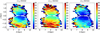 |
Fig. 4 Similar to Fig. 3, but now showing the standard deviation of the velocities. |
| In the text | |
|
Fig. 5 Influence of the adopted metallicity ranges for the thin (top) and thick (bottom) disk RC samples on the intrinsic vertical velocity dispersions (for the default realization). For the thick disk velocity dispersion profile only there is a dependence on the adopted upper metallicity boundary, partly due to contamination by the low metallicity tail of the thin disk. The bins plotted are fully independent (non-overlapping). |
| In the text | |
|
Fig. 6 Mean intrinsic vertical velocity dispersion profile over all realizations for both the thin metal-rich (red) and thick metal-poor (blue) disk RC stars. The error bars show the spread over all realizations due to the spread in the absolute magnitude of the RC stars and as a result of the error deconvolution. |
| In the text | |
|
Fig. 7 Derived vertical force Kz (black lines) for the thin (solid lines) and the thick disk samples (dashed lines). The coloured lines show the decomposition of Kz into the terms concerning the vertical velocity dispersion (blue), the slope of the vertical variance as function of z (green), and the mixed velocity moment (red). The curves shown were computed for the combination |
| In the text | |
|
Fig. 8 Left: χ2 values as functions of the local dark matter density for various combinations of the scale heights of the thin and thick disks. The (light to dark) blue curves have |
| In the text | |
|
Fig. 9 Maps of the reduced χ2 values computed for the thin (left) and thick (right) disk samples separately. The thin disk sample is generally fitted well with the minimization of the joint χ2, and this is because it contributes with a larger number of data points with smaller error bars. This is not the case for the thick disk, where for certain combinations of the scale heights the fit is poor for this sample ( |
| In the text | |
|
Fig. 10 Surface mass density as implied from the axisymmetric Jeans equation, derived for the thin (red) and thick (blue) disk samples. In this example the scale height for the thin disk tracer stars (red) is set to 0.28 kpc, the scale height for the thick disk tracer stars (blue) to 1.12 kpc. This combination of parameters gives the lowest χ2 value (see Fig. 8) when fitting our mass model (black), which is the sum of the baryonic (solid yellow) components (thin, ISM, and thick disks from top to bottom in dashed yellow) and the dark matter component (purple). |
| In the text | |
Current usage metrics show cumulative count of Article Views (full-text article views including HTML views, PDF and ePub downloads, according to the available data) and Abstracts Views on Vision4Press platform.
Data correspond to usage on the plateform after 2015. The current usage metrics is available 48-96 hours after online publication and is updated daily on week days.
Initial download of the metrics may take a while.