| Issue |
A&A
Volume 615, July 2018
|
|
|---|---|---|
| Article Number | A167 | |
| Number of page(s) | 9 | |
| Section | Catalogs and data | |
| DOI | https://doi.org/10.1051/0004-6361/201832678 | |
| Published online | 03 August 2018 | |
Probing narrow-line Seyfert 1 galaxies in the southern hemisphere⋆
1
Dipartimento di Fisica e Astronomia “G. Galilei”, Università di Padova, Vicolo dell’Osservatorio 3, 35122 Padova, Italy
e-mail: This email address is being protected from spambots. You need JavaScript enabled to view it.
2
Center for Astrophysics, Guangzhou University, 510006 Guangzhou, PR China
3
Istituto Nazionale di Fisica Nucleare (INFN), Sezione di Padova, 35131 Padova, Italy
4
INAF – Osservatorio Astronomico di Brera, Via E. Bianchi 46, 23807 Merate (LC), Italy
5
INAF – Osservatorio Astronomico di Padova, Vicolo dell’Osservatorio 5, 35122 Padova, Italy
6
Dipartimento di Fisica e Astronomia “G. Galilei”, Università di Padova, Via Marzolo 8, 35131 Padova, Italy
Received:
21
January
2018
Accepted:
17
April
2018
Abstract
We present a new accurate catalog of narrow-line Seyfert 1 galaxies (NLS1s) in the southern hemisphere from the Six-degree Field Galaxy Survey (6dFGS) final data release, which is currently the most extensive spectroscopic survey available in the southern sky whose database has not yet been systematically explored. We classified 167 sources as NLS1s based on their optical spectral properties. We derived flux-calibrated spectra for the first time that the 6dFGS does not provide. By analyzing these spectra, we obtained strong correlations between the monochromatic luminosity at 5100 Å and the luminosities of Hβ and [O III]λ5007 lines. The central black hole mass and the Eddington ratio have average values of 8.6 × 10⁶M⊙ and 0.96 LEdd respectively, which are typical values for NLS1s. In the sample, 23 (13.8%) NLS1s were detected at radio frequencies, and 12 (7.0%) of them are radio-loud. Our results confirmed that radio-loud sources tend to have higher redshift, a more massive black hole, and higher radio and optical luminosities than radio-quiet sources.
Key words: galaxies: active / galaxies: nuclei / galaxies: Seyfert / quasars: emission lines / quasars: supermassive black holes
Tables 1, 2, 4, and 5 are only available at the CDS via anonymous ftp to cdsarc.u-strasbg.fr (130.79.128.5) or via http://cdsarc.u-strasbg.fr/viz-bin/qcat?J/A+A/615/A167
© ESO 2018
1. Introduction
Narrow-line Seyfert 1 galaxies (NLS1s) are a well-known sub-class of active galactic nuclei (AGN). The classification is based on their optical spectral properties. Their Hβ lines, originating in the broad-line region (BLR), have by definition a full width at half maximum FWHM (Hβ) < 2000 km s−1, and a flux ratio of [O III]λ5007 / Hβ < 3 (Osterbrock & Pogge 1985; Goodrich 1989). Most of their optical spectra show strong Fe II multiplets emission, which is a sign that the BLR and the accretion disk are visible (Mullaney & Ward 2008; Pogge 2011). These narrow permitted lines are commonly interpreted as a low rotational velocity around a relatively undermassive central black hole compared to broad-line Seyfert 1 galaxies (BLS1s), typically in the ranges of MBH ~ 106−8M⊙ for NLS1s and MBH ~ 107−8M⊙ for BLS1s (Mathur 2000). This leads to the conclusion that NLS1s have a high Eddington ratio, from 0.1 to 1 or even above (Boroson & Green 1992; Collin & Kawaguchi 2004). The low black hole mass and high accretion rate suggest that NLS1s might be a young and fast-growing phase of AGN (Mathur 2000; Grupe 2000). In this scenario, NLS1s might be different with respect to BLS1s, as suggested by their different large-scale environments: NLS1s preferably reside in less dense environments than BLS1s (Järvelä et al. 2017). Another possible interpretation is that the narrowness of Hβ lines in NLS1s might be due to the pole-on orientation of a disk-like BLR, which prevents us from seeing any Doppler broadening (Jolley & Kuncic 2008). In this case, the low black hole mass of NLS1s is not real, but only an inclination effect. However, our current knowledge is too poor to reach a conclusion.
Some NLS1s are detected at radio frequencies. The radio properties of AGN are usually described by the radio-loudness parameter, which is defined as the flux ratio between 5 GHz and optical B-band, RL = F5GHz/FB-band. Sources with RL > 10 are considered as radio-loud (RL), while the others belong to radio-quiet (RQ) population (Kellermann et al. 1989). Among radio-detected NLS1s, the majority of them are RQ, while only a fraction of NLS1s are RL (7%) or very RL (2.5%) with a radio-loudness RL > 100 (Komossa et al. 2006). The RL fraction of NLS1s is indeed half of the fraction of RL quasars (15%) (Kellermann et al. 1989). However, this fraction strongly depends on the redshift since it appears to be lower in the nearby universe (Cracco et al. 2016), and relies on the large-scale environment as it tends to be higher with increasing large-scale environment density (Järvelä et al. 2017). These RL NLS1s generally have a very compact radio morphology (Gu & Chen 2010; Doi et al. 2012). Instead, RQ NLS1s usually exhibit an extended emission (Berton et al. 2018).
The discovery of γ-ray emission from NLS1s detected by the Fermi γ-ray Space Telescope confirmed that NLS1s are the third class of AGN emitting γ-rays from a relativistic beamed jet, in addition to blazars and radio galaxies (Abdo et al. 2009). However only a handful of sources are detected at γ-rays. The physical properties of NLS1s are different from those of blazars and radio galaxies. The central black hole masses of NLS1s are on average one to two orders of magnitude lower than those of blazars and radio galaxies. This difference might be due to a projection effect in the inclination scenario. Moreover, NLS1s are generally hosted in spiral galaxies (Crenshaw et al. 2003), while blazars and radio galaxies are both typically hosted in elliptical galaxies (Sikora et al. 2007). If we assume that the young age scenario is correct, RL NLS1s might be the progenitors of flat spectrum radio quasars (FSRQs; Foschini et al. 2015; Berton et al. 2016).
To have a better understanding of the nature of NLS1s, observations with advanced observing facilities will be necessary. NLS1s are typically fainter with respect to blazars and quasars, and RL NLS1s are especially tricky since they are usually located at relatively high redshift. Some new facilities, such as the Extremely Large Telescope (ELT), the Atacama Large Millimeter/submillimeter Array (ALMA), and the Square Kilometre Array (SKA), could make a great contribution in providing break-through evidence to solve many long lasting problems concerning this particularly intriguing class of AGN. However, most of these large telescopes are concentrated in the southern hemisphere. Therefore the aim of this work is to create a new NLS1 sample that can be observed by large telescopes in the southern hemisphere, for the purpose of investigating the peculiarity of NLS1s with respect to other AGN. To do this, we exploited the large unexplored archive of the Six-degree Field Galaxy Survey (6dFGS)1, and provided flux calibration to their spectra for the first time.
Throughout this work, we adopt a standard ΛCDM cosmology with a Hubble constant H0 = 70 km s−1 Mpc−1, ΩΛ = 0.73 and ΩM = 0.27 (Komatsu et al. 2011). We assume the flux density and spectral index convention Fv ∝ v−αv.
2. Sample selection
The spectral data of the NLS1 sample are derived from the 6dFGS, which is a combined redshift and peculiar velocity survey over the entire southern sky with |b| > 10°. Optical spectra were obtained through separate V and R gratings and later spliced to produce combined spectra spanning 4000 Å–7500 Å. The instrumental resolution is R ~ 1000 (Jones et al. 2004). The third and final data release (DR3) for the 6dFGS was published on 1 April 2009 (Jones et al. 2009).
We analyzed 110880 archive spectra from the 6dFGS DR3 catalog. They were first corrected for redshift using the cz velocity parameter (km s−1) provided by the catalog. The continuum was fitted in two wavelength intervals (4725 Å–4775 Å and 5075 Å–5125 Å) that do not show strong emission line, and subtracted from the original spectra. The root mean square (RMS) was calculated in the regions mentioned above as well. We selected objects showing strong Hβ and [O III] lines, based on the criterion that the peak of each emission line has to be larger than 3·RMS. In this case, we found 38 563 objects that having both emission lines.
We then calculated the FWHM of these emission lines. The Hβ line was fitted with three Gaussians (one narrow component and two broad components), the [O III] line was fitted with two Gaussians (one narrow component and one broad component), and both of them were corrected for instrumental resolution (300 km s−1 for the 6dFGS). The narrow component is the line core and the broad components are usually associated with the gas outflow. An example of continuum subtraction and emission lines Gaussian fitting is shown in Fig. 1.
 |
Fig. 1. Spectrum of 6dFGS gJ135439.5-421457. The green line is the observed spectrum, the blue line is the continuum, the red line is the spectrum after the continuum subtraction, and the black line is the result of fitting Hβ with three Gaussians and [O III] with two Gaussians. Data are taken from the 6dFGS. |
After reproducing the line profiles, we applied two additional conditions on the FWHM of lines. The first one was 600 km s−1 < FWHM(Hβ) < 2200 km s−1. The lower limit is based on the mean FWHM of emission lines from the narrow-line region (NLR) measured by Vaona et al. (2012), and the upper limit was defined by the classic 2000 km s−1 criterion with a 10 % tolerance (Cracco et al. 2016). The second condition was 200 km s−1 < FWHM([O III]) < 2000 km s−1. The lower limit avoids contamination by cosmic rays, while the upper limit avoids loss of objects with strong Fe II multiplets and relatively weak [O III] line (Osterbrock & Pogge 1985; Mullaney et al. 2013). The fluxes of the Hβ and [O III] lines were measured by integrating the fitted profiles. We only focused on those objects with a flux ratio of [O III] / Hβ < 3, which is a main feature of NLS1s (Osterbrock & Pogge 1985).
Based on the criteria mentioned above, we selected 2126 spectra and further analyzed them one by one to discern NLS1s from intermediate Seyfert galaxies and low-ionization nuclear emission-line regions (LINERs). Intermediate Seyfert galaxies and LINERs also have narrow emission lines and a flux ratio of [O III] / Hβ < 3 (Osterbrock 1977; Veilleux & Osterbrock 1987). However, there are two features in the spectra of NLS1s that distinguish them from the others. On one hand, Fe II multiplets are usually present in the spectra, because the BLR, where Fe II multiplets are originated, is directly visible in type 1 AGN. On the other hand, the line profile of Hβ is broader than [O III] and can be fitted with a Lorentzian profile caused by turbulence in the line emitting region (Kollatschny & Zetzl 2013). The differences between NLS1s, intermediate Seyfert galaxies, and LINERs can be seen in Fig. 2.
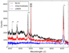 |
Fig. 2. Three spectral examples showing the differences between a NLS1 6dFGS gJ123124.9-165350 (black line), an intermediate Seyfert galaxy 6dFGS gJ072957.1-654333 (red line), and a LINER 6dFGS gJ160558.2-263806 (blue line). Data are taken from the 6dFGS. |
In this way, we obtained a new sample of 167 NLS1s in the southern hemisphere. The object’s name, coordinates, redshift, and luminosity distance are reported in Table 1; FWHM and flux of Hβ and [O III] lines are listed in Table 2. The range of redshift is from z = 0.01 (DL = 44.49 Mpc) to z = 0.50 (DL = 2825.63 Mpc) with an average value of z = 0.15 (DL = 767.40 Mpc). The redshift distribution of the sample is presented in Fig. 3.
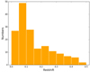 |
Fig. 3. Redshift distribution of 167 NLS1s using a 0.05 bin width |
3. Flux calibration
Spectra from the 6dFGS are not flux-calibrated, therefore a method to calibrate the spectra in the sample is needed. We looked for NLS1s that are both in the 6dFGS sample and observed by the Sloan Digital Sky Survey (SDSS), based on a coordinates match between the 6dFGS and the SDSS spectroscopic database, within a tolerance radius of 0.1 arcmin. The images of the sources in both surveys were compared to make sure that the search resulted in the same sources that we were looking for. As a result, seven NLS1s observed by both the 6dFGS and the SDSS were selected for the flux calibration.
We also checked that these objects are not RL to reduce the effects of optical variability. This is because RL sources are found to have higher variability than RQ sources due to the presence of non-thermal emission coming from the relativistic jet along with thermal emission related to the accretion disk around the supermassive black hole in RL objects, compared to the contribution of only thermal emission from the accretion disk in RQ objects (Rakshit & Stalin 2017).
We calculated the ratio between counts and flux for each object, dividing the 6dFGS spectra by the SDSS spectra, then combined the results and averaged them using the IRAF V2.16. The sensitivity of the 6dFGS NLS1 sample was obtained by fitting the average ratio with a fifth order polynomial curve. The average counts/flux ratio and the sensitivity are shown in Fig. 4. The airmass was considered in a crude correction for all data using the standard stars Feige 110 and EG 274 in the 6dFGS observations (Jones et al. 2004). Hence, we calibrated the NLS1 spectra in the sample using the sensitivity obtained above. The spectra of these 167 NLS1s were then corrected for galactic extinction using the AV extinction coefficients (Landolt V) (Schlafly & Finkbeiner 2011) extracted from the NASA/IPAC2 Extragalactic Database (NED)3, and shifted to the rest frame. In this way we obtained flux-calibrated spectra for the NLS1 sample.
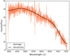 |
Fig. 4. Average counts/flux ratio (red line) and sensitivity (black line) of the 6dFGS NLS1 sample. |
An issue with the method we used to calibrate the spectra is that the sensitivity was calculated on a limited number of objects, because of the small common sky coverage of the 6dFGS and the SDSS. In order to examine whether the flux calibration is acceptable, we compared the relation between the continuum flux and the optical magnitude of our 6dFGS re-calibrated spectra with that of NLS1s flux-calibrated spectra selected by Cracco et al. (2016), who investigated a sample of 296 NLS1s from the SDSS Data Release (DR) 7.
We performed averaged flux measurements running on the wavelength range from 5050 Å to 5150 Å, to obtain the mean flux at 5100 Å for both the 6dFGS and SDSS samples. The magnitude on B-band of the 6dFGS sample is provided by the catalog. The SDSS, instead, gives the magnitude of photometric measurements in the ugriz system. Hence, we converted the magnitude on g and r bands for the objects in the SDSS sample into magnitude on B-band using the equation (Jester et al. 2005) (1)
(1)
The magnitudes were also corrected for galactic extinction in both samples.
The relation between the mean flux at 5100 Å and the magnitude on B-band for the 6dFGS and SDSS samples is shown in Fig. 5. The best fit for the 6dFGS sample is (2)
(2)
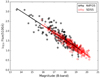 |
Fig. 5. Relation of the mean flux at 5100 Å and the magnitude on B-band. The black stars and line are data from the 6dFGS sample, the red circles and line are data from the SDSS sample in Cracco et al. (2016). |
which is comparable with the one for the SDSS sample expressed by (3)
(3)
Based on the consistent properties of our re-calibrated 6dFGS spectra with respect to the full flux-calibrated SDSS spectra, we infer that the derived sensitivity provides a realistic solution, though introducing some degrees of uncertainty. The magnitude on B-band and the mean flux density at 5100 Å of the 6dFGS NLS1 sample are listed in Table 1.
We carried out an additional test for our flux calibration. Sources with a declination higher than −15° and apparent magnitude brighter than 18 and 19 can be observed by the Asiago Astrophysical Observatory (Italy) 1.22 m and 1.82 m telescopes respectively. We observed 15 objects’ optical spectra in the 6dFGS sample using these telescopes in October and November 2017 in the best seeing conditions of 1” (details are reported in Table 3). The observations were split into exposure times of 1200 s or 1800 s for each target to avoid strong contamination by cosmic rays and light pollution. The wavelength calibration done by FeAr or NeHgAr lamps. Standard stars HR7596, HR9087, or HD2857, whose altitude close to the target, was used for the flux calibration. After the sky subtraction, we combined the spectra for each object, and corrected for galactic absorption and redshift.
We compared the flux-calibrated spectra obtained from the 6dFGS and the Asiago telescopes. Two examples are shown in Fig. 6. In spite of the fact that the sources used to create the sensitivity are not RL, we do expect some variations and the most critical effect on the thermal blue bump. On the other hand, differences on the red part can be well accounted for by the different aperture and seeing conditions. Thus even though the uncertainties on the blue and red extremes of the spectral range are not negligible, the fluxes around the Hβ line, [O III] line, and 5100 Å continuum regions are consistent. Hence we suppose that for our purpose the flux calibration result is reliable, and these regions can be used to calculate the black hole mass and the Eddington ratio.
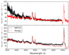 |
Fig. 6. Top panel: flux-calibrated spectra of 6dFGS gJ021218.3-073720 obtained from the 6dFGS (black line) and the Asiago 1.22 m Telescope (red line). Bottom panel: flux-calibrated spectra of 6dFGS gJ045557.5-145641 obtained from the 6dFGS (black line) and the Asiago 1.82 m Telescope (red line). |
Observational details of the Asiago optical spectra.
4. Luminosity correlation
Working with spectra produced by a multi-object spectrograph, and fed by a system of fixed aperture entrance fibers, we have to account for the amount of light that enters the instrument. On one hand, we think about the nuclear active regions of external galaxies as unresolved point-like sources, the aperture of the 6dFGS instrument fibers is large enough to avoid the loss of significant amounts of light. On the other hand, the use of a fixed aperture implies that a varying amount of light from the AGN host galaxy, which can be an extended source with resolved structure, is also collected by the instrument. For strong type 1 AGN, which dominate over the host, this problem is not particularly relevant, but it can represent a significant issue in the case of nearby resolved Seyfert galaxies (Varisco et al. 2018). In general, this problem does not affect the spectral components that are purely originated by the AGN, such as the broad emission lines, while we have to take it into account when measuring the intensity of continuum, and to some extent, the narrow emission lines.
In fact, estimating the host galaxy contribution in such spectra is not straightforward, because the relative amount of host galaxy stellar light with respect to the AGN signal, depends both on the AGN luminosity and on the fraction of the host surface that is subtended by the aperture that increases as a square of distance. To evaluate the contribution of stellar light from host galaxies in our sample, we applied a technique based on the principal component analysis (PCA), which was originally described in Connolly et al. (1995), and subsequently applied to a sample of type 1 AGN selected from the SDSS DR3 by La Mura et al. (2007). Following the strategy described in La Mura et al. (2007), we assume that the observed spectra can be regarded as the linear combination of a set of spectral contributions, arising separately from the AGN and its host. If we call S (λ) the amount of flux observed at a wavelength λ, this leads us to write (4)
(4)
where Ai(λ) and Hj(λ) represent the spectral components produced by the AGN and its host respectively, ai and hj are their weight coefficients that do not depend on wavelength, and n and m are the number of linear components used to model the AGN and its host. Using a proper set of base spectra, such as the list of eigenspectra provided by the low redshift collections in Yip et al. (2004 a,b), Eq. (4) expands to a system of algebraic equations that can be solved in terms of the weight coefficients. Therefore we can estimate the contribution of AGN and host galaxy components in the spectra, after they have been corrected for galactic extinction and brought to their rest frame.
As the simple solution of Eq. (4) may not always lead to a physically meaningful conclusion, because it introduces negative spectra or absorption features corresponding to forbidden lines, we developed an iterative fitting procedure written in Python. The algorithm looks for the solution of Eq. (4), then it tests for the physical meaning of the separated AGN and host spectra. If either one of the components exhibits any inconsistency, its weight is reduced and the fit is run again leaving only the consistent parts free to vary. The algorithm then proceeds with an iteration fitting AGN and host alternatively, which are now forced to show only non-negative contributions, until the solution converges to a minimum chi-square χ2 value or one of the components becomes undetected. After testing various configurations, we found that the best fit models leaving minimum residuals could be obtained from the combination of the first n AGN and the first m host galaxy components. Two examples of AGN and host galaxy decompositions are shown in Fig. 7.
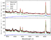 |
Fig. 7. Decompositions of AGN and host galaxy in spectra 6dFGS gJ065017.5-380514 (top panel) and 6dFGS gJ084510.2-073205 (bottom panel). The black line shows the observed spectrum, the red line shows the best-fitted result, the green line shows the AGN component, and the blue line shows the stellar contribution. |
The procedure is generally able to recover the host galaxy contribution, producing models with a median reduced residual of χ2 = 1.45 estimated over the sample. In a dozen cases, the host contribution turned out to be too faint to be distinguished. In all the other cases, we subtracted the host galaxy spectral models from our flux-calibrated spectra, in order to obtain an estimate of the light originally emitted by the AGN alone. After the host galaxy correction, the monochromatic luminosity at 5100 Å can be calculated by (5)
(5)
where DL is the luminosity distance estimated by the cosmological redshift, F(λ) is the averaged flux density on the wavelength range from 5050 Å to 5150 Å, and we assume that the radiation from the sources is isotropic. The luminosity at 5100 Å may be overestimated in RL NLS1s due to the presence of relativistic jets can contaminate the continuum in RL sources. However, this impact is negligible, since only a small fraction of NLS1s are RL as mentioned above.
From the host galaxy subtractions, we noted that the stellar light has an important influence on the continuum, however, it only makes a minor contribution to the emission lines, since we did not see any strong emission or absorption line in the host galaxy components. Therefore, the luminosities of Hβ and [O III] lines can be estimated based on the fluxcalibrated spectra. We first subtracted the continuum from the spectra, then fitted the Fe II multiplets and subtracted them from the continuum-subtracted spectra. The Fe II templates were estimated using the procedure described in Kovačević et al. (2010), Shapovalova et al. (2012). It reproduces 65 Fe II emission lines within the 4000 Å to 5500 Å range, including five line groups (F, S, G, P, I Zw 1), and fits each line with a single Gaussian. The free input parameters are temperature, Doppler width, shift, intensity of each group of lines, and iterations4. An example of Fe II multiplets fitting is shown in Fig. 8.
 |
Fig. 8. he Fe II multiplets fitting in spectrum 6dFGS gJ003915.9-511702. Top panel: continuum-subtracted spectrum (red line) and Fe II template (black line). Bottom panel: spectrum after subtraction of both continuum and Fe II multiplets (green line). Data are taken from the 6dFGS. |
We used the spectra with both the continuum and the Fe II multiplets subtracted to estimate the fluxes and luminosities of Hβ and [O III] lines. The signal-to-noise (S/N) ratio was computed from 5050 Å to 5150 Å wavelength range. If S/N > 10, the Hβ line was fitted with three Gaussians (one narrow component and two broad components). Otherwise it was fitted with two Gaussians (one narrow component and one broad component), in order to avoid overfitting the noise in the case of low quality spectra. The [O III] line was fitted with two Gaussians. The luminosities of Hβ and [O III] lines is calculated by (6)
(6)
where F(line) is the flux derived by integrating the Hβ and [O III] line profiles.
The luminosity at 5100 Å, and the luminosities of Hβ and [O III] lines for the 6dFGS NLS1 sample are reported in Table 4. We obtained strong correlations between the monochromatic luminosity at 5100 Å and the luminosities of both emission lines as shown in Fig. 9. The linear regressions with a Bayesian method yield (Kelly 2007)
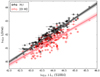 |
Fig. 9. Relation of L(Hβ)–λLλ (5100 Å) is shown in black stars and lines. Relation of L([O III])–λLλ (5100 Å) is shown in red circles and lines. |
 (7)
(7)
and (8)
(8)
A strong correlation between the luminosity of Balmer lines and the optical continuum was found by Greene & Ho (2005), Greene et al. (2010), and supports the idea that the Balmer emission lines arise from recombination after photoionization by non-thermal continuum (Yee 1980). Zhou et al. (2006) also found a correlation between the luminosity of [O III] line and the optical continuum, although not as tight as the L(Hβ) – λLλ (5100 Å) correlation. This relation is useful for estimating the intrinsic luminosity of AGN, since the unobscured NLR, where the [O III] line comes from, can be reliably used to trace the central region properties (Zakamska et al. 2003).
The errors of flux and luminosity of continuum were obtained by calculating their standard deviation σ from 5050 Å to 5150 Å. The errors of FWHM, flux, and luminosity of emission lines were evaluated by the Monte Carlo method. This approach involves varying the line profiles with a random noise proportional to the RMS measured in the continuum range, then fitting the emission lines with Gaussians as previously mentioned, measuring FWHM, flux, and luminosity, and repeating the same process 100 times to estimate their standard deviation. In this way, we obtained 1σ errors for these parameters.
5. Black hole mass and Eddington ratio
We estimated the central black hole mass following the method in Foschini et al. (2015) and Berton et al. (2015). For each NLS1 galaxy in the 6dFGS sample, the virial mass of the central black hole is defined as (9)
(9)
where RBLR is the size of the BLR measured by reverberation or estimated from scaling relations, σline is the line dispersion second-order moment, G is the gravitational constant, and f is a dimensionless scale factor that depends on the structure, kinematics, and orientation of the BLR (Peterson et al. 2004). We assumed f = 4.31 ± 1.05 following Grier et al. (2013), which is a value not dependent on the inclination and geometry of the BLR.
The size of the BLR was calculated using the relation between the luminosity at 5100 Å and the radius of the BLR from Bentz et al. (2013), (10)
(10)
The line dispersion σHβ, which is less affected by the inclination and line profile than a FWHM measurement (Peterson et al. 2004; Collin et al. 2006), was determined from the Hβ broad components. If the Hβ line has two broad components, the σHβ is evaluated by (11)
(11)
where F(λ) is the Hβ line profile produced by two broad components. If it has only one broad component, then σHβ ≃ FWHMHβbroad / 2.355.
The Eddington ratio, defined as ∈ = Lbol/LEdd, could be measured after obtaining the central black hole mass, where the Eddington luminosity is (12)
(12)
and the bolometric luminosity is estimated assuming Lbol = 9 λLλ (5100 Å) (Kaspi et al. 2000).
The distributions of central black hole mass and Eddington ratio for 167 NLS1s in the 6dFGS sample are plotted in Fig. 10, and their estimated values are presented in Table 4. The masses of the central black hole MBH range from 8.1 × 10⁵M⊙ to 7.8×10⁷M⊙ with a median value of 8.6×10⁶M⊙. The Eddington ratios Lbol/LEdd span from 0.07 to 5.35 with a median value of 0.96. This result confirms that NLS1s have lower black hole mass and higher Eddington ratio than BLS1s. The errors of central black hole mass and Eddington ratio were evaluated by the Python uncertainties package following the error propagation theory.
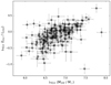 |
Fig. 10. Distributions of central black hole mass and Eddington ratio in the 6dFGS NLS1 sample. |
6. Radio sources
With the aim of looking for radio sources in the 6dFGS sample, we subsequently cross-matched these 167 NLS1s with several important radio surveys covering the southern hemisphere, including the NRAO VLA5 Sky Survey (NVSS), the Sydney University Molonglo Sky Survey (SUMSS), and the Australia Telescope 20 GHz Survey (AT20G), within a search radius of 5 arcsec. The NVSS covers the entire sky north of −40° declination at 1.4 GHz with the flux density limit of 2.5 mJy (Condon et al. 1998), the SUMSS covers the sky south of −30° declination at 843 MHz with the flux density limit of 8 mJy (Mauch et al. 2003), and the AT20G covers the whole sky south of 0° declination at 5 GHz, 8.4 GHz, and 22 GHz respectively, with the flux density limit of 40 mJy (Murphy et al. 2010).
We found 18 sources only detected by the NVSS, three sources only detected by the SUMSS, one source detected by both the NVSS and the SUMSS, and one source detected by both the SUMSS and the AT20G. In total 23 (13.8%) sources have associated radio counterparts. The flux densities detected by the radio surveys for these 23 sources are listed in Table 5 respectively.
The radio loudness RL = Fradio/Foptical was calculated using the radio flux at 5 GHz and the optical flux at B-band 4400 Å for each object. In most cases the radio flux was obtained at 1.4 GHz and 843 MHz instead of 5 GHz. We derived the radio flux at 5 GHz under the hypothesis that the radio spectrum can be described with a power-law model Fv ∝ v−α, and we assumed a conservative spectral index of α = 0.5 (Yuan et al. 2008). In this way we found 12 (7.0% of the whole sample) RL (including one very RL) NLS1s and 11 RQ NLS1s. If we suppose that the radio spectrum has a flat spectral index of α = 0, 17 objects were found to be RL and six objects were found to be RQ. Instead, assuming a steep radio spectral index of α = 1, we found that seven objects are RL and 16 objects are RQ. In this paper, we classified our sources according to the results of α = 0.5.
Williams et al. (2002) analyzed 150 NLS1s in the SDSS Early DR and found that only a dozen (8%) were detected at radio frequencies and only two (1.3%) were RL. Research by Zhou et al. (2006) based on the SDSS DR3 resulted in a sample of 2011 NLS1s and of those 142 (7.1%) objects had radio counterparts. Cracco et al. (2016) investigated a sample of 296 NLS1s from the SDSS DR7, 70 (23.6%) sources were detected at radio frequencies and 11 (3.7% of the total sample and 15.7% of those radio detected) of them were classified as RL. A recent study by Rakshit et al. (2017) proposed a new catalog from the SDSS DR12 that contains 11101 NLS1s, among them 555 (5%) objects were detected on radio band and 378 (3.4%) were RL.
The radio fraction is different in all these samples because the radio loudness strongly depends on the spatial resolution of the optical and radio observations. The flux is different if the observations considered the whole galaxy (including the contribution of both AGN and host) or only the nuclear region. Then the evaluated RL is different for the same galaxy. This situation happens both on radio and optical observations. Ho & Peng (2001) found that most Seyfert 1 nuclei were classified as RL AGN if only their nuclear luminosity was considered, which was in doubt later.
The classification of RL and RQ according to RL = 10 is not restricted and a little arbitrary. In light of this, a recent work by Padovani (2017) argued that AGN should be classified based on physical differences rather than just an observational phenomenon. They defined two new classes of AGN: jetted AGN, which are characterized by strong relativistic jets, and non-jetted AGN, which also have jet structures but with weak power compared to those of jetted sources. The spectral energy distribution (SED) of non-jetted AGN has a cutoff at much lower energy than jetted AGN. Despite this, the radio-loudness parameter has been useful to separate RL sources from RQ ones until now.
The flux densities and luminosities on radio and optical bands, radio loudness, and radio type of the radio sample are reported in Table 5. The mean values of redshift, black hole mass, radio luminosity at 5 GHz, and optical luminosity on B-band of the RL and RQ subsamples are presented in Table 6. Their number and cumulative distributions are shown in Figs. 11, 12, 13 and 14 respectively.
Mean values of redshift, black hole mass, radio luminosity at 5 GHz, and optical luminosity on B-band of the RL and RQ subsample
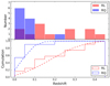 |
Fig. 11. Redshift distribution (top panel) and cumulative distribution (bottom panel) of the RL (red) and RQ (blue) sources in our radio detected NLS1 sample using a 0.05 bin width. |
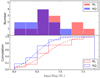 |
Fig. 12. Black hole mass distribution (top panel) and cumulative distribution (bottom panel) of the RL (red) and RQ (blue) sources as in previous figure using a 0.25 bin width. |
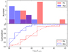 |
Fig. 13. Radio luminosity at 5 GHz distribution (top panel) and cumulative distribution (bottom panel) of the RL (red) and RQ (blue) sources as in previous figure using a 0.5 bin width. |
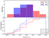 |
Fig. 14. Optical luminosity on B-band distribution (top panel) and cumulative distribution (bottom panel) of the RL (red) and RQ (blue) sources as in previous figure using a 0.5 bin width. |
We used the two-sample Kolmogorov–Smirnov (K–S) test to examine whether the parent population of the RL and RQ sub-sample is the same. The null hypothesis is that two distributions originated from the same population of sources. We applied the rejection of the null hypothesis at a 95% confidence level corresponding to a value of p ≤ 0.05. The K–S tests of redshift (p = 1.8 × 10⁻³) and radio luminosity (p = 2.0 × 10⁻⁴) suggest that the RL and RQ NLS1s in the sample have different populations. However, the K–S tests of black hole mass (p = 0.47) and optical luminosity (p = 0.055) argue that these RL and RQ sources have the same origin.
This result is expected. The different redshift distribution may be caused by a selection effect. RQ sources are faint, so they can be observed only at low redshift due to the flux density limit of radio surveys. Once the redshift increases, only RL sources with high luminosity can be detected. The different radio luminosity distribution may be related to the presence of radio jets. RL NLS1s generally harbor relativistic jets, instead jets in RQ NLS1s are usually weak or absent. However, the optical luminosity and black hole mass distributions have the same origin, the possible reason is that the optical luminosity is emitted by the accretion disk and the black hole mass is derived from the optical continuum in this analysis. This result also implies that the presence of relativistic jets is not related to the central black hole mass.
The cumulative distributions of the radio sample show as well that RL sources tend to have higher redshift, a more massive black hole, and higher radio and optical luminosity than RQ sources on average. This may be related to the jet activity. RL NLS1s usually harbor relativistic jets emitting low-energy synchrotron radiation (radio emission) and high-energy inverse-Compton radiation (up to σ-ray energy). Instead jets are probably weak or absent in RQ NLS1s. The mass accretion rate of sources with jets is higher than that of sources without jets. Since the presence of jets enhances angular momentum transport, matter in the accretion disk loses angular momentum and falls into the central black hole faster. This can greatly increases the black hole mass growth rate, therefore RL sources have larger black hole masses and higher luminosities compared to RQ sources (Jolley & Kuncic 2008). Finally, we remark that these results should be taken with cautions because of the small radio sample used in these analyses.
7. Summary
In this work, we exploited the optical spectra from the 6dFGS DR3, which is currently the most extensive spectroscopic survey available in the southern hemisphere, to perform the first systematic selection of NLS1s in this sky region. The NLS1 sample was selected from this survey and flux calibration for the optical spectra in the sample was derived. The luminosity correlations of L(Hβ) – λLλ (5100 Å) and L([O III]) – λLλ (5100 Å) were found. The central black hole mass and the Eddington ratio were estimated for each target. In addition, the radio counter-parts were found for some sources by the radio surveys covering the southern hemisphere. The main results of this paper are summarized as follows.
-
According to the criteria of 600 km s−1 < FWHM(Hβ) < 2200 km s−1 and a flux ratio of [O III] / Hβ < 3, as well as considering the visibility of Fe II multiplets and Hβ line profiles in the optical spectra, we created a new accurate sample of 167 NLS1s from the 6dFGS in the southern hemisphere.
-
The flux-calibrated spectra for these 167 NLS1s in the sample, which were not provided by the 6dFGS, were obtained. To evaluate the reliability of the flux calibration, the relation between the mean flux at 5100 Å and the magnitude on B-band was calculated for the 6dFGS sample, and the result is in good agreement with the SDSS NLS1 sample from Cracco et al. (2016). We further compared 15 flux-calibrated spectra in the 6dFGS sample with the new observations specifically carried out at the Asiago Observatory, and confirmed that our flux calibration of the 6dFGS spectra on the Hβ line, [O III] line, and 5100 Å continuum regions is consistent.
-
The monochromatic luminosity at 5100 Å, and the luminosities of Hβ and [O III] lines were estimated. Strong correlations of L(Hβ) – λLλ (5100 Å) and L([O III]) – λLλ (5100 Å) could be confirmed.
-
The mass of central black hole and the Eddington ratio were calculated for each target, and found to lie in the ranges of MBH ~ 105.91−7.89M⊙ and Lbol/LEdd ~ 0.07−5.35 respectively, with average values of MBH = 106.93M⊙ and Lbol/LEdd = 0.96, which are typical values for NLS1s. This result confirms that NLS1s have lower black hole mass and higher Eddington ratio than BLS1s.
-
Of the 167 NLS1s in the 6dFGS sample, 23 (13.8%) sources were found to have associated radio counterparts, including 12 (7.0%) RL NLS1s and 11 RQ NLS1s. RL sources tend to have higher redshift, a more massive black hole, and higher radio and optical luminosities than RQ sources.
Our conclusions increase the number of NLS1s and confirm some well known properties of this peculiar class of AGN. However, the number of NLS1s in the 6dFGS sample, in particular radio sources, is still limited. Further research with larger samples, and higher resolution and sensitivity observations will be necessary to understand the physical mechanism and evolution of NLS1s, with respect to other types of AGN. We expect that the investigation of these sources with high performance observation facilities, located in the southern sites, will help to clarify many of the fundamental questions that have not yet been solved on this class of galaxies.
Acknowledgments
We thank the anonymous referee for suggestions leading to the improvement of this work. JHFan’s work is partially supported by the National Natural Science Foundation of China (NSFC 11733001, U1531245). We thank the Final Data Release (DR3) of the Six-degree Field Galaxy Survey (6dFGS). Funding for the Sloan Digital Sky Survey IV has been provided by the Alfred P. Sloan Foundation, the US Department of Energy Office of Science, and the Participating Institutions. SDSS-IV acknowledges support and resources from the Center for High-Performance Computing at the University of Utah. The SDSS web site is www.sdss.org. SDSS-IV is managed by the Astrophysical Research Consortium for the Participating Institutions of the SDSS Collaboration including the Brazilian Participation Group, the Carnegie Institution for Science, Carnegie Mellon University, the Chilean Participation Group, the French Participation Group, Harvard-Smithsonian Center for Astrophysics, Instituto de Astrofísica de Canarias, the Johns Hopkins University, Kavli Institute for the Physics and Mathematics of the Universe (IPMU) / University of Tokyo, Lawrence Berkeley National Laboratory, Leibniz Institut für Astrophysik Potsdam (AIP), Max-Planck-Institut für Astronomie (MPIA Heidelberg), Max-Planck-Institut für Astrophysik (MPA Garching), Max-Planck-Institut für Extraterrestrische Physik (MPE), National Astronomical Observatories of China, New Mexico State University, New York University, University of Notre Dame, Observatário Nacional / MCTI, the Ohio State University, Pennsylvania State University, Shanghai Astronomical Observatory, United Kingdom Participation Group, Universidad Nacional Autónoma de México, University of Arizona, University of Colorado Boulder, University of Oxford, University of Portsmouth, University of Utah, University of Virginia, University of Washington, University of Wisconsin, Vanderbilt University, and Yale University. This research has made use of the NASA/IPAC Extragalactic Database (NED), which is operated by the Jet Propulsion Laboratory, California Institute of Technology, under contract with the National Aeronautics and Space Administration. This paper is based on observations collected with the 1.22 m Galileo and 1.82 m Copernico telescopes of the Asiago Astrophysical Observatory, operated by the Department of Physics and Astronomy “G. Galilei” of the University of Padova and INAF – Osservatorio Astronomico di Padova. This research has made use of the VizieR catalog access tool, CDS, Strasbourg, France. The original description of the VizieR service was published in Ochsenbein et al. (2000).
The National Aeronautics and Space Administration / The Infrared Processing and Analysis Center.
The National Radio Astronomy Observatory Very Large Array.
References
- Abdo, A. A., Ackermann, M., Ajello, M., et al. 2009, ApJ, 707, L142 [NASA ADS] [CrossRef] [Google Scholar]
- Bentz, M. C., Denney, K. D., Grier, C. J., et al. 2013, ApJ, 767, 149 [NASA ADS] [CrossRef] [Google Scholar]
- Berton, M., Foschini, L., Ciroi, S., et al. 2015, A&A, 578, A28 [NASA ADS] [CrossRef] [EDP Sciences] [Google Scholar]
- Berton, M., Caccianiga, A., Foschini, L., et al. 2016, A&A, 591, A98 [NASA ADS] [CrossRef] [EDP Sciences] [Google Scholar]
- Berton, M., Congiu, E., Järvelä, E., et al. 2018, A&A, 614, A87 [NASA ADS] [CrossRef] [EDP Sciences] [Google Scholar]
- Boroson, T. A., & Green, R. F. 1992, ApJS, 80, 109 [NASA ADS] [CrossRef] [Google Scholar]
- Collin, S., & Kawaguchi, T. 2004, A&A, 426, 797 [NASA ADS] [CrossRef] [EDP Sciences] [Google Scholar]
- Collin, S., Kawaguchi, T., Peterson, B. M., & Vestergaard, M. 2006, A&A, 456, 75 [NASA ADS] [CrossRef] [EDP Sciences] [Google Scholar]
- Condon, J. J., Cotton, W. D., Greisen, E. W., et al. 1998, AJ, 115, 1693 [NASA ADS] [CrossRef] [Google Scholar]
- Connolly, A. J., Szalay, A. S., Bershady, M. A., Kinney, A. L., & Calzetti, D. 1995, AJ, 110, 1071 [NASA ADS] [CrossRef] [Google Scholar]
- Cracco, V., Ciroi, S., Berton, M., et al. 2016, MNRAS, 462, 1256 [NASA ADS] [CrossRef] [Google Scholar]
- Crenshaw, D. M., Kraemer, S. B., & Gabel, J. R. 2003, AJ, 126, 1690 [NASA ADS] [CrossRef] [Google Scholar]
- Decarli, R., Dotti, M., Fontana, M., & Haardt, F. 2008, MNRAS, 386, L15 [NASA ADS] [Google Scholar]
- Doi, A., Nagira, H., Kawakatu, N., et al. 2012, ApJ, 760, 41 [NASA ADS] [CrossRef] [Google Scholar]
- Foschini, L., Berton, M., Caccianiga, A., et al. 2015, A&A, 575, A13 [NASA ADS] [CrossRef] [EDP Sciences] [Google Scholar]
- Goodrich, R. W. 1989, ApJ, 342, 224 [NASA ADS] [CrossRef] [Google Scholar]
- Greene, J. E., & Ho, L. C. 2005, ApJ, 630, 122 [NASA ADS] [CrossRef] [Google Scholar]
- Greene, J. E., Hood, C. E., Barth, A. J., et al. 2010, ApJ, 723, 409 [NASA ADS] [CrossRef] [Google Scholar]
- Grier, C. J., Martini, P., Watson, L. C., et al. 2013, ApJ, 773, 90 [CrossRef] [Google Scholar]
- Grupe, D. 2000, New Astron. Rev., 44, 455 [NASA ADS] [CrossRef] [Google Scholar]
- Gu, M., & Chen, Y. 2010, AJ, 139, 2612 [NASA ADS] [CrossRef] [Google Scholar]
- Ho, L. C., & Peng, C. Y. 2001, ApJ, 555, 650 [NASA ADS] [CrossRef] [Google Scholar]
- Järvelä, E., Lähteenmäki, A., Lietzen, H., et al. 2017, A&A, 606, A9 [NASA ADS] [CrossRef] [EDP Sciences] [Google Scholar]
- Jester, S., Schneider, D. P., Richards, G. T., et al. 2005, AJ, 130, 873 [NASA ADS] [CrossRef] [Google Scholar]
- Jolley, E. J. D., & Kuncic, Z. 2008, MNRAS, 386, 989 [NASA ADS] [CrossRef] [Google Scholar]
- Jones, D. H., Saunders, W., Colless, M., et al. 2004, MNRAS, 355, 747 [NASA ADS] [CrossRef] [Google Scholar]
- Jones, D. H., Read, M. A., Saunders, W., et al. 2009, MNRAS, 399, 683 [NASA ADS] [CrossRef] [Google Scholar]
- Kaspi, S., Smith, P. S., Netzer, H., et al. 2000, ApJ, 533, 631 [NASA ADS] [CrossRef] [Google Scholar]
- Kellermann, K. I., Sramek, R., Schmidt, M., Shaffer, D. B., & Green, R. 1989, AJ, 98, 1195 [NASA ADS] [CrossRef] [Google Scholar]
- Kelly, B. C. 2007, ApJ, 665, 1489 [NASA ADS] [CrossRef] [Google Scholar]
- Kollatschny, W., & Zetzl, M. 2013, A&A, 549, A100 [NASA ADS] [CrossRef] [EDP Sciences] [Google Scholar]
- Komatsu, E., Smith, K. M., Dunkley, J., et al. 2011, ApJS, 192, 18 [NASA ADS] [CrossRef] [Google Scholar]
- Komossa, S., Voges, W., Xu, D., et al. 2006, AJ, 132, 531 [NASA ADS] [CrossRef] [Google Scholar]
- Kovačević, J., Popović, L. Č., & Dimitrijević, M. S. 2010, ApJS, 189, 15 [NASA ADS] [CrossRef] [Google Scholar]
- La Mura, G., Popović, L. Č., Ciroi, S., Rafanelli, P., & Ilić, D. 2007, ApJ, 671, 104 [NASA ADS] [CrossRef] [Google Scholar]
- Mathur, S. 2000, MNRAS, 314, L17 [NASA ADS] [CrossRef] [Google Scholar]
- Mauch, T., Murphy, T., Buttery, H. J., et al. 2003, MNRAS, 342, 1117 [NASA ADS] [CrossRef] [Google Scholar]
- Mullaney, J. R., & Ward, M. J. 2008, MNRAS, 385, 53 [NASA ADS] [CrossRef] [Google Scholar]
- Mullaney, J. R., Alexander, D. M., Fine, S., et al. 2013, MNRAS, 433, 622 [NASA ADS] [CrossRef] [Google Scholar]
- Murphy, T., Sadler, E. M., Ekers, R. D., et al. 2010, MNRAS, 402, 2403 [NASA ADS] [CrossRef] [Google Scholar]
- Ochsenbein, F., Bauer, P., & Marcout, J. 2000, A&AS, 143, 23 [NASA ADS] [CrossRef] [EDP Sciences] [Google Scholar]
- Osterbrock, D. E. 1977, ApJ, 215, 733 [NASA ADS] [CrossRef] [Google Scholar]
- Osterbrock, D. E., & Pogge, R. W. 1985, ApJ, 297, 166 [NASA ADS] [CrossRef] [Google Scholar]
- Padovani, P. 2017, Nature Astronomy, 1, 0194 [Google Scholar]
- Peterson, B. M., Ferrarese, L., Gilbert, K. M., et al. 2004, ApJ, 613, 682 [NASA ADS] [CrossRef] [Google Scholar]
- Pogge, R. W. 2011, in Narrow-Line Seyfert 1 Galaxies and their Place in the Universe, 2 [Google Scholar]
- Rakshit, S., & Stalin, C. S. 2017, ApJ, 842, 96 [NASA ADS] [CrossRef] [Google Scholar]
- Rakshit, S., Stalin, C. S., Chand, H., & Zhang, X.-G. 2017, ApJS, 229, 39 [NASA ADS] [CrossRef] [Google Scholar]
- Schlafly, E. F., & Finkbeiner, D. P. 2011, ApJ, 737, 103 [NASA ADS] [CrossRef] [Google Scholar]
- Shapovalova, A. I., Popović, L. Č., Burenkov, A. N., et al. 2012, ApJS, 202, 10 [NASA ADS] [CrossRef] [Google Scholar]
- Sikora, M., Stawarz, Ł., & Lasota, J.-P. 2007, ApJ, 658, 815 [NASA ADS] [CrossRef] [Google Scholar]
- Vaona, L., Ciroi, S., Di Mille, F., et al. 2012, MNRAS, 427, 1266 [NASA ADS] [CrossRef] [Google Scholar]
- Varisco, L., Sbarrato, T., Calderone, G., & Dotti, M. 2018, A&A, in press, DOI: 10.1051/0004-6361/201832655 [EDP Sciences] [Google Scholar]
- Veilleux, S., & Osterbrock, D. E. 1987, ApJS, 63, 295 [NASA ADS] [CrossRef] [Google Scholar]
- Williams, R. J., Pogge, R. W., & Mathur, S. 2002, AJ, 124, 3042 [NASA ADS] [CrossRef] [Google Scholar]
- Yee, H. K. C. 1980, ApJ, 241, 894 [NASA ADS] [CrossRef] [Google Scholar]
- Yip, C. W., Connolly, A. J., Szalay, A. S., et al. 2004a, AJ, 128, 585 [NASA ADS] [CrossRef] [Google Scholar]
- Yip, C. W., Connolly, A. J., Vanden Berk, D. E., et al. 2004b, AJ, 128, 2603 [NASA ADS] [CrossRef] [Google Scholar]
- Yuan, W., Zhou, H. Y., Komossa, S., et al. 2008, ApJ, 685, 801 [NASA ADS] [CrossRef] [Google Scholar]
- Zakamska, N. L., Strauss, M. A., Krolik, J. H., et al. 2003, AJ, 126, 2125 [NASA ADS] [CrossRef] [Google Scholar]
- Zhou, H., Wang, T., Yuan, W., et al. 2006, ApJS, 166, 128 [NASA ADS] [CrossRef] [Google Scholar]
All Tables
Mean values of redshift, black hole mass, radio luminosity at 5 GHz, and optical luminosity on B-band of the RL and RQ subsample
All Figures
|
Fig. 1. Spectrum of 6dFGS gJ135439.5-421457. The green line is the observed spectrum, the blue line is the continuum, the red line is the spectrum after the continuum subtraction, and the black line is the result of fitting Hβ with three Gaussians and [O III] with two Gaussians. Data are taken from the 6dFGS. |
| In the text | |
|
Fig. 2. Three spectral examples showing the differences between a NLS1 6dFGS gJ123124.9-165350 (black line), an intermediate Seyfert galaxy 6dFGS gJ072957.1-654333 (red line), and a LINER 6dFGS gJ160558.2-263806 (blue line). Data are taken from the 6dFGS. |
| In the text | |
|
Fig. 3. Redshift distribution of 167 NLS1s using a 0.05 bin width |
| In the text | |
|
Fig. 4. Average counts/flux ratio (red line) and sensitivity (black line) of the 6dFGS NLS1 sample. |
| In the text | |
|
Fig. 5. Relation of the mean flux at 5100 Å and the magnitude on B-band. The black stars and line are data from the 6dFGS sample, the red circles and line are data from the SDSS sample in Cracco et al. (2016). |
| In the text | |
|
Fig. 6. Top panel: flux-calibrated spectra of 6dFGS gJ021218.3-073720 obtained from the 6dFGS (black line) and the Asiago 1.22 m Telescope (red line). Bottom panel: flux-calibrated spectra of 6dFGS gJ045557.5-145641 obtained from the 6dFGS (black line) and the Asiago 1.82 m Telescope (red line). |
| In the text | |
|
Fig. 7. Decompositions of AGN and host galaxy in spectra 6dFGS gJ065017.5-380514 (top panel) and 6dFGS gJ084510.2-073205 (bottom panel). The black line shows the observed spectrum, the red line shows the best-fitted result, the green line shows the AGN component, and the blue line shows the stellar contribution. |
| In the text | |
|
Fig. 8. he Fe II multiplets fitting in spectrum 6dFGS gJ003915.9-511702. Top panel: continuum-subtracted spectrum (red line) and Fe II template (black line). Bottom panel: spectrum after subtraction of both continuum and Fe II multiplets (green line). Data are taken from the 6dFGS. |
| In the text | |
|
Fig. 9. Relation of L(Hβ)–λLλ (5100 Å) is shown in black stars and lines. Relation of L([O III])–λLλ (5100 Å) is shown in red circles and lines. |
| In the text | |
|
Fig. 10. Distributions of central black hole mass and Eddington ratio in the 6dFGS NLS1 sample. |
| In the text | |
|
Fig. 11. Redshift distribution (top panel) and cumulative distribution (bottom panel) of the RL (red) and RQ (blue) sources in our radio detected NLS1 sample using a 0.05 bin width. |
| In the text | |
|
Fig. 12. Black hole mass distribution (top panel) and cumulative distribution (bottom panel) of the RL (red) and RQ (blue) sources as in previous figure using a 0.25 bin width. |
| In the text | |
|
Fig. 13. Radio luminosity at 5 GHz distribution (top panel) and cumulative distribution (bottom panel) of the RL (red) and RQ (blue) sources as in previous figure using a 0.5 bin width. |
| In the text | |
|
Fig. 14. Optical luminosity on B-band distribution (top panel) and cumulative distribution (bottom panel) of the RL (red) and RQ (blue) sources as in previous figure using a 0.5 bin width. |
| In the text | |
Current usage metrics show cumulative count of Article Views (full-text article views including HTML views, PDF and ePub downloads, according to the available data) and Abstracts Views on Vision4Press platform.
Data correspond to usage on the plateform after 2015. The current usage metrics is available 48-96 hours after online publication and is updated daily on week days.
Initial download of the metrics may take a while.