| Issue |
A&A
Volume 615, July 2018
|
|
|---|---|---|
| Article Number | A124 | |
| Number of page(s) | 14 | |
| Section | Interstellar and circumstellar matter | |
| DOI | https://doi.org/10.1051/0004-6361/201732391 | |
| Published online | 25 July 2018 | |
Structure of X-ray emitting jets close to the launching site: from embedded to disk-bearing sources⋆
1
S. D. Astronomía y Geodesia, Facultad de Ciencias Matemáticas, Universidad Complutense de Madrid, 28040
Madrid, Spain
e-mail: This email address is being protected from spambots. You need JavaScript enabled to view it.
2
INAF-Osservatorio Astronomico di Palermo, Piazza del Parlamento 1, 90134 Palermo, Italy
3
Dipartimento di Fisica e Chimica, Università di Palermo, Via Archirafi 36, 90123 Palermo, Italy
Received:
1
December
2017
Accepted:
15
March
2018
Abstract
Context. Several observations of stellar jets show evidence of X-ray emitting shocks close to the launching site. In some cases, including young stellar objects (YSOs) at different stages of evolution, the shocked features appear to be stationary. We study two cases, both located in the Taurus star-forming region. HH 154, the jet originating from the embedded binary Class 0/I protostar IRS 5, and the jet associated with DG Tau, a more evolved Class II disk-bearing source or classical T Tauri star (CTTS).
Aims. We investigate the effect of perturbations in X-ray emitting stationary shocks in stellar jets and the stability and detectability in X-rays of these shocks, and we explore the differences in jets from Class 0 to Class II sources.
Methods. We performed a set of 2.5D magnetohydrodynamic numerical simulations that model supersonic jets ramming into a magnetized medium. The jet is formed of two components: a continuously driven component that forms a quasi-stationary shock at the base of the jet and a pulsed component consisting of blobs perturbing the shock. We explored different parameters for the two components. We studied two cases: HH 154, a light jet (less dense than the ambient medium), and a heavy jet (denser than the ambient medium) associated with DG Tau. We synthesized the count rate from the simulations and compared these data with available Chandra observations.
Results. Our model is able to reproduce the observed jet properties at different evolutionary phases (in particular, for HH 154 and DG Tau) and can explain the formation of X-ray emitting quasi-stationary shocks observed at the base of jets in a natural way. The jet is collimated by the magnetic field forming a quasi-stationary shock at the base which emits in X-rays even when perturbations formed by a train of blobs are present. We found similar collimation mechanisms dominating in both heavy and light jets.
Conclusions. We derived the physical parameters that can give rise to X-ray emission consistent with observations of HH 154 and DG Tau. We have also performed a wide exploration of the parameter space characterizing the model; this can be a useful tool to study and diagnose the physical properties of YSO jets over a broad range of physical conditions, from embedded to disk-bearing sources. We show that luminosity does not change significantly in variable jet models for the range of parameters explored. Finally, we provide an estimation of the maximum perturbations that can be present in HH 154 and DG Tau taking into account the available X-ray observations.
Key words: ISM: jets and outflows / magnetohydrodynamics (MHD) / X-rays: ISM / stars: pre-main sequence / ISM: individual objects: HH 154 / stars: individual: DG Tau
The movie is available at http://www.aanda.org
e-mail: This email address is being protected from spambots. You need JavaScript enabled to view it.
© ESO 2018
1. Introduction
Young stellar objects (YSOs) are stars at the early stages of their evolution which are characterized by the amount of circumstellar material and its interaction with the forming star. The principal phases of YSO evolution comprises protostars, classical T Tauri (CTT) stars, and weak-lined T Tauri (WTT) stars. The evolutionary phase is generally classified by their infraredmillimetre spectral energy distributions from Class 0 to Class III objects (see Lada 1987; Andre & Montmerle 1994). Class 0 sources are young infalling protostars with massive, cold, and large extent envelopes that collapse toward the central regions. Class I sources are more evolved protostars, but they are still surrounded by an optically thick envelope. Subsequently, when the surrounding envelope disperses, accreted onto the disk or star, or dispersed by the outflow, we refer to them as Class II objects. In this phase the star is optically visible as a CTT star which possess an extensive disk, and most of its complex phenomenology can be modelled as a star interacting with a circumstellar accretion disk (Stone & Norman 1994; Stone et al. 1996; Romanova et al. 2011; Orlando et al. 2011; Zanni & Ferreira 2013). Finally, when only the star with little or no accretion disk is left, we classify it as Class III source or WTT star. For a complete description of the various protostellar and stellar phases, see Feigelson & Montmerle (1999).
A variety of mass ejection phenomena occur during these first stages of star evolution that are closely connected to the accretion process (for an overview, see Frank et al. 2014). Jets are always present during the accretion process, and they are believed to carry away angular momentum (Bacciotti et al. 2002; Coffey et al. 2007) allowing the material in the outer disk to be transported to the inner disk and continue accreting towards the central object. The strong correlation between ejection and accretion found in pre-main sequence stars (Cabrit et al. 1990; Hartigan et al. 1995) suggests that time variability in the accreting disk produces variability in the associated jet. Models suggest that jets are launched and collimated by a symbiosis of accretion, rotation, and magnetic mechanisms (for a review, see Pudritz et al. 2007). In light of the accretion-powered extended disk wind model (initially proposed by Pudritz & Norman 1983, 1986) outflows are driven magneto-centrifugally from the inner portion of accretion disks and dense plasma from the disk is collimated into jets (Ferreira et al. 2006).
The general consensus is that magnetic fields play a crucial role in launching, collimating and stabilizing the plasma of jets in YSOs. This idea was investigated both by measurements of multiple observational data (see Cabrit 2007 for a review) and by extensive numerical simulations. It has been revealed that magnetohydrodynamic (MHD) self-collimation and acceleration is most likely required at all stages of star formation (Cabrit et al. 2007), appearing as the most effective mechanism able to reproduce the observed jet properties at all evolutionary phases (Cabrit 2007). Recently, Ustamujic et al. (2016) have found that the magnetic field plays a major role in collimating the plasma at the base of the jet and in producing there a stationary X-ray emitting shock. This idea was also corroborated by scaled laboratory experiments (see Ciardi et al. 2009; Albertazzi et al. 2014).
Usually jets are detected by their interaction with the surrounding medium forming the so-called Herbig–Haro (HH) objects, which have been observed in a wide range of evolutionary stages (from Class 0 to Class II) and in different wavelength bands (see the review of Reipurth & Bally 2001). The knotty structure observed along the jet axis is interpreted as the consequence of the pulsing nature of the ejection of material by the star (e.g. Raga et al. 1990, 2007; de Colle & Raga 2006; Bonito et al. 2010a, b; and references therein). The variable ejection jet model has been successfully applied to several HH objects, reproducing well the observed structures: HH 34 (Raga & Noriega-Crespo 1998), DG Tau (Raga et al. 2001), HH 111 (Masciadri et al. 2002), HH 32 (Raga et al. 2004), HH 154 (Bonito et al. 2010b), and HH 444 (Raga et al. 2010).
X-ray observations showed evidence of faint X-ray emitting sources forming within the jet (e.g. Pravdo et al. 2001; Favata et al. 2002; Bally et al. 2003; Pravdo et al. 2004; Tsujimoto et al. 2004; Güdel et al. 2005; Stelzer et al. 2009). These observations were investigated through HD models which show that they are consistent with the production of strong shocks that heat the plasma up to temperatures of a few million degrees emitting in X-rays (Bonito et al. 2007, 2010a, b). Moreover, in the two best studied X-ray jets (HH 154, Favata et al. 2006; DG Tau, Güdel et al. 2005), both located in the Taurus molecular complex at distance of ≈140 pc, the shocked features appeared to be stationary and located close to the base of the jet. In HH 154 the jet originates from the deeply embedded binary Class 0/I protostar IRS 5 in the L1551 star-forming region (Rodríguez et al. 1998). Instead, in DG Tau the jet originates from a more evolved Class II disk-bearing source (CTTS) (see Eislöffel & Mundt 1998 for a detailed description).
In our previous study, we investigated the formation of X-ray emitting stationary shocks in magnetized protostellar jets through 2.5D MHD simulations (Ustamujic et al. 2016). We showed that a continuously driven stellar jet forms a stationary X-ray emitting shock at the base with physical parameters in good agreement with observations. According to the YSO jets phenomenology described in this section, we do not expect a continuous flow propagating but rather a variable perturbed plasma (see Stelzer 2015, 2017 for a brief description of the variability observed at YSOs). Here we investigate the effect of perturbations in the X-ray emitting stationary shocks formed at the base of stellar jets described in Ustamujic et al. (2016). We propose a MHD model composed of two components: a continously driven component that forms a stationary shock at the base of the jet (see Ustamujic et al. 2016) and a pulsed component formed from blobs that are variable in density, velocity, and radius. We apply our model to the X-ray jets of HH 154 and DG Tau, and we compare the results with observations via the count rate synthesized from the simulations. The distinct stage of evolution of the two objects selected (HH 154 and DG Tau) allows us to explore the possible various mechanisms present at different stages of evolution in YSOs. These studies are important to better understand the evolution of YSOs and the structure of HH objects, and may give some insight into the still debated jet collimation and acceleration mechanisms.
The organization of this paper is as follows. In Sect. 2 we describe the MHD model and the numerical setup and parameters. The results of our numerical simulations for the two cases described are reported in Sect. 3. In Sect. 4 we discuss the implications of our results and finally we outline our summary and conclusions in Sect. 5.
2. MHD model
The model describes the propagation of a stellar jet through an initially isothermal and homogeneous magnetized medium. We assume that the fluid is fully ionized and that it can be regarded as a perfect gas with a ratio of specific heats γ = 5/31.
The system is described by the time-dependent MHD equations extended with radiative losses from optically thin plasma. We neglect the effect of thermal conduction as it has been shown in Ustamujic et al. (2016) that the evolution of the postshock plasma is dominated by the radiative cooling, whereas the thermal conduction slightly affects the structure of the shock. The time-dependent MHD equations written in non-dimensional conservative form are (1)
(1)
 (2)
(2)
 (3)
(3)
 (4)
(4)
where (5)
(5)
are respectively the total pressure and the total gas energy per unit mass (internal energy ϵ, kinetic energy, and magnetic energy per unit mass), t is the time, ρ = µmHnH is the mass density, µ = 1.29 is the mean atomic mass (assuming solar abundances; Anders & Grevesse 1989), mH is the mass of the hydrogen atom, nH is the hydrogen number density, u is the gas velocity, B is the magnetic field, T is the temperature, and Λ(T) represents the optically thin radiative losses per unit emission measure derived with the PINTofALE spectral code (Kashyap & Drake 2000) and with the APED V1.3 atomic line database (Smith et al. 2001), assuming solar metal abundances as before (as deduced from X-ray observations of CTTSs; Telleschi et al. 2007). We use the ideal gas law, P = (γ − 1)ρϵ.
The calculations were performed using PLUTO (Mignone et al. 2007), a modular Godunov-type code for astrophysical plasmas. The code provides a multiphysics, multialgorithm modular environment particularly oriented towards the treatment of astrophysical flows in the presence of discontinuities, as in our case. The code was designed to make efficient use of massive parallel computers using the message-passing interface (MPI) library for interprocessor communications. The MHD equations are solved using the MHD module available in PLUTO, configured to compute intercell fluxes with the Harten-Lax-Van Leer discontinuities (HLLD) approximate Riemann solver, while second order in time is achieved using a Runge–Kutta scheme. The evolution of the magnetic field is carried out adopting the constrained transport approach (Balsara & Spicer 1999) that maintains the solenoidal condition (∇ · B = 0) at machine accuracy. PLUTO includes optically thin radiative losses in a fractional step formalism (Mignone et al. 2007), which preserves the second time accuracy, as the advection and source steps are at least second-order accurate; the radiative losses (Λ values) are computed at the temperature of interest using a table lookup/interpolation method.
2.1. Numerical setup
We adopt a 2.5D cylindrical (r, z) coordinate system, assuming axisymmetry. We consider the jet axis coincident with the z-axis. The computational grid size ranges from ≈200 AU to ≈600 AU in the r direction and from ≈1200 AU to ≈1600 AU in the z direction, depending on the model parameters. We follow the evolution of the system for at least 90–100 years. These dimensions and times are comparable with those of the observations and are chosen so that we are able to follow the formation and evolution of the shock diamond formed at the base of the jet.
We consider two different sets of parameters for our numerical setup corresponding to the two different cases studied: (1) the light jet scenario (a jet initially less dense than the ambient medium) representing the case of HH 154 (Bonito et al. 2004, 2008), and denoted by the letters “LJ”; (2) the heavy jet scenario (a jet initially denser than the ambient medium) representing the case of the jet associated with DG Tau (Güdel et al. 2005, 2008), and denoted by the letters “HJ”. More specifically, the HH 154 case is well described by the LJ scenario because the jet originates from a deeply embedded binary Class 0/I protostar (Bonito et al. 2004, 2008 demonstrated that only the scenario of a light jet can reproduce the HH 154 jet observations), while the DG Tau case comes from a more evolved Class II source, typically described by the HJ scenario (Güdel et al. 2005, 2008).
We define an initially isothermal and homogeneous magnetized static medium. The initial temperature and density of the ambient are respectively fixed to Ta = 10 K and na = 5000 cm−3 in the LJ case. For the HJ case the values are Ta = 100 K and na = 100 cm−3. These values are selected in order to find a jet-to-ambient density ratio, ρj/ρa, of ~0.1 in the LJ scenario, and ~10 in the HJ case. We define a jet, injected into the domain at z = 0, embedded in an initially axial (z) and uniform magnetic field of strength Bz = 4 mG. This value for the magnetic field strength was chosen according to the values investigated in Ustamujic et al. (2016). It is also consistent with that estimated by Bonito et al. (2011) at the exit of a magnetic nozzle close to the base of the jet, namely B = 5 mG, and by Schneider et al. (2011), who find B ≈ 6 mG. Bally et al. (2003) inferred values around B = 1 − 4 mG in the context of shocks associated with jet collimation dominated by static magnetic pressure. An external magnetic field has to be defined; previous works revealed that the ambient pressure alone is not sufficient to confine the jets and that MHD self-collimation is most likely required (Cabrit et al. 2007; Bonito et al. 2011; Ustamujic et al. 2016). In some simulations we consider the plasma of the jet characterized by an angular velocity corresponding to maximum linear rotational velocity of υφ,max = 150 km s−1 at the lower boundary. In these cases a toroidal magnetic field component arises and the magnetic field lines are twisted obtaining a helical shaped field (see Fig. 7 in Ustamujic et al. 2016). With increasing υφ,max the shock diamond is a brighter X-ray source with higher X-ray luminosity (see Ustamujic et al. 2016 for more details).
The jet velocity and density are defined at the z-lower boundary in order to have a mass ejection rate of ≈10−8M⊙ yr−1. The jet is formed of two components: a continuously driven component that forms a stationary shock at the base of the jet (see Ustamujic et al. 2016), and a pulsed component starting after the stationary shock is formed in order to study the effect of perturbations in the stationarity of the shock. For the pulsed component, we follow Bonito et al. (2010b) and assume that it consists of a train of blobs characterized by a density contrast and/or a velocity contrast with respect to the continuous driven component. The blobs represent variations in the mass ejection rate that can be due to changes in the physical conditions of the jet launching site. As largely debated in the literature, the dynamic and energetic phenomena resulting from the star-disk interaction are expected to produce variations in the physical parameters of the jet. The pulsed component is introduced after the jet reaches a quasi-stationary condition, namely 70 years in case (A) and 40 years in case (B). We follow the evolution of the pulsed jet for approximately 50 years. Following Bonito et al. (2010b), we define a blob every 2 years with a duration of 0.5 yr. The initial radius and velocity of the jet’s continuous component are 30 AU and υj = 500 km s−1, respectively, in all the cases, while different values are explored for the radius and velocities of the pulsed component (see Sect. 2.2 and Table 1). In all the cases we use steepness profiles for the shear layer, adjusted to achieve a smooth transition of the kinetic energy at the interface between the jet and the ambient medium and to avoid possible numerical artifacts that may develop there (Bonito et al. 2007). The jet velocity at the lower boundary is oriented along the z-axis for both components coincident with the jet axis, and has a radial profile of the form (6)
(6)
where V0 is the on-axis velocity, ν is the ambient-to-jet density ratio, rj is the initial jet radius, and ω = 4 is the steepness parameter for the shear layer, adjusted to achieve a smooth transition of the kinetic energy at the interface between the jet and the ambient medium (Bonito et al. 2007). The density variation in the radial direction is given by (7)
(7)
where ρj is the jet density (Bodo et al. 1994).
The mesh is uniformly spaced along the two directions, giving a spatial resolution of 1 AU in the light jet scenario and 0.5 in the heavy jet scenario (corresponding to 30 and 60 cells across the initial jet diameter, respectively). We performed a convergence test to find the spatial resolution needed to model the physics involved and to resolve the X-ray emitting features. The test consisted in considering the setup for a reference case and performing few simulations with increasing spatial resolution. We found that by increasing the resolution adopted in our study by a factor of 2 the results change by no more than 1%. The domain was chosen according to the physical scales of typical jets from young stars. The adopted resolution is higher than that achieved by current instruments used for the observations of jets, as HST in the optical band and Chandra in X-rays. In comparison, the Chandra resolution corresponds to ~60 AU at the distance of HH 154 and DG Tau in Taurus (~140 pc).
Axisymmetric boundary conditions are imposed along the jet axis (at the left boundary for r = 0) in all the cases. At the lower boundary (i.e. z = 0), inflow boundary conditions (according to the jet parameters given in Sect. 2.2) are imposed for r ≤ rj (where rj is the jet radius at the lower boundary); for r ≥ rj we imposed boundary conditions fixed to the ambient values prescribed at the initial conditions (see the beginning of this section). Finally, outflow boundary conditions are assumed elsewhere.
2.2. Parameters
Our model solutions depend upon a number of physical parameters such as the jet temperature, density, velocity (including a possible rotational velocity υφ), and radius. In all the cases explored, we defined a jet density, velocity, and radius in order to preserve a mass ejection rate of the order of 10−8M⊙ yr−1. Typical outflow rates are found to be between 10−7 and 10−9M⊙ yr−1 for jets from low-mass CTTSs (Cabrit et al. 2007; Podio et al. 2011). We calculate the mass loss rate as Ṁj = ∫ ρjνj dA, where ρj and υj are the mass density and jet velocity, respectively, and dA is the cross-sectional area of the incoming jet plasma.
The jet temperature at the lower boundary is assumed to be Tj = 1−3 × 10⁶ K in order to obtain, as a result of the jet expansion, values of ≈104−105 K before the formation of the shock diamond2, in agreement with the observational evidence that jets emit mainly in the optical/UV band3. The values used for the model are in good agreement with the observations (Fridlund et al. 1998; Favata et al. 2002; Güdel et al. 2008). The particle number density of the jet continuous component, nj, is in the range 1−3 × 104 cm−3 at the lower boundary. When the jet is injected into the domain the plasma expands and then is collimated by the magnetic field. During this process the density decreases, leading to pre-shock densities of the order of 102−103 cm−3, consistent with the values inferred by Bally et al. (2003). The exploration of the parameter space mainly focuses on the density, velocity, and radius of the blobs composing the pulsed jet, which are defined as functions of the jet’s continuous component. For the initial blob-to-jet particle number density ratio, χb = nb/nj, we explore values of 1.5, 3, and 10. The blob velocity (also defined at the lower boundary) is the same as that of the continuous component in most cases, namely υb = 500 km s−1, and takes a random velocity with a value between 300 and 700 km s−1 in the rest of models (see Table 1). The initial blob-to-jet radius ratio, Rb = rb/rj, is 1 or 1/3 depending on the case.
We summarize the parameters of the different models explored in Table 1. We show the most relevant cases, in particular those where X-ray emission is produced4.
2.3. Synthesis of X-ray emission
We synthesize the 2D spatial distribution of count rate from the simulations as follows. First we derive the 2D distributions of temperature and density by integrating the MHD equations in the whole spatial domain. Then we reconstruct the 3D spatial distributions of these physical quantities by rotating the 2D slabs around the symmetry axis z. For each cell of the 3D domain, we derive the emission measure defined as EM = ∫nenHdV (where ne and nH are the electron and hydrogen densities, respectively, and V is the volume of emitting plasma). From the 3D spatial distributions of temperature and emission measure reconstructed from the 2.5D simulations, we calculate the count rate in the corresponding X-ray band filtering the emission through Chandra/ACIS instrumental response. For the light jet scenario we consider an interstellar column density of NH = 1.2 · 1022 cm−2, the best fit value determined by Bonito et al. (2011) for HH 154, while for the heavy jet scenario we assume a value of NH = 1.5 × 1021 cm−2, in good agreement with values determined by Güdel et al. (2005, 2008, 2011) for DG Tau. We also include Poisson fluctuations to mimic the photon count statistics. The assumed exposure time is texp = 100 ks. Then we derive the 2D distribution of the count rate by integrating along the line of sight (assumed to be perpendicular to the jet axis). Finally, in order to compare the images directly with the observations of HH 154 and DG Tau, we degrade the spatial resolution of the maps derived from the simulations to 60 AU (Chandra resolution at 140 pc).
3. Results
3.1. Light jet: the case of HH 154
Most of the models explored in the light jet scenario reproduce the case of HH 154 well. In Fig. 1 we summarize the results of the count rate calculated for the different models described in Table 1. For every model we derive the count rate in the [0.3–4] keV band during the evolution (one value per year) as described in Sect. 2.3, and then we calculate the median and the 15th and 85th percentiles of all the values. The median gives us a reference value for every model while the percentiles are associated with the lower and upper variations in every case. We indicate with dashed lines the interval containing the X-ray count rate values (considering errors) derived from observations by Bonito et al. (2011), namely 0.76 ± 0.10, 0.65 ± 0.08, and 0.89 ± 0.12 counts ks−1. This representation allows us to compare the different models between them and with the values observed. The models that best fit the HH 154 observations are LJ5, LJ8, and LJ10 (see Fig. 1). We assume LJ5 (marked with an orange circle in Fig. 1) as our reference case and we describe it in detail in the next section.
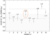 |
Fig. 1. X-ray count rate in the [0.3–4] keV band of light jet models, named in the horizontal axis as described in Table 1. In the vertical axis we plot the median count rate in every case (represented with a diamond). The lower and upper error bars indicate the 15th and 85th percentile, respectively. The dashed lines indicate the interval of the count rate observed for HH 154. The orange circle indicates the reference case. The shadowed part corresponds to the scale of Fig. 6, which summarizes the heavy jet models described in the next subsection. |
Summary of the initial physical parameters characterizing the different models.
3.1.1. Reference case
In Fig. 2 we present the 2D spatial distributions of temperature, density, and count rate of model LJ5 (see Table 1) in three different moments. The complete temporal evolution is available as an online movie (Movie 1). The animation starts when the pulsed component is introduced, formed from a train of blobs with a blob-to-jet particle number density ratio χb = 3 (see Table 1), and covers the evolution of the pulsed jet for approximately 50 years. The upper panels in Fig. 2 show 2D maps of temperature (left half-panels) and density (right half-panels), both in logarithmic scale. The lower panels show the 2D spatial distribution of X-ray count rate in the [0.3–4] keV band with resolution of 0.5″(Chandra native resolution), derived from the simulations as described in Sect. 2.3.
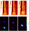 |
Fig. 2. Model LJ5 at different evolution times: t ≈ 72 yr (left panels), t ≈ 74 yr (middle panels), and t ≈ 100 yr (right panels). Upper panels: two-dimensional maps of temperature (left half-panels), and density (right half-panels) distributions. Lower panels: maps of X-ray count rate in the [0.3–4] keV band with macropixel resolution of 0.5″. |
The left panels in Fig. 2 show the stationary shock when the first blob is arriving at t ≈ 72 yr, for model LJ5. The shock forms when the flow expands and is collimated by the ambient magnetic field heating the plasma to temperatures of a few million degrees (see Ustamujic et al. 2016 for a detailed description). The plasma density and temperature reach respective maximum values of ~6 × 103 cm−3 and ~7 × 10⁶ K at the shock. The shock temperature, calculated as the density-weighted average temperature considering only the cells with T ≥ 106, is ~3 × 10⁶ K. The pre-shock density is ~500 cm−3, one order of magnitude lower than the ambient medium density, namely ~5000 cm−3. The count rate map in the [0.3–4] keV band, calculated as described in Sect. 2.3, shows that the X-ray emission comes mainly from the shock diamond (see lower left panel in Fig. 2). The X-ray total shock luminosity, LX, derived in the [0.3–4] keV band is ~5 × 1029 erg s−1. In Fig. 3 (upper panel) we plot the pressure profiles along the jet axis at t ≈ 72 yr. Close to the jet axis the model evolution is dominated by the jet plasma pressure (P, represented in green) over the magnetic pressure (Pm, represented in blue), where the plasma β (defined as the ratio of the plasma pressure to the magnetic pressure) is higher than 1 (β > 1). In black, we plot the ram pressure defined as Pr = ρ · u2, where ρ and u are the density and velocity, respectively. Finally, we represent in red the dynamic pressure, H = P + Pr, almost constant along the profile due to the stability and quasi-stationarity of the model. The central panels in Fig. 2 show the jet at t ≈ 74 yr, when the first blob has just passed through the shock and the second one is arriving. The shocked plasma density and temperature maintain mostly the same values as before: maximum values of ~6 × 103 cm−3 and ~7 × 10⁶ K, and a density-weighted average temperature of ~3 × 10⁶ K. The X-ray source is perturbed and moved by the blob (see lower middle panel in Fig. 2). The X-ray total shock luminosity, LX, derived in the [0.3–4] keV band is ~6×1029 erg s−1. In Fig. 3 (middle panel) we observe the perturbation effect in the pressure profiles along the jet axis at t ≈ 74 yr, when the blob has just passed, affecting the shock stability slightly. The right panels in Fig. 2 show the jet at t ≈ 100 yr, after a train of blobs has passed through the shock. The shocked plasma maximum values for density and temperature are ~3 × 103 cm−3 and ~1 × 10⁷ K, respectively, and the density-weighted average temperature is ~3 × 10⁶ K. The X-ray emission in the [0.3–4] keV band is enhanced by the perturbations and the source is located at the base of the jet (see lower right panel in Fig. 2). The X-ray total shock luminosity, LX, derived in the [0.3–4] keV band is ~7×1029 erg s−1. In Fig. 3 (lower panel) we observe the pressure profiles along the jet axis at t ≈ 100 yr, completely perturbed by the train of blobs.
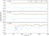 |
Fig. 3. Pressure profiles at r = 0 for model LJ5 at t ≈ 72 yr (upper panel), t ≈ 74 yr (middle panel), and t ≈ 100 yr (lower panel). We plot ram pressure in black, magnetic pressure in blue, thermal pressure in green, and dynamic pressure in red. |
3.1.2. Variability
In order to investigate the stationarity of the different pulsed jet models, we study the variations of the physical quantities (shock temperature, density of the X-ray emitting component, X-ray luminosity, etc.) and of the spatial distribution of the count rate during the evolution of the model. We derive the total count rate in the [0.3–4] keV band, calculated as described in Sect. 2.3, and integrated in the whole domain to obtain the total value. In Fig. 4 we show one value of count rate with Poisson error bars per year, omitting the first five values corresponding to the initial transient of the pulsed jet. The dashed lines correspond to the interval [0.57,1.01], which contains the count rate values derived from observations by Bonito et al. (2011). We note that the values derived from the model are compatible with the observations during all the evolution. The temporal evolution of the spatial distribution of the count rate for model LJ5, as would be seen by the Chandra/ACIS instrument, is shown in the right panel of the first movie (Movie 1). We observe two different components emitting in X-rays during all the animation: one quasi-stationary at the base of the jet, and another fainter in the direction of propagation of the jet. In order to understand the trend of the X-ray emission we integrate in time and along the jet radius, omitting the frames corresponding to the initial transient. In this way, we derive the count rate profile along the jet axis (see Fig. 5). We find that most of the X-ray emission clearly comes from the source close to the base of the jet. We also discern a fainter X-ray source further away, as observed in HH 154 by Bonito et al. (2011).
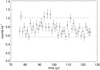 |
Fig. 4. X-ray count rate in the [0.3–4] keV band with error bars for model LJ5. We plot one point every year. The dashed lines indicate the interval of the count rate observed for HH 154. |
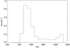 |
Fig. 5. X-ray count rate profile along the jet axis calculated integrating the 2D maps of the LJ5 model evolution in time and along the jet radius r. |
3.1.3. Comparison with the other models
We compare different models for the light jet scenario in order to investigate the effect of perturbations in the stationarity of the shock. The explored parameters are listed in Table 1, namely jet temperature and density; blob density, velocity, and radius; the rotation; and the mass loss rate. The jet temperature and density, and the possible rotation affect both continuous and pulsed components and determine the physical parameters of the shock (see Ustamujic et al. 2016). They are selected according to the observations of HH 154 (Favata et al. 2002, 2006; Bonito et al. 2011). The parameters of the blob (density, velocity, and radius) are those that determine the strength of the perturbation. The mass loss rate is calculated as explained in Sect. 2.2 and gives information about the intensity of the perturbations introduced through the amplitude of its variation. The values obtained for all the models are of the order of ~10−8M⊙yr−1, in good agreement with typical outflow rates found in pre-main sequence stars (Cabrit et al. 2007; Podio et al. 2011). In our reference model (LJ5) the jet initial temperature and density are Tj = 3 × 10⁶ K and nj = 104 cm−3 respectively. In cases with higher values of jet temperature and density, namely LJ9 and LJ10, the shock is stronger and the count rate is higher (see Fig. 1). In model LJ3, with the same parameters as LJ5 but without rotation, the count rate is lower because the shock is weaker, as was already predicted by Ustamujic et al. (2016). We do not observe a significant effect on the stability of the shock due to the rotation. The parameters that directly affect the stationarity of the emitting shock are those that define the blobs perturbing it. The parameters defining the blob density, velocity, and radius in models LJ5 (reference case) and LJ3 are χb = 3, υb = 500 km s−1, and Rb = 1, respectively (see Table 1). When the blob density is lower (e.g. in LJ6, χb = 1.5), the median count rate and the perturbations are lower, whereas for a higher blob density (e.g. in LJ8, χb = 10), they are higher than in LJ3. When the radius is lower (e.g. LJ4 with respect to LJ3, and LJ7 with respect to LJ6) the median count rate and the perturbations are lower. This effect is more evident in LJ4 because the perturbation is stronger. Finally, when we compare models with random velocity to those with constant velocity (e.g. LJ1 with respect to LJ3, and LJ2 with respect to LJ6), we do not observe a significant change.
In summary, we can affirm that the perturbations are compatible with the available observations of HH 154. The jet forms a quasi-stationary X-ray emitting shock at the base of the jet and the perturbations arriving from the protostellar source as a train of blobs contribute to the emission enhancing the total count rate. The variations registered in the count rate are comparable with those observed for perturbations in the following ranges: density increase of a maximum of one order of magnitude, velocity fluctuation of 50%, and radius with values from 1/3 to 1 jet radius are compatible. The maximum change in the mass loss rate derived is approximately one order of magnitude in model LJ8, for which the total count rate calculated variations are at the limit of the values observed by Bonito et al. (2011).
3.2. Heavy jet: the case of the jet associated to DG Tau
Most of the models explored in the heavy jet scenario reproduce well the case of DG Tau. In Fig. 6 we summarize the results for the count rate for the different models described in Table 1.
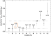 |
Fig. 6. X-ray count rate in the [0.5–1] keV band of heavy jet models, named in the horizontal axis as described in Table 1. In the vertical axis we plot the median count rate in every case (represented with a diamond). The lower and upper error bars represent the 15th and 85th percentile respectively. The dashed lines indicate the interval of the count rate observed for DG Tau. The orange circle indicates the reference case. |
For every model we derive the X-ray count rate in the [0.5–1] keV band during the evolution (one value per year) as decribed in Sect. 2.3, and then we calculate the median and the 15% and 85% percentiles of all the values in each case. The dashed lines indicate the interval containing the X-ray count rate values (considering errors) derived from observations by Güdel et al. (2005, 2008, 2011), namely 0.20 ± 0.08, 0.18 ± 0.06 and 0.11 ± 0.02 counts ks−1. As in the light jet scenario, this representation allows us to compare the different models between them and with the values observed. The models that best fit with the DG Tau observations are HJ3, HJ7, HJ8, and HJ9 (see Fig. 6). We assume HJ3 (marked with an orange circle in Fig. 6) as our reference case and we describe it in detail in the next section.
3.2.1. Reference case
As Fig. 2, Fig. 7 presents the 2D spatial distributions of temperature, density, and count rate for model HJ3 (see Table 1) in three different moments. The complete temporal evolution is available as an online movie (Movie 2). The animation starts when the pulsed component is introduced, formed from a train of blobs with blob-to-jet particle number density ratio χb = 1.5 (see Table 1), and covers the evolution of the pulsed jet for approximately 50 years.
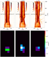 |
Fig. 7. Model HJ3 at different evolution times: t ≈ 42 yr (left panels), t ≈ 44 yr (middle panels), and t ≈ 70 yr (right panels). Upper panels: two-dimensional distribution maps of temperature (left half-panels) and density (right half-panels). Lower panels: maps of X-ray count rate in the [0.5–1] keV band with macropixel resolution of 0.5″. |
The left panels in Fig. 7 show the stationary shock when the first blob is arriving at t ≈ 42 yr, for model HJ3. The stationary shock forms in the same way as described in Sect. 3.1 for the light jet scenario (see also Ustamujic et al. 2016). The plasma density and temperature reach respective maximum values of ~1 × 104 cm−3 and ~5 × 10⁶ K at the shock. The shock temperature, calculated as the density-weighted average temperature considering only the cells with T 106, is ~2 × 10⁶ K. The pre-shock density is ~1000 cm−3, one order of magnitude higher than the ambient medium density, namely ~100 cm−3. The count rate map in the [0.5–1] keV band, calculated as described in Sect. 2.3, shows that the X-ray emission comes mainly from the shock diamond (see lower left panel in Fig. 7). The X-ray total shock luminosity, LX, derived in the [0.5–1] keV band is ~2 × 1029 erg s−1. In Fig. 8 (upper panel) we plot the pressure profiles along the jet axis at t ≈ 42 yr. As in the light jet scenario, the model evolution close to the jet axis is dominated by the jet plasma pressure (P, represented in green) over the magnetic pressure (Pm, represented in blue), where β > 1. In this case the plasma pressure, and thus β, is lower compared with the case studied in the light jet scenario (see Fig. 3). We plot the ram pressure Pr (black) and the dynamic pressure H (red), which is almost constant along the profile due to the stability and quasistationarity of the model. The central panels in Fig. 7 show the jet at t ≈ 44 yr, when the first blob has just passed through the shock and the second one is arriving. The shocked plasma density and temperature are higher after the perturbation: maximum values of ~6 × 104 cm−3 and ~1 × 10⁷ K, and density-weighted average temperature of ~3 × 10⁶ K. The X-ray source is perturbed, but it is still located at the base of the jet (see lower middle panel in Fig. 7). The X-ray total shock luminosity LX in the [0.5–1] keV band is ~2 × 1029 erg s−1. In Fig. 8 (middle panel) we observe the perturbation effect in the pressure profiles along the jet axis at t ≈ 44 yr when the blob has just passed, which strongly affects the profiles’ stability. The right panels in Fig. 7 show the jet at t ≈ 70 yr, after a train of blobs has passed through the shock. The shocked plasma maximum values for density and temperature are ~5 × 104 cm−3 and ~1 × 10⁷ K, respectively, and the density-weighted average temperature is ~2 × 10⁶ K. The X-ray source is located at the base of the jet (see lower right panel in Fig. 7), with a total shock luminosity LX similar to the values derived before, namely ~2 × 1029 erg s−1. In Fig. 8 (lower panel) we observe the pressure profiles along the jet axis at t ≈ 70 yr, completely perturbed by the train of blobs.
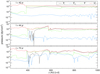 |
Fig. 8. Pressure profiles at r = 0 for model HJ3 at t ≈ 42 yr (upper panel), t ≈ 44 yr (middle panel), and t ≈ 70 yr (lower panel). We plot ram pressure in black, magnetic pressure in blue, thermal pressure in green, and dynamic pressure in red. |
3.2.2. Variability
As in Sect. 3.1.2 we investigate the stationarity of the different pulsed jet models by studying the variations of the physical quantities and of the spatial distribution of the count rate during the evolution. We derive the total count rate in the [0.5–1] keV band, calculated as described in Sect. 2.3 and integrated in the whole domain to obtain the total value. In Fig. 9 we show one value of count rate with Poisson error bars per year, omitting the first five values corresponding to the initial transient of the pulsed jet observed at the beginning of the animation (Movie 2). The dashed lines correspond to the interval [0.09,0.28], which contains the count rate values derived from observations by Güdel et al. (2005, 2008, 2011). We note that the values derived from the model are in good agreement with the observations during the whole evolution for the parameters explored here5. The temporal evolution of the spatial distribution of the count rate for model HJ3, as would be seen by the Chandra/ACIS instrument, is shown in the right panel of the second movie (Movie 2). In this case, we observe one single component emitting in X-rays at the base of the jet throughout almost the whole animation. In order to understand the trend, in the same way as described in Sect. 3.1, we derive the count rate profile along the jet axis (see Fig. 10). We find that most of the X-ray emission comes from one single source close to the base of the jet.
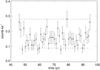 |
Fig. 9. X-ray count rate in the [0.5–1] keV band with error bars for model HJ3. We plot one point every year. The dashed lines indicate the interval of the count rate observed for the DG Tau jet. A different scale is used for the y-axis with respect to Fig. 6. |
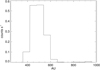 |
Fig. 10. X-ray count rate profile along the jet axis calculated integrating the 2D maps of the HJ3 model evolution in time and along the jet radius r. |
3.2.3. Comparison with the other models
We compare different models for the heavy jet scenario in order to investigate the effect of perturbations in the stationarity of the shock. The explored parameters, which describe the jet and the blobs, are listed in Table 1. The jet temperature and density and the possible rotation determine the physical parameters of the shock (see Ustamujic et al. 2016). They are selected according to the observations of DG Tau (Güdel et al. 2005, 2008). The parameters of the blob (density, velocity, and radius) and the mass loss rate, calculated as explained in Sect. 2.2, give information about the intensity of the perturbations introduced. In our reference model (HJ3) the jet initial temperature and density are Tj = 106 K and nj = 104 cm−3, respectively. In cases with higher values of jet temperature and density, namely models HJ9–HJ12, the shock is stronger and the count rate is higher (see Fig. 6). As in the light jet scenario, for the models including jet rotation, namely HJ2, HJ3, and HJ6, the count rate is higher because the shock is stronger (as predicted by Ustamujic et al. 2016). This trend is clear when we compare same models with and without jet rotation, e.g. HJ6 and HJ4 (see Fig. 6). Again we do not observe a significant effect on the stability of the shock due to the rotation. The parameters that define blob density and radius in model HJ3 (reference case) are χb = 1.5 and Rb = 1/3, respectively, while the velocity υb varies randomly from 300 to 700 km s−1 (see Table 1). The random velocity makes the perturbation stronger due to the higher variations in the ram pressure, which lowers the count rate slightly, although the effect in the studied cases is very faint and not significant (see models HJ1 and HJ4 in Fig. 6). When the blob radius is higher (e.g. HJ2 with respect to HJ3, and HJ4 with respect to HJ5) the shock is slightly affected, which lowers the median count rate and enhances the fluctuations. When the blob density is increased, we find different effects depending on the part of the domain being considered. In low count rate models an increase in the blob density perturbs the shock and lowers the count rate (e.g. HJ5 with respect to HJ8), while in high count rate models the median count rate increases, which contributes to the emission (e.g. HJ12 with respect to HJ10), as in the light jet scenario. We investigate the difference between the models through the pressure profiles (see Figs. 3 and 8). In all the cases the jet is dominated by the plasma pressure over the magnetic pressure, i.e. β > 1, but in cases with a low count rate we find a more instable regime because the β parameter is closer to 1 in some moments of the simulation. This means that the perturbations affect models with high and low count rates in different ways. Model HJ9 is situated at the limit of the two different regimes described, and when higher density blobs are introduced (model HJ11), the median count rate remains almost constant.
In summary, we can affirm that the perturbations are compatible with the available observations of DG Tau in most of the cases explored. The jet forms a quasi-stationary X-ray emitting shock at the base which is more likely affected by perturbations arriving from the stellar source as a train of blobs. In this case, the X-ray emitting shock is more perturbed than that of HH 154 due to the low count rate observed for the DG Tau jet. Strong perturbations can almost erase the X-ray emission from a shock in models with low count rate, while in models with higher count rate values the X-ray emission is enhanced, in a similar way to the light jet scenario of HH 154. The variations registered in the count rate are comparable with those observed for perturbations in the following ranges: density increase of a maximum of three times the previous value, velocity fluctuation of 50%, and radius with values from 1/3 to 1 jet radius are compatible. The mass loss rate values obtained for all the models are Ṁj ∼ 10−8 M⊙yr−1, in good agreement with typical outflow rates found in pre-main sequence stars (Cabrit et al. 2007; Podio et al. 2011). The maximum change in Ṁj is approximately a half order of magnitude in model HJ1, for which the total count rate is very low; it is not compatible with the values observed for DG Tau by Güdel et al. (2005, 2008, 2011).
4. Discussion
In a previous study (Ustamujic et al. 2016), we showed that a continuously driven stellar jet forms a stationary X-ray emitting shock at the base with physical parameters in good agreement with observations. The aim of this work is to investigate whether the quasi-stationary shocks formed are compatible with the perturbations expected in YSO jets through simulations of a pulsed flow, and derive the physical parameters that can give rise to X-ray emission consistent with observations of jets in pre-main sequence stars. To this end we developed a MHD 2.5D model that describes the propagation of a supersonic stellar jet in a initially homogeneous magnetized medium taking into account the effect of the radiative cooling. The jet is described by two components: a continuously driven component that forms a quasistationary shock at the base of the jet, and a pulsed component formed of blobs that introduce perturbations into the jet influencing the shock. In order to compare the model results with observations we synthesized the count rate from the simulations, considering both its total integrated value and its spatial distribution.
Previous MHD models of protostellar jets were more oriented towards studying the dynamical aspects and the evolution of the jet rather than the X-ray emission produced. Here we show the feasibility of our MHD model: a supersonic stellar jet collimated by the ambient magnetic field leading to X-ray emission from the shock formed at the base, consistent with the observations. We obtained shock temperatures of ~106 K and luminosities of L X ≈ 1029 erg s−1, in good agreement with the X-ray results of other authors (Pravdo et al. 2001; Favata et al. 2002; Bally et al. 2003; Pravdo & Tsuboi 2005; Güdel et al. 2008; Schneider et al. 2011; Skinner et al. 2011; López-Santiago et al. 2013, 2015).
As YSO jets are intrinsically dynamic objects which evolve on timescales of a few years, they are ideal laboratories for variability studies. We selected HH 154 and DG Tau as specific targets for our study because available observations suggest the presence of stationary X-ray emitting sources close to the base associated with the jet (HH 154, Favata et al. 2006; DG Tau, Güdel et al. 2005). Chandra X-ray observations collected in different epochs for HH 154 (in 2001, Bally et al. 2003; in 2005, Favata et al. 2006; in 2009, Schneider et al. 2011) and for DG Tau’s jet (in 2004, 2006, and 2010, Güdel et al. 2005, 2008, 2011), provided a time base of eight and six years, respectively, to analyse the variability of the source. They are, as far as we know, the only YSO jets with available multi-epoch X-ray observations.
4.1. The case of HH 154
In the light jet scenario (see Sect. 3.1) we described a jet that is less dense than the ambient medium, for example the jet related to HH 154 which originates from the deeply embedded binary Class 0/I protostar IRS 5 in the L1551 star-forming region (Rodríguez et al. 1998).
Figure 11 shows the count rate of the X-ray source associated with HH 154 in the [0.3–4] keV band. We compare the data set observed by Chandra/ACIS in 2005 and analysed by Bonito et al. (2011) (left panel), with the synthetic map derived from model LJ5 (reference case for the light jet presented in Sect. 3.1) at t = 100 yr, and convolved with the specific PSF created at the proper energy (right panel). The images are rebinned to match a pixel size of 0.25″, and then a Gaussian smoothing with kernel of width 0.5″ was applied. Bonito et al. (2011) analysed Chandra multi-epoch X-ray observations of HH 154 (in 2001, Bally et al. 2003; in 2005, Favata et al. 2006; in 2009, Schneider et al. 2011) and proposed the scenario of a nozzle creating the standing shock in the presence of a pulsed jet, as described in Bonito et al. (2010b), which may account for the elongated component as a newly formed knot propagating away from the diamond shock. Here we propose an alternative possible interpretation: the bright stationary X-ray source observed in the data might be associated with the main stationary shock formed at the base of the jet, whereas the faint, elongated, and more variable component could be the result of perturbations of the main shock. As discussed by Bonito et al. (2011), the X-ray source associated with HH 154 unambiguously arises from the jet and cannot be of stellar origin.
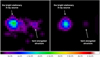 |
Fig. 11. Smoothed X-ray count rate maps in the [0.3–4] keV band for HH 154 with a pixel size of 0.25″. Left: 2005 data set resampled using the EDSER technique, as in Bonito et al. (2011). Right: Synthetic image of the base of the jet as derived from model LJ5 at t = 100 yr (see lower right panel in Fig. 2), rebinned to match the same pixel size and convolved with the proper PSF. The angular size of each panel is ≈7″ × 7″. In each panel north is up and east is left. Gaussian smoothing was applied on the images with kernel of width 0.5″. |
4.2. The case of the jet associated to DG Tau
In the heavy jet scenario (see Sect. 3.2) we described a jet that is denser than the ambient medium, for example the jet associated with DG Tau which originates from a more evolved Class II diskbearing source (CTTS) (see Eislöffel & Mundt 1998).
In Fig. 12 we show the count rate of the X-ray source associated with DG Tau in the [0.5–1] keV band, in logarithmic scale. In the left panel we plot the merged data set observed by Chandra/ACIS in 2010 (see Appendix A for a detailed description of the data analysis we performed) with a pixel size of 0.25″ and Gaussian smoothing with kernel of width 0.5″. In this case the angular size of each panel is ≈ 14″ × 14″ (we note that the scale is different from that in Fig. 11, which corresponds only to one quadrant of this image). The observation shows the star marked with a cross inside the central unresolved source, and a bipolar jet. In this image the SW jet marked with a box is clearly visible, while the counter-jet (observed earlier by Güdel et al. 2005, 2008) is hardly visible. The central unresolved source contains two unrelated spectral components subject to different hydrogen absorption column densities (Güdel et al. 2011): the hard component is associated with the stellar corona or magnetosphere, while the soft component is associated with X-ray emission from the base of the jet produced either by internal shocks or by magnetic heating (Güdel et al. 2008). Recently, Takasao et al. (2017) have presented a theoretical model applied to DG Tau in which the disk atmosphere is magnetically heated forming a hot corona emitting in soft X-rays. However, in these data it is still unclear, due to the contamination from the star, which part of the soft component of the X-ray emission is produced by the jet. For this reason, we compare our jet results with the SW jet marked with a box in the left panel of Fig. 12. On the right we plot the synthetic map of the modelled region derived from model HJ3 (reference case for the heavy jet presented in Sect. 3.2) at t = 70 yr, and convolved with the specific PSF created at the proper energy. Again, the image is rebinned to match a pixel size of 0.25″ and then smoothed with a Gaussian kernel of width 0.5″. In this case the synthesized source consists of one unique component, while in the case of HH 154 (see Fig. 11) we were able to observe cleary two different components. The size and morphology of the synthesized source is comparable with the SW jet observations.
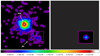 |
Fig. 12. Smoothed X-ray count rate maps in the [0.5–1] keV band for DG Tau in logarithmic scale and with a pixel size of 0.25″. Left: 2010 data set resampled using the EDSER technique, as explained in Appendix A. We marked the position of the star with a cross and the SW jet with a box. Right: Synthetic image of the base of the jet as derived from model HJ3 at t = 70 yr (see lower right panel in Fig. 7), rebinned to match the same pixel size and convolved with the specific PSF. The modelled region is marked with a box corresponding to the SW jet. The angular size of each panel is ≈14″×14″ (a different scale to that used in Fig. 11). In each panel north is up and east is left. Gaussian smoothing was applied on the images with kernel of width 0.5″. |
5. Summary and conclusions
We investigated the effect of perturbations in X-ray emitting stationary shocks in stellar jets through numerical MHD simulations. We applied our model to the X-ray jets of HH 154 and DG Tau, two widely studied objects at different stages of evolution. This allowed us to explore the similarities and differences of YSOs at distinct stages of evolution through the study of the X-ray emission and jets which are present in objects from Class 0 to II. We have also performed a wide exploration of a broad region of the parameter space that describes the model (see Table 1). These results therefore allow us to study and diagnose the physical properties of YSO jets over a broader range of physical conditions than those defined by HH 154 and DG Tau. Our findings lead to several conclusions, that we list in the following for the two different scenario studied (LJ and HJ).
LJ scenario (HH 154):
We find that perturbations arriving to the shock as a train of blobs contribute to the X-ray emission enhancing the total count rate.
Perturbations characterized by a density increase up to one order of magnitude, velocity fluctuations not larger than 50%, and size with values from 1/3 to 1 of the initial jet radius produce variability in the X-ray source compatible with that observed in HH 154 (Bonito et al. 2011).
The perturbations explored lead to maximum variations of approximately one order of magnitude in the mass loss rate derived from the simulations.
HJ scenario (DG Tau):
The stability of the shock diamond is affected by the jet perturbations more easily in the HJ than in the LJ scenario. This is mainly due to the fact that the shock in the HJ scenario is fainter and with a lower total count rate than in the LJ scenario (see Fig. 6). In addition, models with a lower median count rate (e.g. HJ1–HJ8) are more affected by the perturbations than models with higher median count rate (e.g. HJ9–HJ12). In the latter models, the perturbations enhance the X-ray emission as in the light jet scenario.
Perturbations characterized by a density increase up to three times the initial jet value, velocity fluctuations not larger than 50%, and size with values from 1/3 to 1 initial jet radius produce variability of X-ray source compatible with that observed in the SW jet of DG Tau (Güdel et al. 2008, 2011).
The perturbations explored lead to maximum variations of ~1–4 · Ṁj in the mass loss rate derived from the simulations (see Table 1), corresponding to fainter perturbations than those presented in the LJ scenario.
In both the scenarios explored, although the physical conditions are very different, the plasma is collimated by the magnetic field forming a quasi-stationary shock at the base of the jet which, under certain conditions, emits in X-rays even when perturbations are present. The results presented here may provide us with a better understanding of the evolution and the different mechanisms observed in young stars at different stages of evolution. Although the precise mechanisms are still under debate, it is widely believed that the strongly dynamic and energetic phenomena due to star-disk interaction produce variations in the physical parameters of the jet. The study of the variability observed in pre-main sequence stars may give some insight into the phenomena that occur due to the star disk interaction, also related to the still debated jet collimation and acceleration mechanisms. Finally, the comparison of our MHD model results with the X-ray observations could provide a fundamental tool for investigating the stellar jet dynamics and the high-energy phenomena, also important for a better understanding of planet formation.
Movies
Movie 1 Access Supplementary Material
Movie 2 Access Supplementary Material
Acknowledgments
S.U. acknowledges the hospitality of the INAF Osservatorio Astronomico di Palermo, where part of the present work was carried out using the HPC facility (SCAN). PLUTO is being developed at the Turin Astronomical Observatory in collaboration with the Department of General Physics of the Turin University. This research has made use of data obtained from the Chandra Data Archive (published previously in the cited articles), and software provided by the Chandra X-ray Center (CXC) in the application package CIAO. This work was supported by grant BES-2012-061750 from the Spanish Government under research project AYA2011-29754-C03-01, and by the Ministry of Economy and Competitivity of Spain under grant numbers ESP2014-54243-R and ESP2015-68908-R. The research leading to these results has also received funding from the European Union’s Horizon 2020 Programme under the AHEAD project (grant agreement n. 654215). R. B. acknowledges financial support from INAF under PRIN2013 Programme ‘Disks, jets and the dawn of planets’. We would like to thank Dr. Francesco Damiani for helpful discussions. Finally, we thank the referee for the useful comments and suggestions.
We verified the assumptions used in this paper as described in Bonito et al. (2007).
See Fig. 3 in Ustamujic et al. (2016).
See Bonito et al. (2008) and Fig. 4 in Bonito et al. (2010b).
See Ustamujic et al. (2016) for more details about the formation of X-ray emitting shocks at magnetized protostellar jets.
References
- Albertazzi, B., Ciardi, A., Nakatsutsumi, M., et al. 2014, Science, 346, 325 [NASA ADS] [CrossRef] [Google Scholar]
- Anders, E., & Grevesse, N. 1989, Geochim. Cosmochim. Acta, 53, 197 [Google Scholar]
- Andre, P., & Montmerle, T. 1994, ApJ, 420, 837 [NASA ADS] [CrossRef] [Google Scholar]
- Bacciotti, F., Ray, T. P., Mundt, R., Eislöffel, J., & Solf, J. 2002, ApJ, 576, 222 [NASA ADS] [CrossRef] [Google Scholar]
- Bally, J., Feigelson, E., & Reipurth, B. 2003, ApJ, 584, 843 [NASA ADS] [CrossRef] [Google Scholar]
- Balsara, D. S., & Spicer, D. S. 1999, J. Comput. Phys., 149, 270 [Google Scholar]
- Bodo, G., Massaglia, S., Ferrari, A., & Trussoni, E. 1994, A&A, 283, 655 [NASA ADS] [Google Scholar]
- Bonito, R., Orlando, S., Peres, G., Favata, F., & Rosner, R. 2004, A&A, 424, L1 [NASA ADS] [CrossRef] [EDP Sciences] [Google Scholar]
- Bonito, R., Orlando, S., Peres, G., Favata, F., & Rosner, R. 2007, A&A, 462, 645 [NASA ADS] [CrossRef] [EDP Sciences] [Google Scholar]
- Bonito, R., Fridlund, C. V. M., Favata, F., et al. 2008, A&A, 484, 389 [NASA ADS] [CrossRef] [EDP Sciences] [Google Scholar]
- Bonito, R., Orlando, S., Miceli, M., et al. 2010a, A&A, 517, A68 [NASA ADS] [CrossRef] [EDP Sciences] [Google Scholar]
- Bonito, R., Orlando, S., Peres, G., et al. 2010b, A&A, 511, A42 [NASA ADS] [CrossRef] [EDP Sciences] [Google Scholar]
- Bonito, R., Orlando, S., Miceli, M., et al. 2011, ApJ, 737, 54 [CrossRef] [Google Scholar]
- Cabrit, S. 2007, in Lecture Notes in Physics, ed. J. Ferreira, C. Dougados, & E. Whelan, (Berlin: Springer Verlag), 723, 21 [Google Scholar]
- Cabrit, S., Edwards, S., Strom, S. E., & Strom, K. M. 1990, ApJ, 354, 687 [NASA ADS] [CrossRef] [Google Scholar]
- Cabrit, S., Codella, C., Gueth, F., et al. 2007, A&A, 468, L29 [NASA ADS] [CrossRef] [EDP Sciences] [Google Scholar]
- Ciardi, A., Lebedev, S. V., Frank, A., et al. 2009, ApJ, 691, L147 [NASA ADS] [CrossRef] [Google Scholar]
- Coffey, D., Bacciotti, F., Ray, T. P., Eislöffel, J., & Woitas, J. 2007, ApJ, 663, 350 [NASA ADS] [CrossRef] [Google Scholar]
- de Colle, F., & Raga, A. C. 2006, A&A, 449, 1061 [NASA ADS] [CrossRef] [EDP Sciences] [Google Scholar]
- Eislöffel, J., & Mundt, R. 1998, AJ, 115, 1554 [NASA ADS] [CrossRef] [Google Scholar]
- Favata, F., Fridlund, C. V. M., Micela, G., Sciortino, S., & Kaas, A. A. 2002, A&A, 386, 204 [NASA ADS] [CrossRef] [EDP Sciences] [Google Scholar]
- Favata, F., Bonito, R., Micela, G., et al. 2006, A&A, 450, L17 [NASA ADS] [CrossRef] [EDP Sciences] [Google Scholar]
- Feigelson, E. D., & Montmerle, T. 1999, ARA&A, 37, 363 [NASA ADS] [CrossRef] [Google Scholar]
- Ferreira, J., Dougados, C., & Cabrit, S. 2006, A&A, 453, 785 [NASA ADS] [CrossRef] [EDP Sciences] [Google Scholar]
- Frank, A., Ray, T. P., Cabrit, S., et al. 2014, Protostars and Planets VI (Tucson: University of Arizona Press), 451[1pc] [Google Scholar]
- Fridlund, C. V. M., Liseau, R., & Gullbring, E. 1998, A&A, 330, 327 [NASA ADS] [Google Scholar]
- Güdel, M., Skinner, S. L., Briggs, K. R., et al. 2005, ApJ, 626, L53 [NASA ADS] [CrossRef] [Google Scholar]
- Güdel, M., Skinner, S. L., Audard, M., Briggs, K. R., & Cabrit, S. 2008, A&A, 478, 797 [NASA ADS] [CrossRef] [EDP Sciences] [Google Scholar]
- Güdel, M., Audard, M., Bacciotti, F., et al. 2011, in 16th Cambridge Workshop on Cool Stars, Stellar Systems, and the Sun, eds. C. Johns-Krull, M. K. Browning, & A. A. West, ASP Conf. Ser., 448, 617 [NASA ADS] [Google Scholar]
- Hartigan, P., Edwards, S., & Ghandour, L. 1995, ApJ, 452, 736 [NASA ADS] [CrossRef] [Google Scholar]
- Kashyap, V., & Drake, J. J. 2000, Bull. Astron. Soc. India, 28, 475 [NASA ADS] [EDP Sciences] [Google Scholar]
- Lada, C. J. 1987, in Star Forming Regions, eds. M. Peimbert, & J. Jugaku, IAU Symp., 115, 1 [NASA ADS] [CrossRef] [Google Scholar]
- Li, J., Kastner, J. H., Prigozhin, G. Y., et al. 2004, ApJ, 610, 1204 [NASA ADS] [CrossRef] [Google Scholar]
- López-Santiago, J., Peri, C. S., Bonito, R., et al. 2013, ApJ, 776, L22 [Google Scholar]
- López-Santiago, J., Bonito, R., Orellana, M., et al. 2015, ApJ, 806, 53 [NASA ADS] [CrossRef] [Google Scholar]
- Masciadri, E., Velázquez, P. F., Raga, A. C., Cantó, J., & Noriega-Crespo, A. 2002, ApJ, 573, 260 [NASA ADS] [CrossRef] [Google Scholar]
- Mignone, A., Bodo, G., Massaglia, S., et al. 2007, ApJS, 170, 228 [Google Scholar]
- Orlando, S., Reale, F., Peres, G., & Mignone, A. 2011, MNRAS, 415, 3380 [NASA ADS] [CrossRef] [Google Scholar]
- Podio, L., Eislöffel, J., Melnikov, S., Hodapp, K. W., & Bacciotti, F. 2011, A&A, 527, A13 [NASA ADS] [CrossRef] [EDP Sciences] [Google Scholar]
- Pravdo, S. H., & Tsuboi, Y. 2005, ApJ, 626, 272 [NASA ADS] [CrossRef] [Google Scholar]
- Pravdo, S. H., Feigelson, E. D., Garmire, G., et al. 2001, Nature, 413, 708 [NASA ADS] [CrossRef] [PubMed] [Google Scholar]
- Pravdo, S. H., Tsuboi, Y., & Maeda, Y. 2004, ApJ, 605, 259 [NASA ADS] [CrossRef] [Google Scholar]
- Pudritz, R. E., & Norman, C. A. 1983, ApJ, 274, 677 [NASA ADS] [CrossRef] [Google Scholar]
- Pudritz, R. E., & Norman, C. A. 1986, ApJ, 301, 571 [NASA ADS] [CrossRef] [Google Scholar]
- Pudritz, R. E., Ouyed, R., Fendt, C., & Brandenburg, A. 2007, Protostars and Planets V (Tucson: University of Arizona Press), 277 [Google Scholar]
- Raga, A., & Noriega-Crespo, A. 1998, AJ, 116, 2943 [NASA ADS] [CrossRef] [Google Scholar]
- Raga, A. C., Binette, L., Canto, J., & Calvet, N. 1990, ApJ, 364, 601 [NASA ADS] [CrossRef] [Google Scholar]
- Raga, A., Cabrit, S., Dougados, C., & Lavalley, C. 2001, A&A, 367, 959 [NASA ADS] [CrossRef] [EDP Sciences] [Google Scholar]
- Raga, A. C., Riera, A., Masciadri, E., et al. 2004, AJ, 127, 1081 [NASA ADS] [CrossRef] [Google Scholar]
- Raga, A. C., de Colle, F., Kajdič, P., Esquivel, A., & Cantó, J. 2007, A&A, 465, 879 [NASA ADS] [CrossRef] [EDP Sciences] [Google Scholar]
- Raga, A. C., Riera, A., & González-Gómez, D. I. 2010, A&A, 517, A20 [NASA ADS] [CrossRef] [EDP Sciences] [Google Scholar]
- Reipurth, B., & Bally, J. 2001, ARA&A, 39, 403 [NASA ADS] [CrossRef] [Google Scholar]
- Rodríguez, L. F., D’Alessio, P., Wilner, D. J., et al. 1998, Nature, 395, 355 [NASA ADS] [CrossRef] [Google Scholar]
- Romanova, M. M., Long, M., Lamb, F. K., Kulkarni, A. K., & Donati, J.-F. 2011, MNRAS, 411, 915 [NASA ADS] [CrossRef] [Google Scholar]
- Schneider, P. C., Günther, H. M., & Schmitt, J. H. M. M. 2011, A&A, 530, A123 [NASA ADS] [CrossRef] [EDP Sciences] [Google Scholar]
- Skinner, S. L., Audard, M., & Güdel, M. 2011, ApJ, 737, 19 [NASA ADS] [CrossRef] [Google Scholar]
- Smith, R. K., Brickhouse, N. S., Liedahl, D. A., & Raymond, J. C. 2001, ApJ, 556, L91 [NASA ADS] [CrossRef] [Google Scholar]
- Stelzer, B. 2015, Astro. Nachr., 336, 493 [Google Scholar]
- Stelzer, B. 2017, Astron. Nachr., 338, 195 [NASA ADS] [CrossRef] [Google Scholar]
- Stelzer, B., Hubrig, S., Orlando, S., et al. 2009, A&A, 499, 529 [NASA ADS] [CrossRef] [EDP Sciences] [Google Scholar]
- Stone, J. M., & Norman, M. L. 1994, ApJ, 433, 746 [NASA ADS] [CrossRef] [Google Scholar]
- Stone, J. M., Hawley, J. F., Gammie, C. F., & Balbus, S. A. 1996, ApJ, 463, 656 [NASA ADS] [CrossRef] [Google Scholar]
- Takasao, S., Suzuki, T. K., & Shibata, K. 2017, ApJ, 847, 46 [NASA ADS] [CrossRef] [Google Scholar]
- Telleschi, A., Güdel, M., Briggs, K. R., et al. 2007, A&A, 468, 541 [NASA ADS] [CrossRef] [EDP Sciences] [Google Scholar]
- Tsujimoto, M., Koyama, K., Kobayashi, N., et al. 2004, PASJ, 56, 341 [NASA ADS] [Google Scholar]
- Ustamujic, S., Orlando, S., Bonito, R., et al. 2016, A&A, 596, A99 [NASA ADS] [CrossRef] [EDP Sciences] [Google Scholar]
- Zanni, C., & Ferreira, J. 2013, A&A, 550, A99 [NASA ADS] [CrossRef] [EDP Sciences] [Google Scholar]
Appendix A: Chandra observations of DG Tau
We studied the Chandra/ACIS-S data set of DG Tau performed in January 2010 (PI Güdel; ObsID 11009, 11010 and 11011; texp = 120 ks each observation), centered at (04:27:04.80, + 26:06:16.90) (FK5). We reprocessed all the data in a homogeneous way, using the latest CIAO 4.9 package. We studied the data individually and also as a unique archive with texp = 360 ks, reprojecting the set of observations to a common tangent point and creating a merged event file using the CIAO tools. We note that all three data products correspond to observations done in the same week. We filtered the data in energy to study separately the hard and the soft component. We chose the 0.5–1.0 keV band for the soft component and 1.5–7.3 keV for the hard one (as in Güdel et al. 2011). We explored different values for the soft component band associated with the jet, e.g. 0.45–1.1 keV and 0.5–1.5 keV, obtaining almost identical results in all the cases. Events were extracted for all observations from regions around the source and the background, near the position of DG Tau (4:27:04.698, + 26:06:16.31). The images were analysed using the DS9 tool to study the morphology of the sources, including the offset between the hard and soft components, both at native Chandra/ACIS spatial resolution, and improving it by performing the subpixel event-repositioning algorithm EDSER that can be applied to Chandra images to refine the event positions (Li et al. 2004). We did not find a statistically significant offset between the two components. After applying the EDSER algorithm, the images can be resampled at 0.25″ pixel size, obtaining images with one-half of the native ACIS pixel scale (see left panel in Fig. 12). The asymmetry of the Chandra point spread function (PSF) was investigated using CIAO tools to create a region that highlights the location of this artefact for the source, and we checked whether this instrumental effect can influence the observed morphology of the X-ray source. We found that the asymmetry of the PSF does not affect our images on scales larger than 1″; therefore, the elongated structure visible in the images is not an artefact of the instrument. Finally, we obtained the proper PSF for the data using the CIAO and HEASOFT tools.
All Tables
All Figures
|
Fig. 1. X-ray count rate in the [0.3–4] keV band of light jet models, named in the horizontal axis as described in Table 1. In the vertical axis we plot the median count rate in every case (represented with a diamond). The lower and upper error bars indicate the 15th and 85th percentile, respectively. The dashed lines indicate the interval of the count rate observed for HH 154. The orange circle indicates the reference case. The shadowed part corresponds to the scale of Fig. 6, which summarizes the heavy jet models described in the next subsection. |
| In the text | |
|
Fig. 2. Model LJ5 at different evolution times: t ≈ 72 yr (left panels), t ≈ 74 yr (middle panels), and t ≈ 100 yr (right panels). Upper panels: two-dimensional maps of temperature (left half-panels), and density (right half-panels) distributions. Lower panels: maps of X-ray count rate in the [0.3–4] keV band with macropixel resolution of 0.5″. |
| In the text | |
|
Fig. 3. Pressure profiles at r = 0 for model LJ5 at t ≈ 72 yr (upper panel), t ≈ 74 yr (middle panel), and t ≈ 100 yr (lower panel). We plot ram pressure in black, magnetic pressure in blue, thermal pressure in green, and dynamic pressure in red. |
| In the text | |
|
Fig. 4. X-ray count rate in the [0.3–4] keV band with error bars for model LJ5. We plot one point every year. The dashed lines indicate the interval of the count rate observed for HH 154. |
| In the text | |
|
Fig. 5. X-ray count rate profile along the jet axis calculated integrating the 2D maps of the LJ5 model evolution in time and along the jet radius r. |
| In the text | |
|
Fig. 6. X-ray count rate in the [0.5–1] keV band of heavy jet models, named in the horizontal axis as described in Table 1. In the vertical axis we plot the median count rate in every case (represented with a diamond). The lower and upper error bars represent the 15th and 85th percentile respectively. The dashed lines indicate the interval of the count rate observed for DG Tau. The orange circle indicates the reference case. |
| In the text | |
|
Fig. 7. Model HJ3 at different evolution times: t ≈ 42 yr (left panels), t ≈ 44 yr (middle panels), and t ≈ 70 yr (right panels). Upper panels: two-dimensional distribution maps of temperature (left half-panels) and density (right half-panels). Lower panels: maps of X-ray count rate in the [0.5–1] keV band with macropixel resolution of 0.5″. |
| In the text | |
|
Fig. 8. Pressure profiles at r = 0 for model HJ3 at t ≈ 42 yr (upper panel), t ≈ 44 yr (middle panel), and t ≈ 70 yr (lower panel). We plot ram pressure in black, magnetic pressure in blue, thermal pressure in green, and dynamic pressure in red. |
| In the text | |
|
Fig. 9. X-ray count rate in the [0.5–1] keV band with error bars for model HJ3. We plot one point every year. The dashed lines indicate the interval of the count rate observed for the DG Tau jet. A different scale is used for the y-axis with respect to Fig. 6. |
| In the text | |
|
Fig. 10. X-ray count rate profile along the jet axis calculated integrating the 2D maps of the HJ3 model evolution in time and along the jet radius r. |
| In the text | |
|
Fig. 11. Smoothed X-ray count rate maps in the [0.3–4] keV band for HH 154 with a pixel size of 0.25″. Left: 2005 data set resampled using the EDSER technique, as in Bonito et al. (2011). Right: Synthetic image of the base of the jet as derived from model LJ5 at t = 100 yr (see lower right panel in Fig. 2), rebinned to match the same pixel size and convolved with the proper PSF. The angular size of each panel is ≈7″ × 7″. In each panel north is up and east is left. Gaussian smoothing was applied on the images with kernel of width 0.5″. |
| In the text | |
|
Fig. 12. Smoothed X-ray count rate maps in the [0.5–1] keV band for DG Tau in logarithmic scale and with a pixel size of 0.25″. Left: 2010 data set resampled using the EDSER technique, as explained in Appendix A. We marked the position of the star with a cross and the SW jet with a box. Right: Synthetic image of the base of the jet as derived from model HJ3 at t = 70 yr (see lower right panel in Fig. 7), rebinned to match the same pixel size and convolved with the specific PSF. The modelled region is marked with a box corresponding to the SW jet. The angular size of each panel is ≈14″×14″ (a different scale to that used in Fig. 11). In each panel north is up and east is left. Gaussian smoothing was applied on the images with kernel of width 0.5″. |
| In the text | |
Current usage metrics show cumulative count of Article Views (full-text article views including HTML views, PDF and ePub downloads, according to the available data) and Abstracts Views on Vision4Press platform.
Data correspond to usage on the plateform after 2015. The current usage metrics is available 48-96 hours after online publication and is updated daily on week days.
Initial download of the metrics may take a while.