| Issue |
A&A
Volume 615, July 2018
|
|
|---|---|---|
| Article Number | A6 | |
| Number of page(s) | 11 | |
| Section | Stellar atmospheres | |
| DOI | https://doi.org/10.1051/0004-6361/201732312 | |
| Published online | 03 July 2018 | |
The CARMENES search for exoplanets around M dwarfs
Photospheric parameters of target stars from high-resolution spectroscopy★
1
Institut für Astrophysik, Georg-August-Universität,
Friedrich-Hund-Platz 1,
37077
Göttingen, Germany
2
Hamburger Sternwarte,
Gojenbergsweg 112,
21029
Hamburg,
Germany
e-mail: This email address is being protected from spambots. You need JavaScript enabled to view it.
3
Departamento de Astrofísica, Centro de Astrobiología (CSIC-INTA),
Camino Bajo del Castillo s/n, ESAC Campus,
28691
Villanueva de la Cañada, Madrid, Spain
4
Zentrum für Astronomie der Universtät Heidelberg, Landessternwarte,
Königstuhl 12,
69117
Heidelberg, Germany
5
Instituto de Astrofísica de Andalucía (IAA-CSIC),
Glorieta de la Astronomía s/n,
18008
Granada, Spain
6
Instituto de Astrofísica de Canarias,
Vía Láctea s/n,
38205
La Laguna, Tenerife, Spain
7
Departamento de Astrofísica, Universidad de La Laguna,
38206
La Laguna, Tenerife, Spain
8
Departamento de Astrofísica y Ciencias de la Atmósfera, Facultad de Ciencias Físicas, Universidad Complutense de Madrid,
28040
Madrid, Spain
9
Thüringer Landessternwarte Tautenburg,
Sternwarte 5,
07778
Tautenburg, Germany
10
Max-Planck-Institut für Astronomie,
Königstuhl 17,
69117
Heidelberg, Germany
11
Centro Astronómico Hispano-Alemán (CSIC-MPG), Observatorio Astronómico de Calar Alto,
Sierra de los Filabres,
04550
Gérgal, Almería, Spain
12
Institut de Ciències de l’Espai (CSIC-IEEC),
Can Magrans s/n, Campus UAB,
08193
Bellaterra, Barcelona, Spain
Received:
17
November
2017
Accepted:
25
January
2018
Abstract
Context. The new CARMENES instrument comprises two high-resolution and high-stability spectrographs that are used to search for habitable planets around M dwarfs in the visible and near-infrared regime via the Doppler technique. Aims. Characterising our target sample is important for constraining the physical properties of any planetary systems that are detected. The aim of this paper is to determine the fundamental stellar parameters of the CARMENES M-dwarf target sample from high-resolution spectra observed with CARMENES. We also include several M-dwarf spectra observed with other high-resolution spectrographs, that is CAFE, FEROS, and HRS, for completeness.
Methods. We used a χ2 method to derive the stellar parameters effective temperature Teff, surface gravity logg, and metallicity [Fe/H] of the target stars by fitting the most recent version of the PHOENIX-ACES models to high-resolution spectroscopic data. These stellar atmosphere models incorporate a new equation of state to describe spectral features of low-temperature stellar atmospheres. Since Teff, logg, and [Fe/H] show degeneracies, the surface gravity is determined independently using stellar evolutionary models.
Results. We derive the stellar parameters for a total of 300 stars. The fits achieve very good agreement between the PHOENIX models and observed spectra. We estimate that our method provides parameters with uncertainties of σTeff = 51 K, σlog g = 0.07, and σ[Fe/H] = 0.16, and show that atmosphere models for low-mass stars have significantly improved in the last years. Our work also provides an independent test of the new PHOENIX-ACES models, and a comparison for other methods using low-resolution spectra. In particular, our effective temperatures agree well with literature values, while metallicities determined with our method exhibit a larger spread when compared to literature results.
Key words: astronomical databases: miscellaneous / methods: data analysis / techniques: spectroscopic / stars: fundamental parameters / stars: late-type / stars: low-mass
Full Table A.1 is only available at the CDS via anonymous ftp to cdsarc.u-strasbg.fr (130.79.128.5) or via http://cdsarc.u-strasbg.fr/viz-bin/qcat?J/A+A/615/A6
© ESO 2018
1 Introduction
M dwarfs are of great interest for current exoplanet searches. Compared to Sun-like stars, M dwarfs have lower stellar masses and smaller radii, which facilitates detecting orbiting planets, especially those within the habitable zone (i.e. the orbital distance from the star at which liquid water can exist on the surface of the planet). Within this context, the Calar Alto high-Resolution search for M dwarfs with Exo-earths with Near-infrared and optical Échelle Spectrographs (CARMENES) instrument was built to search for rocky planets in the habitable zones of M dwarfs via the Doppler technique. CARMENES is mounted on the Zeiss 3.5 m telescope at Calar Alto Observatory, located in Almería, in southern Spain. After commissioning at the end of 2015 (see Quirrenbach et al. 2016), CARMENES has been taking data since January 1, 2016. The instrument consists of two fiber-fed spectrographs spanning the visible and near-infrared wavelength range, from 0.52 to 0.96 μm and from 0.96 to 1.71 μm, with a spectral resolution of R ≈ 94 600 and 80 500, respectively. Simultaneous observations in two wavelength ranges are favourable for distinguishing between a planetary signal and stellar activity, which can mimic a false-positive signal. Both spectrographs are designed to perform high-accuracy radial-velocity measurements with a long-term stability of ~1 m s−1 (Quirrenbach et al. 2014; Reiners et al. 2018), with the aim of being able to detect 2 M⊕ planets orbiting in the habitable zone of M5 V stars.
To select the most promising targets, an extensive literature search was carried out (Alonso-Floriano et al. 2015; Caballero et al. 2016a). Additional observations were conducted with low- and high-resolution spectrographs and high-resolution imaging. A first paper about the CARMENES science preparation was published by Alonso-Floriano et al. (2015). They focused on the determination of spectral types and activity indices from low-resolution spectra and also gave a description of the CARMENES target sample. Cortés-Contreras et al. (2017) searched for close low-mass companions in the CARMENES target sample and analysed possible multiplicity using lucky imaging data. Jeffers et al. (2018) determined rotational velocities and Hα activity indices measured from high-resolution spectra taken with CAFE and FEROS. The Carmencita database (CARMENes Cool dwarf Information and daTa Archive, Alonso-Floriano et al. 2015) contains all the information collected from the target sample, thatis, astrometry; distances; spectral types; photometry in 20 different bands; X-ray count rates and hardness ratios; Hα emission; rotational, radial, and Galactocentric velocities; stellar and planetary companionship; membership in open clusters and young moving groups; and targets in other radial-velocity surveys.
Becauseof their lower temperatures, M dwarfs show more complex spectra than Sun-like stars. Forests of spectral features caused by molecular lines make the determination of atmospheric parameters more difficult and require a full spectral synthesis. This necessitates the use of accurate atmosphere models that reproduce the spectral features present in cool star spectra. The PHOENIX-ACES models that we used here were presented by Husser et al. (2013).
It is important for planet search surveys to determine fundamental stellar parameters to be able to characterise the system. Gaidos & Mann (2014, hereafter GM14) observed JHK-band spectra of 121 M dwarfs. About half of them were also observed in the visible range. The authors determined effective temperatures in the visible by fitting BT-Settl models (Allard et al. 2012a) to their spectra. For stars without spectra in the visible, they calculated spectral curvature indices from K-band spectra to determine effective temperatures. They derived metallicities using the relation of the atomic line strength in the visible, J, H, and K bands as defined in Mann et al. (2013). The relations were calibrated using binaries with F, G, and K primary stars that have an M-dwarf companion. The BT-Settl models were also used by Rojas-Ayala et al. (2012, hereafter RA12), who determined temperatures and metallicities of 133 M dwarfs in the near-infrared K band with mid-resolution TripleSpec spectra (R ~ 2700). They measured the equivalent widths of Na I and Ca I and the H2 O-K2 index, quantifying the absorption due to H2O opacity by using BT-Settl models (Allard et al. 2012a) with solar metallicity.
Rajpurohit et al. (2013) also used the models by Allard et al. (2012b) to calculate effective temperatures for 152 M dwarfs with low- and mid-resolution spectra. They found that the overall slope of model and observed spectra matched very well, although there were still some discrepancies in the depth of single lines and absorption bands.
Another widely used set of models are the MARCS models (Gustafsson et al. 2008). Among others, Lindgren & Heiter (2017) used these models together with the package Spectroscopy Made Easy (SME; Valenti & Piskunov 1996) to determine metallicities for several M dwarfs from fitting several atomic species in the near-infrared. Souto et al. (2017) also fitted MARCS models to high-resolution APOGEE spectra to derive abundances for 13 elements of the exoplanet-hosting M dwarfs Kepler-138 and Kepler-186. Veyette et al. (2017) combined spectral synthesis, empirical calibrations, and equivalent widths to derive precise temperatures as well as Ti and Fe abundances from high-resolution M-dwarf spectra in the near-infrared. A more detailed overview of the different approaches on the determination of stellar parameters can be found in Passegger et al. (2016). In contrast to the above mentioned works, we here analyse a large sample of 300 M dwarfs by fitting high-resolution spectra to the most advanced model spectra using broad wavelength ranges. We obtain Teff, log g, and [Fe/H] for all target stars from spectra taken with CARMENES, FEROS, CAFE, and HRS, compare our results with the literature, and show our conclusions.
2 Observations
We obtained 973 spectra of 544 stars with spectral types between M0.0 and M8.0 V with CARMENES and the high-resolution spectrographs CAFE, FEROS, and HRS. The Calar Alto Fiber-fed Echelle spectrograph (CAFE) is mounted at the 2.2 m telescope of the Calar Alto Observatory in Spain (Aceituno et al. 2013). The Fiber-fed Extended Range Optical Spectrograph (FEROS) spectrograph is an echelle spectrograph located at the 2.2 m telescope at the ESO La Silla Observatoryin Chile (Kaufer et al. 1997; Stahl et al. 1999). The High Resolution Spectrograph (HRS) is an echelle spectrograph mounted at the 9.2 m Hobby-Eberly telescope at McDonald Observatory in Texas, USA (Tull et al. 1998). For a detailed description of the observations and the reduction process of CAFE, FEROS, and HRS data, we refer to Jeffers et al. (2018). The properties of the spectrographs and observations are summarised in Table 1. The CARMENES spectra were reduced automatically every night by the CARMENES pipeline (Caballero et al. 2016b). In our analysis we also used the co-added CARMENES spectra, which are produced by the SERVAL pipeline to measure radial-velocity shifts (Zechmeister et al. 2017; Reiners et al. 2018). For each star, the co-added spectrum consists of at least five single observations that are co-added to increase the signal-to-noise ratio (S∕N).
We found that for most spectra with S∕N < 75, the temperatures and metallicities were either unrealistically high or low, therefore we set a general S∕N limit of 75 for all spectra. In order to examine spectra with the highest S∕N, we first analysed all co-added CARMENES spectra, followed by single CARMENES spectra for stars without co-added spectra. We also investigated stars that are not being monitored by CARMENES for completeness, therefore we included spectra from FEROS, CAFE, and HRS in our analysis. When the same star was observed with more than one instrument, we selected the observation with higher S∕N. Passegger (2017) showed that parameters derived from spectra from different spectrographs are comparable with deviations smaller than the typical uncertainty for these parameters. A histogram distribution showing the S∕Ns for all spectra is presented in Fig. 1. After applying the S∕N limit we finally determined parameters of 300 different M dwarfs, 235 of which were observed with CARMENES.
Summary of observations and analysed stars.
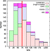 |
Fig. 1 Histogram distribution of the signal-to-noise ratios for all spectra from all four spectrographs. The red solid line marks the signal-to-noise ratio limit of 75. |
3 Method
We adapted the method described in Passegger et al. (2016), who determined the fundamental stellar parameters effective temperature Teff, surface gravity logg, and metallicity [Fe/H] for four M dwarfs using the latest grid of PHOENIX model spectra presented by Husser et al. (2013). The PHOENIX code was developed by Hauschildt (1992, 1993) and has been considerably improved since then (e.g. Hauschildt et al. 1997; Hauschildt & Baron 1999; Claret et al. 2012; Husser et al. 2013). The code can generate 1D model atmospheres of plane-parallel or spherically symmetric stars and degenerate objects (late-type stars as well as brown dwarfs, white dwarfs, and giants), accretion discs, and expanding envelopes of novae and supernovae. Synthetic spectra can be calculated in 1D and 3D using local thermal equilibrium (LTE) or non-LTE radiative transfer for any desired spectral resolution.
This new PHOENIX-ACES model grid was especially designed for modelling spectra of cool dwarfs, because it uses a new equation of state to improve the calculations of molecule formation in cool stellar atmospheres. This allows good fitting of the γ- and ϵ-TiO bands (λhead 705 nm and λhead 843 nm, respectively), which are very sensitive to effective temperature. The ϵ-TiO band is especially sensitive to temperatures lower than 3000 K. The models use solar abundances from Asplund et al. (2009). Models with [α/Fe] ≠ 0 are only available for Teff > 3500 K and 3 ≤ [Fe∕H] ≤ 0. Therefore, we focus our analysis on models with [α∕Fe] = 0. In this context, Veyette et al. (2016) reported a significant effect on the spectra of M dwarfs if abundances of other elements are varied. They found that a change in the C/O ratio influences the pseudo-continuum by changing TiO and H2 O opacities. In our study, however, we focused on the application of the latest PHOENIX-ACES models, with [Fe/H] being the only free abundance parameter.
We slightly modified the algorithm developed by Passegger et al. (2016). Because all stars in our sample have effective temperatures hotter than 3000 K, we only included the γ-TiO band in our fitting. Passegger et al. (2016) also showed that the K I and Na I doublets around 768 and 819 nm, respectively, are suitable for surface gravity and metallicity determination. Since the K I line at 766.5 nm is contaminated by telluric lines, we decided to exclude it from the fitting. We excluded the Ca II doublet at 850.0 and 866.4 nm as well, because these lines are not well reproduced by the models: they are formed in the chromosphere and can show emission when the star is magnetically active.The Na I doublet around 819 nm was previously used because of its high pressure sensitivity (see Passegger et al. 2016). In a detailed analysis of the first results of our large sample, we found a degeneracy in the strength and width of the Na I doublet over a wide parameter range, which made it difficult to distinguish between a cool-metal poor and a hot-metal rich model. Therefore we excluded this doublet from our analysis. The γ-TiO band and Mg I line (λ 880.9 nm) were found to be more suitable for metallicity determination, and they were therefore assigned higher weights during fitting. As an example, Fig. 2 presents χ2 maps of the Mg I line for one of our stars in the Teff – logg and Teff–[Fe/H] plane, where a strong dependency on metallicity can be seen. A χ2 minimisation is used to determine the best fit of the models to the observed spectra. As described in Passegger et al. (2016), the procedure is divided into two steps, which are described in the following.
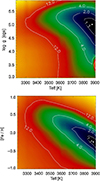 |
Fig. 2 χ2 map of the Mg I line for BR Psc (GJ 908) with χ2 contour values. The upper panel shows the Teff– logg plane, and the lower panel the Teff–[Fe/H] plane. The minimum for this line is indicated with a white dot. |
3.1 Coarse grid search
In a first step, we used the coarsely spaced grid of the model spectra in a wide range around the expected parameters of the star. To match the instrumental resolutions, the model spectra were first convolved with a Gaussian. Then the average flux of the models and the observed spectrum was normalised to unity by assuming a pseudo-continuum for each wavelength range. Next, the models were interpolated to match the wavelength grid of the observed spectrum, so that each wavelength point of each model spectrum could be compared to the stellar spectrum. The value of χ2 was calculated to find a rough global minimum. This was done for different wavelength ranges between 705.0 and 820.5 nm. The parameters for the three best minima were given as an output in order to provide different starting values for the downhill simplex in the next step.
3.2 Fine grid search
In the second step, the region around each global minimum was explored on a finer grid. The wavelength range was extended to 883.5 nm to include some titanium and iron lines. An overview of all regions and lines used for fitting is presented in Table 2. To reduce the number of free parameters in the fit, we used the values of projected rotation velocity v sin i determined by Jeffers et al. (2018) using cross-correlation. To account for v sin i, the model spectra were broadened using a broadening function. The function determined the effect on the line spread function caused by stellar rotation. The resulting line spread function was convolved with the model spectrum. In contrast to Passegger et al. (2016), who used the IDL curvefit function, we used a downhill simplex method for fitting, which we found to be more robust on large samples. The downhill simplex used linear interpolation between the model grid points to explore the parameter space in detail. A χ2 minimisation finds the best-fit model. This was done for all three minima found in the previous step. The parameters with the best χ2 were selected as results.
From the first results for our sample, the fits showed very good agreement between models and observed spectra. However, we found that the values of logg and [Fe/H] were much higher than expected for main-sequence M dwarfs; the log g was between 5.5 and 6.0, and most metallicities were super-solar, with values of up to 1.0 dex. Moreover, we found exceptionally low log g of 3.0 with metallicities of − 1.0 dex for some stars. In both cases the fitted models agreed very well with the data. The results of obviously wrong parameter values can be explained by a degeneracy between Teff, log g, and [Fe/H], which is displayed in Fig. 3. Especially, the Teff –[Fe/H] map shows a largely extended minimum. To break this degeneracy, we decided to determine log g using an independent method.
Baraffe et al. (1998) presented evolutionary models for low-mass stars up to 1.4 M⊙. A new version of these models was published by Baraffe et al. (2015) using updated solar abundances. However, the Baraffe et al. (1998) and Baraffe et al. (2015) Teff– logg relations are consistent with each other in the temperature range of M dwarfs, therefore we used the Baraffe et al. (1998) version. Amongst other parameters, they provided effective temperatures and surface gravities for different stellar ages and metallicities of 0.0 and −0.5 dex. Unfortunately, the ages of the stars in the CARMENES target sample are not yet well constrained. This will be the topic of upcoming papers. A preliminary kinematics and activity analysis of the sample to qualitatively estimate ages was carried out by Cortés-Contreras (2016). Therefore, we assumed an age of 5 Gyr for the whole sample. This seems to be a good guess even for younger stars because once M dwarfs reach the main sequence they evolve extremely slowly (e.g. Burrows et al. 1997; Laughlin et al. 1997). This is also reflected in the Baraffe et al. (1998) relations, which agree within 0.02 dex in logg for ages between 1 and 7 Gyr in the temperature range of M dwarfs up to 4000 K. In the algorithm the downhill simplex can vary Teff and metallicity. Based on this, logg was determined from the Teff– logg relations. Metallicities between 0.0 and −0.5 dex were linearly interpolated from the relations to estimate logg. For metallicities higher than 0.0 dex or lower than −0.5 dex, the values were extrapolated. Because the differences in logg depending on metallicity are small (no larger than 0.20 dex between metallicities 0.0 and −0.5 dex), we expect the uncertainty from the interpolation and extrapolation to be negligible compared to the uncertainty coming from the fitting. From these three parameters, the corresponding PHOENIX model was interpolated and the χ2 was calculated. Figure 4 shows a co-added CARMENES spectrum of a typical M1 V star with the best-fit model, including the lines and regions we used for fitting.
Wavelength regions and lines used for the χ2 fitting.
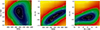 |
Fig. 3 χ2 maps for BR Psc (GJ 908) for different combinations of stellar parameters. The global minimum is indicated with a white dot. |
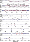 |
Fig. 4 Co-added CARMENES spectrum of the M1 V star GX And (black) and the best-fit model (blue: whole fit, and red: regions used for χ2 minimisation). |
4 Results and discussion
Table A.1 presents the fundamental parameters of our target sample. It includes the CARMENES identifiers, spectral types from Carmencita, Teff, logg, and [Fe/H] derived in this study, vsini determined by Jeffers et al. (2018), masses from Carmencita (see Sect. 4.4), a flag for Ca II emission, and the instrument with which the analysed spectrum was observed. We applied the method for error estimation as given in Passegger et al. (2016). They estimated errors by adding Poisson noise to 1400 model spectra with random parameter distributions to simulate S/N ~ 100 and applied their algorithm to recover the input parameters. Using this method, we derived uncertainties of 51 K for Teff, 0.07 dex for logg, and 0.16 dex for [Fe/H], which are consistent with typical uncertainties in literature. We confirmed this statement by calculating deviations between our results and literature values (σexp) together with the corresponding standard deviation (σΔ). The numbers are presented in Table 3, showing that σΔ are smaller than the expected deviations σexp for the different literature samples.
Expected errors and deviations in Teff, log g, and [Fe/H] of our results and the literature.
4.1 Effective temperature
The histogram distributions for all parameters for all 300 stars are presented in Fig. 5. The temperature distribution (left panel) shows that most of the stars in our sample have temperatures of between 3200 and 3800 K, corresponding to spectral types ranging from M0.0 to M5.0 V. Figure 6 gives a comparison of 98 stars that overlap with the samples of RA12, Maldonado et al. (2015, hereafter Ma15), and GM14. Ma15 determined effective temperature and metallicity from optical spectra using pseudo-equivalent widths. In general, most of our results agree with the literature values within the error bars. However, there is one group of outliers at the cool end of the sample. This group is represented by results from RA12, who determined temperatures using the H2 O-K2 index calibrated with BT-Settl models of solar metallicity. They derived temperatures that are cooler than ours by about 200 K. Two more outliers are located around 3550 K (GJ 752A) and 3650 K (BR Psc/GJ 908), for which RA12 determined considerably hotter temperatures of 3789 and 3995 K, respectively. However, our temperatures are consistent with those derived by Ma15 and GM14, which makes the result of RA12 discrepant. A small “bump” can be found between 3550 and 3700 K, where GM14 tended to derive slightly higher temperatures than we do. For other stars in Fig. 6, the values are mostly consistent with our results.
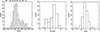 |
Fig. 5 Histogram distributions of Teff (left panel) together with spectral types from Kenyon & Hartmann (1995) on the upper x-axis, log g (middle panel), and [Fe/H] (right panel) for our 300 stars. |
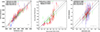 |
Fig. 6 Comparison between values from our sample and literature values for Teff (left panel), logg (middle panel), and [Fe/H] (right panel). The black line indicates the 1:1 relation. The grey lines indicate the 1σ deviation of 51 K, 0.07 dex in logg, and 0.16 dex in [Fe/H]. The black dots with error bars in the lower right corner of each plot show the uncertainties of this work. |
4.2 Surface gravity
The middlepanel of Fig. 5 presents the log g distribution for our sample. Ma15 determined logg for early-M dwarfs using stellar masses from photometric relations and radii from an empirical mass–radius relation that combines interferometry (von Braun et al. 2014; Boyajian et al. 2012) and data from low-mass eclipsing binaries (Hartman et al. 2015). A comparison of those stars that we have in common is presented in the middle panel of Fig. 6. The grey lines indicate a 1σ deviation of 0.07 dex. We calculated logg for the sample of GM14 from the provided masses and radii. The uncertainties were derived with error propagation from the uncertainties in mass and radius. We included logg values based on interferometric radius measurements from Boyajian et al. (2012). We derived the log g in the same way as for GM14. Our results are consistent with the logg values from Ma15, which mostly lie between 4.6 and 5.0 dex. Most of the interferometrically based log g also agree with our values. This is expected since they are constrained by the Teff – logg relations. It also shows consistency between the empirical radius calibration of Ma15 and theoretical models. However, when we compare our logg values with those of GM14, we find some offset. At the lower end of the plot, we derive higher values than GM14. Because log g depends on Teff in our calculation, this trend is consistent with the bump found in the temperature plot. The values of Boyajian et al. (2012) slightly follow the same trend as GM14, although the sample is too small to draw a definite conclusion.
4.3 Metallicity
The right panel of Fig. 5 displays the metallicity distribution of our results, centred on solar metallicity. The right panel of Fig. 6 shows a comparison of the stars that we have in common with RA12, Ma15, and GM14. Their metallicity measurements range from −0.6 to 0.4 dex, whereas our results only range from −0.4 to almost 0.2 dex. This indicates that the metallicity is more difficult to constrain than the other parameters, and that different methods could give noticeably different results. On the other hand, we find that even for spectra for which the parameters agree with the literature, some lines, such as Ti I (λ 846.9 and 867.77 nm) and Fe I (λ 867.71 and 882.6 nm), are too deep. A possible explanation might be the contrast between the line and the continuum so that the models still cannot reproduce the correct line depths. On the other hand, we used models with element abundances fixed to solar. A change in [α/Fe] or [Ti/Fe] might improve the fit for some stars. A more extensive study on the performance of the models themselves, probably including different element abundances, is necessary to completely understand their behaviour.
4.4 Relation of spectral type, mass, and temperature
We present the relation between stellar mass and effective temperature in Fig. 7, and the metallicities are colour-coded. The thick black line represents the theoretical relation from Baraffe et al. (1998) for an age of 5 Gyr and solar metallicity. The masses were calculated by combining mass–luminosity relations from Delfosse et al. (2000, for 4.5 mag < Ks < 5.29 mag) and Benedict et al. (2016, for 5.29 mag < Ks < 10 mag), with the magnitudes taken from the Carmencita database (see Alonso-Floriano et al. 2015). In this plot, stars with super-solar metallicity should lie below the relation reported by Baraffe et al. (1998) and stars with sub-solar metallicity should lie above this relation. As can be seen, most of the stars lie below the theoretical prediction. This can be due to several reasons: our Teff s are systematically underestimated, our metallicities are slightly lower than expected, or the determined stellar masses are overestimated. Based on the literature comparison in Sect. 4.1, we can exclude the former two. Since Delfosse et al. (2000) did not provide errors for their mass–luminosity relation, we assumed an average uncertainty of 10% in mass over the whole mass range, which is of the same order as the errors from Benedict et al. (2016). Within this range, our values agree with the theoretical relation of Baraffe et al. (1998). Some obvious outliers are identified by numbers and are discussed in more detail later.
Figure 8 shows the effective temperatures of all stars as a function of their spectral type; the spectral types are taken from the Carmencita database. The green stars show the expected temperature-spectral type relation as presented by Kenyon & Hartmann (1995). The authors computed effective temperatures, colours, spectral types, and bolometric corrections for main-sequence stars from B0 to M6 after an extensive literature search. Their temperatures fit our results for solar metallicities well. The large spread in temperature for each spectral type is caused by different metallicities, which are colour-coded. This indicates that stars of the same spectral type have higher temperatures if they are more metal-rich, or in other words: for the same effective temperature, the spectral type decreases with increasing metallicity. This can be explained with an increase in opacity in the optical with increasing metallicity, mainly dominated by TiO and VO molecular bands. The peak of the energy distribution is therefore shifted towards longer wavelengths and makes the star appear redder, that is, of later spectral type. This effect has been discussed in more detail by Delfosse et al. (2000); Chabrier & Baraffe (2000). A similar trend was found by Mann et al. (2015), who derived empirical relations between Teff, [Fe/H], radii, and luminosities. They showed that the radius increases with metallicity for a fixed temperature (see their Fig. 23).
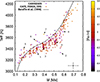 |
Fig. 7 Effective temperature as a function of stellar mass. The determined metallicities of the stars are colour-coded. The different symbols present stars observed with CARMENES or CAFE, FEROS, and HRS. The thick black line shows the theoretical relation for solar metallicity from Baraffe et al. (1998). An average uncertainty of 10% in mass is indicated by the black dot with error bars in the lower right corner. The eight outliers discussed in Sect. 4.5 are labelled. |
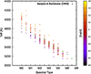 |
Fig. 8 Effective temperature as a function of spectral type. The determined metallicities of the stars are colour-coded. The green stars indicate the expected temperatures for each spectral type computed by Kenyon & Hartmann (1995). |
4.5 Analysis of outliers
In the following, eight outliers found in the mass–temperature plot of Fig. 7 are discussed in more detail. We selected them because their Teff or metallicity clearly deviate from the relation reported by Baraffe et al. (1998).
(1) J03430+459
This star was observed with HRS. The best-fit model agrees moderately well with the observed spectrum, with small deviations in the TiO bandheads and some Ti I and Fe I lines. Alonso-Floriano et al. (2015) measured a pseudo-equivalent width of −0.7 Å for Hα. Newton et al. (2017) also reported that this star is slightly active. This could explain the deviations in the Fe I and Ti I lines, which are sensitive to magnetic Zeeman splitting. A change in [Ti/Fe] or [α/Fe], on the other hand, could also be responsible for a deviation in the fit of Ti I lines.
(2) J04544+650
For this star we also used HRS spectra to determine the parameters. The star is magnetically active, has an Hα pseudo-equivalent width of −13.9 Å (Alonso-Floriano et al. 2015), and shows Ca II emission. We find deviations in some Ti I and Fe I lines, which could explain the deviation in metallicity.
(3) J05078+179
This star was observed with FEROS. The best spectrum has an S∕N of 104. The star shows Hα emission with a pseudo-equivalent width of −0.7 Å (Jeffers et al. 2018). The activity also causes distortion in other lines (e.g. some Fe I and Ti I lines). Here, the deviations in some Ti I lines might also be caused by Ti abundances that are different from solar, and this might in turn explain the low metallicity.
(4) J11201−104
We analysed CARMENES spectra of this star and found it to be too metal-poor in the mass–Teff plot. The star has strong Ca II emission. Alonso-Floriano et al. (2015) reported an Hα pseudo-equivalent width of −3.3 Å. The magnetic activity might explain the deviations in the Fe I lines here as well, and therefore also the deviation in the determined lower metallicity.
(5) J18346+401
For this star we used a co-added CARMENES spectrum to derive the parameters. The best model fits the observed spectrum very well. The resulting temperature of 3391 K is comparable to the temperature measured by Gaidos & Mann (2014) from near-infrared data. However, Gaidos & Mann (2014) determined a metallicity of 0.42 dex, whereas we obtained a more metal-poor value of 0.09 dex. The line depth is well fitted in our spectrum. We also derived a lower χ2 compared to the parameter set of Gaidos & Mann (2014). The star is not known to be active and does not show any Ca II emission either. Considering all this information, we cannot explain the measured low metallicity satisfactorily.
(6) J21057+502
We analysed HRS spectra for this star and found good agreement between the observed spectra and the best-fit models. Our derived temperature of 3543 K is about 100 K too hot for the spectral type M3.5. However, the χ2 -map shows a large extended minimum in the Teff – logg–[Fe/H] planes, which reaches from almost 3700 K and +0.5 [Fe/H] down to 3500 K and +0.1 [Fe/H], making the derived parameters less significant. Cortés-Contreras (2016) reported from an analysis of the stellar kinematics that this star is part of the young disc and a probable member of the local association, which is 10–150 Myr old. The models of Baraffe et al. (1998) show that using an age of 5 Gyr for a star younger than 0.5 Gyr can lead to an increase in Teff of 50–100 K. Accounting for these two circumstances results in a slightly lower temperature and metallicity, which causes the star to fit the mass–Teff relation better.
(7) J21152+257
The fit to this co-added CARMENES spectrum is good: we find only minor deviations between observed and fitted lines, especially for the TiO-band. The star is inactive and does not show any signs of emission in Hα or Ca II. The determined temperature of 3657 K is about 200 K hotter than expected for the stated spectral type M3. The χ2 -map has a large extended and deep minimum here as well, which is located between about 3800 K and +0.5 [Fe/H], and 3550 K and +0.1 [Fe/H]. This might explain the too high temperature and metallicity.
(8) J21221+229
The parameters of this star were also derived from a co-added CARMENES spectrum, for which the model fit is very good. The star is not active, and the spectral type M1 corresponds to the fitted temperature of 3704 K. We are unable to explain the deviation in Fig. 7 for this star.
5 Summary
CARMENES is a new instrument at the Calar Alto observatory that simultaneously takes high-resolution spectra in the visible and near-infrared wavelength ranges. Its aim is to search for Earth-sized planets in the habitable zone around M dwarfs.
We provided precise parameters from PHOENIX-ACES model fits for effective temperature, surface gravity, and metallicity for 300 M dwarfs, which is the largest sample of M dwarfs investigated with high-resolution spectroscopy so far. It is important not only for CARMENES, but also for future exoplanet surveys, since knowing stellar fundamental parameters is essential for characterising an orbiting planet. Moreover, accurate metallicities are crucial for theories of planet formation around low-mass stars and give information on the chemical evolution of the Galaxy.
Our work presents a test of the new PHOENIX-ACES models on a large sample of low-mass stars and points out inconsistencies in line depths and metallicity determination. This analysis also serves as a comparison of methods using low- and high-resolution spectra for stellar parameter determination. Table 4 summarises the different literature approaches for determining stellar parameters. It illustrates that in contrast to other comparable studies, we used high-resolution spectra and fitting of the latest model atmospheres. Comparisons with literature values for some of the target stars showed that we achieve very good agreement in the temperatures. For the metallicity we find an overall distribution that shows mainly sub-solar values and peaks between 0.0 and −0.1 dex, which agrees with findings from Gaidos & Mann (2014, see their Fig. 1). Our values are consistent with the literature within 1σ, although there is no obvious correlation between our values and literature results. This might indicate an inconsistency in metallicity determination as such and may require further improvement of methods and models. Simultaneous fitting of allthree parameters did not provide reliable results for all sample stars. Therefore, we determined log g from temperature- and metallicity-dependent relations from evolutionary models assuming an average age of 5 Gyr for our sample. However, we showed that our results in logg agree well with interferometric observations by Boyajian et al. (2012), which also serves as an evaluation of theoretical evolutionarymodels and observations.
To confirm our results, we performed χ2 fits with our spectra and models with parameters determined by GM14, Ma15, and RA12. We compared the χ2 s with those resulting from fits with our derived parameters and found the smallest χ2 for 92% of the fits with our parameters. For the remaining 8%, the literature parameters agree with ours within their errors. This confirms that our method, using the latest PHOENIX-ACES models, provides the best-fit parameters to our observations. It shows that our method has the potential to derive accurate stellar parameters for M dwarfs. This contributes to the most extensive catalogue of M-dwarf parameters so far. However, we also showed that there are still some shortcomings in synthetic models for low-temperature atmospheres, although they have significantly improved in the past decade. While the PHOENIX-ACES models fit observed spectra very well and show only negligible deviations within the noise level, we can find some discrepancies. From the fit, the full line depth is not represented for some lines, which might be the reason for the differences in metallicity we found compared to literature values. A small offset in metallicity is also depicted in Fig. 7. Our results for solar metallicity lie systematically below the mass–luminosity relation of Baraffe et al. (1998), but largely follow the theoretical prediction. Further detailed analysis of the models is necessary for better understanding the metallicity dependency.
We identified eight outliers; four of them show activity either in Hα or Ca II. Magnetic activity can distort line profiles by Zeeman splitting (e.g. Hébrard et al. 2014; Reiners et al. 2013), which could explain deviations in some sensitive Fe I and Ti I lines. Furthermore, a Ti and α-element abundance different from the Sun might also cause deviations in the Ti I lines. Two outliers are caused by large extended and deep minima in the Teff – logg–[Fe/H] planes. One of these stars is believed to have an age younger than 0.5 Gyr (Cortés-Contreras 2016), which results in a too high temperature when using the models of Baraffe et al. (1998) for 5 Gyr. For two outliers we were not able to provide any explanation.
Finally, an accurate age determination of the sample stars would be helpful. This topic will be addressed in subsequent CARMENES papers. The S∕N also has a significant influence on the parameter determination, which makes a high S∕N preferable when using the method we presented here. A great advantage of the new CARMENES instrument is its capability to provide simultaneous observations in the visible and near-infrared wavelength range. A detailed investigation of spectra in both ranges is desirable to better understand M-dwarf atmospheres. The analysis of CARMENES near-infrared spectra will be presented in forthcoming works.
Summary of literature approaches for the stellar parameter determination.
Acknowledgements
We thank the anonymous referee for her/his comments that helped to improve the quality of this paper. VMP wouldlike to thank Denis Shulyak for fruitful discussions. CARMENES is an instrument for the Centro Astronómico Hispano-Alemán de Calar Alto (CAHA, Almería, Spain). CARMENES is funded by the German Max-Planck-Gesellschaft (MPG), the Spanish Consejo Superior de Investigaciones Científicas (CSIC), the European Union through FEDER/ERF FICTS-2011-02 funds, and the members of the CARMENES Consortium (Max-Planck-Institut für Astronomie, Instituto de Astrofísica de Andalucía, Landessternwarte Königstuhl, Institut de Ciències de l’Espai, Institut für Astrophysik Göttingen, Universidad Complutense de Madrid, Thüringer Landessternwarte Tautenburg,Instituto de Astrofísica de Canarias, Hamburger Sternwarte, Centro de Astrobiología and Centro Astronómico Hispano-Alemán), with additional contributions by the Spanish Ministry of Economy, the German Science Foundation through the Major Research Instrumentation Programme and DFG Research Unit FOR2544 “Blue Planets around Red Stars”, the Klaus Tschira Stiftung, the states of Baden-Württemberg and Niedersachsen, and by the Junta de Andalucía. IR acknowledges support from the Spanish Ministry of Economy and Competitiveness (MINECO) through grant ESP2014-57495-C2-2-R. VJSB is supported by programme AYA2015-69350-C3-2-P from Spanish Ministry of Economy and Competitiveness (MINECO) Based on observations collected at the Centro Astronómico Hispano Alemán (CAHA) at Calar Alto, operated jointly by the Max–Planck Institut für Astronomie and the Instituto de Astrofísica de Andalucía. This research has made use of the VizieR catalogue access tool, CDS, Strasbourg, France. The original description of the VizieR service was published in A&AS 143, 23.
Appendix A: Table of parameters
Basic astrophysical parameters of investigated stars.
References
- Aceituno, J., Sánchez, S. F., Grupp, F., et al. 2013, A&A, 552, A31 [NASA ADS] [CrossRef] [EDP Sciences] [Google Scholar]
- Allard, F., Homeier, D., & Freytag, B. 2012a, Phil. Trans. R. Soc. London, Ser. A, 370, 2765 [Google Scholar]
- Allard, F., Homeier, D., Freytag, B., & Sharp, C. M. 2012b, in eds. C. Reylé, C. Charbonnel, & M. Schultheis, EAS Pub. Ser., 57, 3 [Google Scholar]
- Alonso-Floriano, F. J., Morales, J. C., Caballero, J. A., et al. 2015, A&A, 577, A128 [NASA ADS] [CrossRef] [EDP Sciences] [Google Scholar]
- Asplund, M., Grevesse, N., Sauval, A. J., & Scott, P. 2009, ARA&A, 47, 481 [NASA ADS] [CrossRef] [Google Scholar]
- Baraffe, I., Chabrier, G., Allard, F., & Hauschildt, P. H. 1998, A&A, 337, 403 [NASA ADS] [Google Scholar]
- Baraffe, I., Homeier, D., Allard, F., & Chabrier, G. 2015, A&A, 577, A42 [NASA ADS] [CrossRef] [EDP Sciences] [Google Scholar]
- Benedict, G. F., Henry, T. J., Franz, O. G., et al. 2016, AJ, 152, 141 [NASA ADS] [CrossRef] [Google Scholar]
- Boyajian, T. S., von Braun, K., van Belle, G., et al. 2012, ApJ, 757, 112 [NASA ADS] [CrossRef] [Google Scholar]
- Browning, M. K., Basri, G., Marcy, G. W., West, A. A., & Zhang, J. 2010, AJ, 139, 504 [NASA ADS] [CrossRef] [Google Scholar]
- Burrows, A., Marley, M., Hubbard, W. B., et al. 1997, ApJ, 491, 856 [NASA ADS] [CrossRef] [Google Scholar]
- Caballero, J. A., Cortés-Contreras, M., Alonso-Floriano, F. J., et al. 2016a, 19th Cambridge Workshop on Cool Stars, Stellar Systems, and the Sun (CS19), 148 [Google Scholar]
- Caballero, J. A., Guàrdia, J., López del Fresno, M., et al. 2016b, in Observatory Operations: Strategies, Processes, and Systems VI, Proc. SPIE, 9910, 99100E [Google Scholar]
- Chabrier, G. & Baraffe, I. 2000, ARA&A, 38, 337 [NASA ADS] [CrossRef] [Google Scholar]
- Claret, A., Hauschildt, P. H., & Witte, S. 2012, A&A, 546, A14 [NASA ADS] [CrossRef] [EDP Sciences] [Google Scholar]
- Cortés-Contreras, M. 2016, Ph.D. thesis, Universidad Complutense de Madrid, Spain [Google Scholar]
- Cortés-Contreras, M., Béjar, V. J. S., Caballero, J. A., et al. 2017, A&A, 597, A47 [NASA ADS] [CrossRef] [EDP Sciences] [Google Scholar]
- Delfosse, X., Forveille, T., Ségransan, D., et al. 2000, A&A, 364, 217 [NASA ADS] [Google Scholar]
- Gaidos, E. & Mann, A. W. 2014, ApJ, 791, 54 [NASA ADS] [CrossRef] [Google Scholar]
- Gustafsson, B., Edvardsson, B., Eriksson, K., et al. 2008, A&A, 486, 951 [NASA ADS] [CrossRef] [EDP Sciences] [Google Scholar]
- Hartman, J. D., Bayliss, D., Brahm, R., et al. 2015, AJ, 149, 166 [NASA ADS] [CrossRef] [Google Scholar]
- Hauschildt, P. H. 1992, J. Quant. Spec. Rad. Transf., 47, 433 [NASA ADS] [CrossRef] [Google Scholar]
- Hauschildt, P. H. 1993, J. Quant. Spec. Rad. Transf., 50, 301 [NASA ADS] [CrossRef] [Google Scholar]
- Hauschildt, P. H. & Baron, E. 1999, J. Comput. Appl. Math., 109, 41 [NASA ADS] [CrossRef] [Google Scholar]
- Hauschildt, P. H., Baron, E., & Allard, F. 1997, ApJ, 483, 390 [NASA ADS] [CrossRef] [Google Scholar]
- Hébrard, É. M., Donati, J.-F., Delfosse, X., et al. 2014, MNRAS, 443, 2599 [NASA ADS] [CrossRef] [Google Scholar]
- Houdebine, E. R. 2010, MNRAS, 407, 1657 [NASA ADS] [CrossRef] [Google Scholar]
- Husser, T.-O., Wende-von Berg, S., Dreizler, S., et al. 2013, A&A, 553, A6 [NASA ADS] [CrossRef] [EDP Sciences] [Google Scholar]
- Jeffers, S. V., Schöfer, P., Lamert, A., et al. 2018, A&A, 614, A76 [Google Scholar]
- Kaufer, A., Wolf, B., Andersen, J., & Pasquini, L. 1997, The Messenger, 89, 1 [NASA ADS] [Google Scholar]
- Kenyon, S. J. & Hartmann, L. 1995, ApJS, 101, 117 [NASA ADS] [CrossRef] [Google Scholar]
- Laughlin, G., Bodenheimer, P., & Adams, F. C. 1997, ApJ, 482, 420 [NASA ADS] [CrossRef] [Google Scholar]
- Lindgren, S. & Heiter, U. 2017, A&A, 604, A97 [NASA ADS] [CrossRef] [EDP Sciences] [Google Scholar]
- Maldonado, J., Affer, L., Micela, G., et al. 2015, A&A, 577, A132 [NASA ADS] [CrossRef] [EDP Sciences] [Google Scholar]
- Mann, A. W., Brewer, J. M., Gaidos, E., Lépine, S., & Hilton, E. J. 2013, AJ, 145, 52 [NASA ADS] [CrossRef] [Google Scholar]
- Mann, A. W., Feiden, G. A., Gaidos, E., Boyajian, T., & von Braun K. 2015, ApJ, 804, 64 [NASA ADS] [CrossRef] [Google Scholar]
- Newton, E. R., Irwin, J., Charbonneau, D., et al. 2017, ApJ, 834, 85 [NASA ADS] [CrossRef] [Google Scholar]
- Passegger, V. M. 2017, Ph.D. thesis, Georg-August-Universität Göttingen, Germany [Google Scholar]
- Passegger, V. M., Wende-von Berg, S., & Reiners, A. 2016, A&A, 587, A19 [NASA ADS] [CrossRef] [EDP Sciences] [Google Scholar]
- Quirrenbach, A., Amado, P. J., Caballero, J. A., et al. 2016, in Ground-based and Airborne Instrumentation for Astronomy VI, Proc. SPIE, 9908, 990812 [Google Scholar]
- Quirrenbach, A., Amado, P. J., Caballero, J. A., et al. 2014, in Ground-based and Airborne Instrumentation for Astronomy V, SPIE Conf. Ser. 9147, 91471F [Google Scholar]
- Rajpurohit, A. S., Reylé, C., Allard, F., et al. 2013, A&A, 556, A15 [NASA ADS] [CrossRef] [EDP Sciences] [Google Scholar]
- Reiners, A., Joshi, N., & Goldman, B. 2012, AJ, 143, 93 [NASA ADS] [CrossRef] [Google Scholar]
- Reiners, A., Shulyak, D., Anglada-Escudé, G., et al. 2013, A&A, 552, A103 [NASA ADS] [CrossRef] [EDP Sciences] [Google Scholar]
- Reiners, A., Zechmeister, M., Caballero, J. A., et al. 2018, A&A, 612, A49 [Google Scholar]
- Rojas-Ayala, B., Covey, K. R., Muirhead, P. S., & Lloyd, J. P. 2012, ApJ, 748, 93 [NASA ADS] [CrossRef] [Google Scholar]
- Souto, D., Cunha, K., García-Hernández, D. A., et al. 2017, ApJ, 835, 239 [NASA ADS] [CrossRef] [Google Scholar]
- Stahl, O., Kaufer, A., & Tubbesing, S. 1999, in Optical and Infrared Spectroscopy of Circumstellar Matter, eds. E. Guenther, B. Stecklum, & S. Klose, ASP Conf. Ser., 188, 331 [NASA ADS] [Google Scholar]
- Tull, R. G., MacQueen, P. J., Good, J., Epps, H. W., & HET HRS, Team. 1998, in American Astronomical Society Meeting Abstracts, Bull. Am. Astron. Soc., 30, 1263 [NASA ADS] [Google Scholar]
- Valenti, J. A. & Piskunov, N. 1996, A&AS, 118, 595 [NASA ADS] [CrossRef] [EDP Sciences] [Google Scholar]
- Veyette, M. J., Muirhead, P. S., Mann, A. W., & Allard, F. 2016, ApJ, 828, 95 [NASA ADS] [CrossRef] [Google Scholar]
- Veyette, M. J., Muirhead, P. S., Mann, A. W., et al. 2017, ApJ, 851, 26 [NASA ADS] [CrossRef] [Google Scholar]
- von Braun, K., Boyajian, T. S., van Belle, G. T., et al. 2014, MNRAS, 438, 2413 [NASA ADS] [CrossRef] [Google Scholar]
- Zechmeister, M., Reiners, A., Amado, P. J., et al. 2017, A&A, 609, A12 [Google Scholar]
All Tables
Expected errors and deviations in Teff, log g, and [Fe/H] of our results and the literature.
All Figures
|
Fig. 1 Histogram distribution of the signal-to-noise ratios for all spectra from all four spectrographs. The red solid line marks the signal-to-noise ratio limit of 75. |
| In the text | |
|
Fig. 2 χ2 map of the Mg I line for BR Psc (GJ 908) with χ2 contour values. The upper panel shows the Teff– logg plane, and the lower panel the Teff–[Fe/H] plane. The minimum for this line is indicated with a white dot. |
| In the text | |
|
Fig. 3 χ2 maps for BR Psc (GJ 908) for different combinations of stellar parameters. The global minimum is indicated with a white dot. |
| In the text | |
|
Fig. 4 Co-added CARMENES spectrum of the M1 V star GX And (black) and the best-fit model (blue: whole fit, and red: regions used for χ2 minimisation). |
| In the text | |
|
Fig. 5 Histogram distributions of Teff (left panel) together with spectral types from Kenyon & Hartmann (1995) on the upper x-axis, log g (middle panel), and [Fe/H] (right panel) for our 300 stars. |
| In the text | |
|
Fig. 6 Comparison between values from our sample and literature values for Teff (left panel), logg (middle panel), and [Fe/H] (right panel). The black line indicates the 1:1 relation. The grey lines indicate the 1σ deviation of 51 K, 0.07 dex in logg, and 0.16 dex in [Fe/H]. The black dots with error bars in the lower right corner of each plot show the uncertainties of this work. |
| In the text | |
|
Fig. 7 Effective temperature as a function of stellar mass. The determined metallicities of the stars are colour-coded. The different symbols present stars observed with CARMENES or CAFE, FEROS, and HRS. The thick black line shows the theoretical relation for solar metallicity from Baraffe et al. (1998). An average uncertainty of 10% in mass is indicated by the black dot with error bars in the lower right corner. The eight outliers discussed in Sect. 4.5 are labelled. |
| In the text | |
|
Fig. 8 Effective temperature as a function of spectral type. The determined metallicities of the stars are colour-coded. The green stars indicate the expected temperatures for each spectral type computed by Kenyon & Hartmann (1995). |
| In the text | |
Current usage metrics show cumulative count of Article Views (full-text article views including HTML views, PDF and ePub downloads, according to the available data) and Abstracts Views on Vision4Press platform.
Data correspond to usage on the plateform after 2015. The current usage metrics is available 48-96 hours after online publication and is updated daily on week days.
Initial download of the metrics may take a while.