| Issue |
A&A
Volume 615, July 2018
|
|
|---|---|---|
| Article Number | A4 | |
| Number of page(s) | 25 | |
| Section | Stellar atmospheres | |
| DOI | https://doi.org/10.1051/0004-6361/201731839 | |
| Published online | 03 July 2018 | |
Carbon line formation and spectroscopy in O-type stars
Universitätssternwarte München,
Scheinerstr. 1,
81679
München,
Germany
e-mail: luiz@usm.uni-muenchen.de
Received:
27
August
2017
Accepted:
5
December
2017
Context. The determination of chemical abundances constitutes a fundamental requirement for obtaining a complete picture of a star. Particularly in massive stars, CNO abundances are of prime interest, due to the nuclear CNO-cycle, and various mixing processes which bring these elements to the surface. The precise determination of carbon abundances, together with N and O, is thus a key ingredient for understanding the different phases of stellar evolution.
Aims. We aim to enable a reliable carbon spectroscopy for our unified non-LTE atmosphere code FASTWIND.
Methods. We have developed a new carbon model atom including C II/III/IV/V, and we discuss specific problems related to carbon spectroscopy in O-type stars. We describe different tests we have performed to examine the reliability of our implementation, and investigate which mechanisms influence the carbon ionization balance. By comparing with high-resolution spectra from six O-type stars, we verified to what extent observational constraints can be reproduced by our new carbon line synthesis.
Results. Carbon lines are even more sensitive to a variation of Teff, log g, and Ṁ, than hydrogen and helium lines. We are able to reproduce most of the observed lines from our stellar sample, and to estimate those specific carbon abundances which bring the lines from different ions into agreement (three stages in parallel for cool objects, two for intermediate O-types). For hot dwarfs and supergiants earlier than O7, X-rays from wind-embedded shocks can have an impact on the synthesized line strengths, particularly for C IV, potentially affecting the abundance determination. Dielectronic recombination has a significant impact on the ionization balance in the wind.
Conclusions. We demonstrate our capability to derive realistic carbon abundances by means of FASTWIND, using our recently developed model atom. We find that complex effects can have a strong influence on the carbon ionization balance in hot stars. For a further understanding, the UV range needs to be explored as well. By means of detailed and available nitrogen and oxygen model atoms, we will be able to perform a complete CNO abundance analysis for larger samples of massive stars, and to provide constraints on corresponding evolutionary models and aspects.
Key words: stars: early-type / stars: fundamental parameters / stars: atmospheres / stars: abundances / line: formation
© ESO 2018
1 Introduction
Quantitative spectroscopy provides decisive constraints on our understanding of stellar evolution, chemical composition, and nucleosynthesis. The analysis of stellar spectra using atmospheric models tests the accuracy of present theoretical knowledge in this regard. Therefore, any further theoretical development relies, to a significant part, on the accuracy of data which describe the atomic processes present in a thermodynamic system. Any inconsistency or imprecision of the data directly affects a realistic representation of nature.
However, the calculation of atmospheric models is complex. In our working field – hot stars – the strong radiation field leads to non-local thermodynamical equilibrium (NLTE) effects and causes a radiation-driven wind. This situation can be handled by different codes, as for example CMFGEN (Hillier & Miller 1998), PHOENIX (Hauschildt 1992), POWR (Gräfener et al. 2002), WM-BASIC (Pauldrach et al. 2001), and FASTWIND (Puls et al. 2005; Rivero González et al. 2012a). A brief comparison of these different codes is given by Puls (2009).
Precise spectroscopic analysis (by means of accurate atmospheric models) can lead to important conclusions about the chemical composition of galaxies (Chiappini 2001, 2002) and corresponding metallicity gradients (Daflon & Cunha 2004), especially when performed using observations of early-type stars. Furthermore, it can also give insights into mixing processes. At least in single stars, the surface chemical composition is controlled by the efficiency of mixing processes, which to a large part are associated with stellar rotation. A high rotational velocity favors the transport of metals from the stellar core to the surface, and consequentially the chemical enrichment of the photosphere (Maeder & Meynet 2000; Meynet & Maeder 2000).
In massive stars, nitrogen is a decisive indicator of such enrichment. Rivero González et al. (2011) investigated the formation of N III 4634-4640-4642, and derived nitrogen abundances of O stars in the Magellanic Clouds with a set of N II- III- IV lines. However, even more precise constraints on stellar evolution can be obtained using the N to C ratio, since it is less sensitive to the initial metal content, compared to N/H (Martins et al. 2012). In particular the combination of N/C vs. N/O (see Przybilla et al. 2010; Maeder et al. 2014) gives strong constraints on the enrichment and mixing history of CNO material (Martins et al. 2015a), and allows individual spectroscopic abundances to be tested. For these (and other) objectives, we have developed a new carbon model atom to be used in spectroscopic analysis by means of FASTWIND, suitable for the early B- and the complete O-star regime.
Carbon plays a special role within the light elements. It is the basis of all organic chemistry, but it is also essential for the nucleosynthesis of H into He through the CNO cycle in massive hot stars. Unfortunately, however, the analysis of carbon in such stars is difficult, mainly because the number of carbon lines detectable in O-type spectra is even smaller to the number of nitrogen lines.
Unsöld (1942) pioneered the analysis of carbon spectra from early-type stars. Since then, numerous studies aimed at the same objective, and we highlight here the contribution by Nieva & Przybilla (2008), which is the last in a series of three publications dedicated to developing and applying a carbon model atom within the spectrum analysis code DETAIL/SURFACE (Giddings 1981; Butler & Giddings 1985). By means of this new model atom, Nieva & Przybilla were able to establish a consistent carbon ionization balance for a sample of early B-type stars1. Later on, Martins & Hillier (2012) explored the formation of C III 4647-50-51 and C III 5696 in detail, and found a tight coupling of these lines to UV-transitions that regulate the population of the associated levels.
Though data and observations improved with time, some “classical” problems are still discussed and partly an issue even to-date, particularly regarding the establishment of a consistent ionization equilibrium for C II/III/IV: often, C II provides solar, but also subsolar abundances in early-type main sequence stars (Daflon et al. 1999 or Daflon et al. 2001a); C III might display solar abundances in OB dwarf stars and O supergiants (Daflon et al. 2001b; Pauldrach et al. 2001); and C IV can lead to all sorts of results, mostly because of the very restricted number of lines (four in the optical, but only in the rarely observed range between 5000 and 6000 Å; furthermore, two of these four lines are weak, and seldom, if at all, discussed and analyzed). Differences in abundance from C II vs. C III can reach a factor of 5 to 10 (Hunter et al. 2007), and even when considering C II lines alone, there can be significant line-by-line variations.
In B4-O6 stars, C II 4267 might indicate a very low abundance when compared with weaker lines such as the doublet at 6578–6582 Å (Kane et al. 1980). The latter problem had already been tackled by Nieva & Przybilla (2006), and solved for a sample of early B-type stars.
Recent studies (e.g., Najarro et al. 2006; Nieva & Simón-Díaz 2011; Rivero González et al. 2012a) have called the attention to the importance of implementing precise atomic data when some of these and other problems are addressed: inadequate data might produce systematic discrepancies in the final results, independent of the specific atmospheric model used, since these data describe interactions governed by the laws of quantum mechanics, independent of their environment.
On the other hand, this dependence can be used to test specific atomic models regarding their capability to reproduce the observed spectral features. Prior to this final proof of reliability, though, a series of tests should be performed, including a comparison with alternative models, in order to investigate the impact of the various components of the model atom on the final result. For our purpose, the atmospheres of late to early O-type stars represent suitable testbeds, because within this temperature range the main ionization stage of carbon changes drastically. Therefore, a grid of representative O-type stars permits us to examine the quality of the results produced by our newly developed carbon model atom.
Obviously, a spectroscopic analysis does not only depend on the atomic data and the atmospheric model, but also on the quality of the observational data. This even more for the tests outlined above: high signal-to-noise ratio (S/N) spectra are needed, preferably from slowly rotating single stars. The projected rotational velocity, v sin i, is one of the major broadening agents capable of making the majority of carbon lines almost invisible in the entire optical spectrum, recognizing that these are mostly weak lines (Wolff et al. 1982). v sin i also affects the blending of a set of diagnostic lines by lines from other atoms, (e.g., the strong C III 4647-50-51 complex blended by many O II lines).
As already pointed out, the optical diagnostics of carbon in O-type stars is also influenced by a variety of UV transitions. Thus, a proper treatment of the UV radiation is necessary, both for the optical analysis and for an independent or combined investigation of UV carbon lines. If at least part of these lines are formed in the wind, the inclusion of X-rays and extreme ultraviolet (EUV) emission from wind-embedded shocks becomes essential. As a first step of this complex analysis, we can identify those optical lines that have levels pumped by UV transitions, and investigate how strong the radiation from wind-embedded shocks must be to influence the line shapes significantly.
Besides the X-ray emission, the UV region is also influenced by micro- and macro-clumping, and porosity in velocity space, which makes the analysis even more complex. This issue, however, will be addressed in a forthcoming study, after we have convinced ourselves of the reliability of our carbon model.
This paper is organized as follows. Section 2 summarizes important characteristics of our atmosphere code, FASTWIND, and details our newly developed carbon model atom, the set of diagnostic lines used, and the model grid adopted as testbed. In Sect. 3 we provide various tests performed to check our model atom. Section 4 presents all relevant results from comparing synthetic carbon spectra with observed ones, for the case of six slowly-rotating O-type stars of various spectral type and luminosity class. Moreover, we discuss the potential impact of X-ray and EUV radiation from wind-embedded shocks on the optical carbon lines. In Sect. 5 we conclude with an overview of the present work as the basis for a more detailed future analysis.
2 Prerequisites for a carbon diagnostics
All the calculations described in this work have been performed with the latest update (v10.4.5) of the NLTE model atmosphere and spectrum synthesis code FASTWIND (Puls et al. 2005; Rivero González et al. 2012a). It includes the recent implementation of emission from wind-embedded shocks and related physics, which will be used here to investigate potential effects of X-rays/EUV radiation on the selected optical carbon lines. A detailed description of the X-ray implementation in FASTWIND is given by Carneiro et al. (2016).
2.1 The code
For the diagnostics of early-B and O-type stars, FASTWIND thus far used models atoms for H, He, N (developed by Puls et al. 2005; Rivero González et al. 2012b), Si (see Trundle et al. 2004), while data for C, O, and P have been taken from the WM-BASIC database (Pauldrach et al. 2001). We call these elements “explicit” (or foreground) elements. Briefly2, such foreground elements are used as diagnostic tools and treated with high precision by detailed atomic models and by means of comoving frame radiation transport for all line transitions. Most of the other elements up to Zn are treated as so-called background elements. Since these are necessary “only” for the line-blocking and blanketing calculations, they are treated in a more approximate way, using parameterized ionization cross-sections in the spirit of Seaton (1958). Only for the most important lines from background elements, a comoving frame transfer is performed, while the multitude of weaker lines is calculated by means of the Sobolev approximation. The latter approximation is applicable for the wind regime, but it may fail for regions with a curved velocity field (transition between photosphere and wind), and in the deeper photosphere. The Sobolev approximation, when applied to regions with a pronounced velocity field curvature, yields too highly populated upper levels in line transitions (see, e.g., Santolaya-Rey et al. 1997). This could directly affect our carbon analysis, and is one more reason to use carbon as an explicit element and to develop a corresponding, more detailed carbon model.
2.2 The carbon model atom
The first step regarding the development of a new model atom concerns the decision of how many and which states shall be included into each ion. We established a sequence of criteria to define our choice of levels. At first, as suggested by Hubeny (1998), the gap of energy between the highest ion level and the ground state of the next ionization stage should be less than kT. Since our conventional O-star grids include a minimum Teff of ~28 kK, this temperature was chosen to establish a first guess for the uppermost levels of C III and C IV. In the case of C II, we used a temperature of 22 kK to obtain a better representation of this ion in B stars.
With a first list of levels, the second criterium was to account for all levels within a given subshell, up to and including the subshell considered by criterium one, which extends our previous list by a few more levels. Subsequently, a third and final criterium was to re-check the Grotrian diagram and to include higher lying levels with multiple transitions downward.
At this point, the uppermost considered level has an energy far beyond the limit established by the first criterium. Even though, the second criterium was revisited for completeness, and few more levels (partly with very weak cross-sections) included as a final step.
Basically, the list, configuration and energies of levels were taken from NIST3 (for individual data, see following references), but we cross-checked with other databases relying on independent calculations. In particular, the list of levels used in this work agrees to a large part with the WM-BASIC database4 and also with the OPACITY Project online database5 (TOPbase hereafter, see Cunto & Mendoza 1992 for details). The order of levels may appear, in few cases, interchanged in different databases, due to slightly different energies.
Oscillator strengths were mainly taken from NIST, though this database only provides data for allowed transitions. For a given radiative bound-bound transition, the gf-values are very similar in the different databases inspected by us: NIST, WM-BASIC, and data from an application of the Breit–Pauli method (Nahar 2002). Data for forbidden transitions were essentially taken from the WM-BASIC database. Radiative intercombinations have been neglected, because of negligible oscillator strengths.
TOPbase displays photoionization cross-section data from calculations by Seaton (1987) for almost all the levels included in our model atom. Already Nieva & Przybilla (2008) presented a comparison between the radiative bound-free data from TOPbase and Nahar & Pradhan (1997), concluding that the use of TOPbase reproduces more accurately the C II 4267, 6151 and 6462 transitions, which are also of our interest. On the other hand, within the OPACITY Project no data were calculated for highly excited terms (e.g., C2_37: 2 G or C2_38: 2 H0, see Table A.1), because the quantum defect is zero, which means that such levels can be approximated as hydrogen-like. For these cases, we used the resonance-free cross-sections provided in terms of the Seaton (1958) approximation
![\begin{equation*} \alpha(\nu) = \alpha_{0}[\beta(\nu_{0}/\nu)^{s} + (1-\beta)(\nu_{0}/\nu)^{s+1}],\end{equation*}](/articles/aa/full_html/2018/07/aa31839-17/aa31839-17-eq1.png) (1)
(1)
with α0 being the threshold cross-section at ν0, and β and s fit parameters, all taken from the WM-BASIC database.
The radiative bound-free data from TOPbase, which is our primary source, include the numerous complex resonance transitions relevant for the description of dielectronic recombination and reverse ionization processes. For the few levels where no data are present (see above), we used the explicit method accounting for individual stabilizing transitions (see, e.g., Rivero González et al. 2011), with data from WM-BASIC (a further discussion on this approach will be provided in Sect. 3).
Collisional ionization rates are calculated following the approximation by Seaton (1962). The corresponding threshold cross-sections are taken from WM-BASIC and Nahar (2002), which present similar values for the majority of levels, and these also in agreement with TOPbase.
For collisional excitations, we used a variety of suitable data-sets, discussed in the following together with particularities for each carbon ion:
C II is described by 41 LS-coupled levels (Moore 1993), roughly up to principal quantum number n = 7 and angular momentum l = 5, with all fine-structure levels being packed6. These levels are displayed in Table A.1. For the 16 lowermost levels of this boron-like ion, effective collision strengths were taken from R-matrix computations by Wilson et al. (2005, 2007). For the remaining transitions without detailed data, collisional excitation is calculated using the van Regemorter (1962) approximation for optically allowed transitions, and by means of the Allen (1973) expression for the optically forbidden ones. For the latter, corresponding collision strengths Ω vary from 0.01 (Δn ≥ 4) to 100 (Δn = 0). Over 300 radiative (Nussbaumer & Storey 1981; Yan et al. 1987; Tachiev & Fischer 2000) and 1000 collisional transitions have been included.
C III consists of 70 LS-coupled levels (Moore 1993), until n = 9 and l = 2, with fine-structure levels being packed. The levels are detailed in Table A.2. For electron impact excitation of the lowest 24 levels, we used the Maxwellian-averaged collision strengths calculated by Mitnik et al. (2003) through R-matrix computations. The collisional bound-bound data for the other levels were treated in analogy to corresponding C II transitions. This Be-like ion comprises approximately 700 radiative (Glass 1983; Allard et al. 1990; Tully et al. 1990) and 2000 collisional transitions.
C IV includes 50 LS-coupled terms (Moore 1993), until n = 14 and l = 2, with fine-structure levels again being packed, and described in Table A.3. Aggarwal & Keenan (2004) provide electron impact excitation data for the lowest 24 fine-structure levels, which have been added up in such a way as to be applicable for our first 14 terms. All remaining collisional bound-bound transitions were treated in analogy to C II. Overall, this Li-like ion is described by roughly 200 radiative (Lindgård & Nielsen 1977; Bièmont 1977; Peach et al. 1988) and 1000 collisional transitions.
Thus far, C V consists of only one level, the ground state (C5_1: 1s2 1 S), required for ionization and recombination processes from and to C IV. Anyhow, this is a suitable description, since (i) a further ionization is almost impossible under O-star conditions, due to a very high ionization energy, and (ii) the excitation energies of already the next higher levels are also quite large, so that C V should remain in its ground state.
To summarize, our carbon model atom comprises 162 LS-coupled levels, basically ordered following NIST. In few cases, we interchanged the order and adapted the corresponding energies, to obtain a compromise with the level-lists from WM-BASIC and TOPbase, which have been used for a large part of bound-bound and the majority of bound-free data, respectively.We note that such a task has to be done with specific care, since any wrong labeling would lead to spurious results. The definition of C II/III/IV/V accounts all together for more than 1000 radiative and 4000 collisional transitions.
2.3 Diagnostic optical carbon lines
We selected a set of 43 carbon lines visible (at least in principle) in the optical spectra of OB-stars, which allow us to approach some of the classical problems already mentioned in Sect. 1, as for example: (i) inconsistent carbon abundances implied by C II 4267 and C II 6578-82 (Grigsby et al. 1992; Hunter et al. 2007); (ii) abundances derived from C II and C III may differ by a factor of 5–10 (Daflon et al. 2001b; Hunter et al. 2007); (iii) the difficulty to establish a consistent ionization equilibrium for C II/III/IV (Nieva & Przybilla 2006, 2007, 2008).
The NIST database identifies all relevant lines in the spectrum, together with corresponding oscillator strengths. This was our first source for building a prime sample of lines. We inspected various observed spectra (partly described below) to identify which of these lines are blended, and to find additional lines not included so far. In the end, we defined a set of lines similar to the ones used by Nieva & Przybilla (2008), with some relevant additions. For the final synthetic spectra, we adopt Voigt profiles, with central wavelengths from NIST, radiative damping parameters from the Kurucz database7, and collisional damping parameters computed according to Cowley (1971).
Table 1 presents three different blocks, divided into C II, C III, and C IV. The second column displays the wavelengths of the lines, followed by the lower and upper level of the considered transition. Columns 4, 5, and 6 display the oscillator strengths, the log (gf)-values, and potential blends. The last column provides a short comment about each line.
Diagnostic carbon lines in the optical spectra of early B- and O-type stars, together with potential blends.
2.4 Model grid
In this study, we have used the “theoretical” O-star model grid originally designed by Pauldrach et al. (2001, their Table 5)8, revisited by Puls et al. (2005) to compare results from an earlier version of FASTWIND with the outcome of WM-BASIC calculations, and again revisited by Carneiro et al. (2016) to test our recently developed X-ray implementation. Table 2 displays the stellar and wind parameters of the grid models. The adopted models allow us to study, for a certain range of spectral types, how changes in stellar parameters (e.g., Teff, log g, carbon abundance) will affect the shape and strength of significant carbon lines. At the same time, these models define a reasonable testbed for a series of tests described in Sect. 3. We have adopted solar abundances from Asplund et al. (2009), together with a helium abundance, by number, NHe /NH = 0.1. Carbon abundances different from the solar value are explicitly mentioned when necessary.
The main focus of this work is set on the analysis of photospheric carbon lines, which should not be affected by wind clumping. In the scope of this work, we thus only consider homogeneous wind models. Nevertheless, our unclumped models with mass-loss rate Ṁuc roughly correspond to (micro-)clumped models with a lower mass-loss rate, Ṁc,
 (2)
(2)
where fcl ≥ 1 is the considered clumping factor.
Stellar and wind parameters of our grid models with homogeneous winds, following Pauldrach et al. (2001).
2.5 Observational data
In Sect. 4, we use optical spectra (kindly provided by Holgado et al. 2018) from prototypical O-type stars, to from prototypical O-type stars, to compare with the carbon line profiles as calculated using our new model atom. These stars are included in the grid of O-type standards, as defined in Maíz Apellániz et al. (2015)9. From the observed sample, we selected six presumably single stars in different ranges of temperature and with low v sin i. The spectra have been collected by means of three different instruments: HERMES (with a typical resolving power of R = 85 000, see Raskin et al. 2004) at the Mercator 1.2 m telescope, FEROS (R =46 000, see Kaufer et al. 1997) at the ESO 2.2 m telescope, and FIES (R = 46 000, see Telting et al. 2014) at the NOT 2.6 m telescope. Table 3 lists the instrument and S/N of each spectrum analyzed in this work. More details are provided in Sect. 4.2.
For the temperature range considered in this work, we expect that carbon line profiles from ionizations stages C II/III/IV are visible around ~30 kK. On the other hand, for the hottest objects (~50 kK), we will haveto rely on estimates using C IV lines alone.
3 Testing the atomic model
This section describes some of the tests we performed after having constructed a new carbon model atom using high quality data, to investigate the outcomes from using this model atom in an atmospheric code, for various stellar conditions. Specific tests are briefly summarized below.
(i) As outlined in Sect. 2.1, previous FASTWIND calculations used the carbon model atom from the WM-BASIC database, independent of whether carbon was treated as a foreground or background element. Thus we were able to compare the results from our former practice and our new (and more detailed) description (see also Fig. 1). As expected, in terms of ionization fraction, both methods display the same results in the stellar photosphere. Irrespective of wind-strength, significant differences appear only in the outer wind (e.g., for model S30, around τRoss ≤ 10−4, corresponding to r ≥ 6 R* or v(r) ≥ 0.8 v∞) for all considered ions except for C II, for which differences begin to appear deeper in the wind (again for model S30, around τRoss ≤ 10−2, corresponding to r ≥ 3 R* or v(r) ≥ 0.2 v∞). Our new carbon description displays consistently less C II for a wide range of temperatures (for both dwarf- and supergiant-models), where the maximum difference (0.7 dex) is reached in our coolest model at 30 kK. This behavior is due to less C III and C IV (see below), though the differences for these ions are lower (less than 0.5 dex), and appear only in the outer wind.
As an example of the issues just discussed, Fig. 1 compares the ionization fractions of our former (using explicit dielectronic recombination data, see below) and new description of each carbon ion, as a function of τRoss. This is done for model D45, since this model will be closer inspected in the following subsection. For C IV, the ratio between former and new ionization fraction is close to unity within the whole atmosphere, and the same is true for C II and C III in the photosphere. For both ions, however, the situation is different in the outer wind, where, as outlined above, our new treatment results in lower populations.To assess the effects described here and in the following on the optical carbon lines, we have also indicated the line-forming region of the lines described in Table 1. The cores of weak lines are formed at τRoss≳1, and that of strong lines at τRoss≲0.07. For the displayed dwarf model, this means that essentially all lines are formed in the photosphere, whilst for a corresponding supergiant model (e.g., Fig. 5), the strong line cores are already formed in the wind. Obviously, in the case considered here, only the strongest photospheric carbon lines should be affected by our new model atom.
(ii) In our model atom, we use the expression from Allen (1973), with individual Ω values from 0.01 to 100, to describe those collisional bound-bound transitions where the radiative ones are forbidden and where we lack more detailed data (usually, between quite highly excited levels). We tested the impact of uncertainties in Ω on the final results, by setting Ω = 1.0 for all these transitions, and found that this has a negligible impact on our results regarding the optical lines. Indeed, the “exact” value of the collisional strength is only important for a specific part of the atmosphere in between theLTE regime and the much lesser dense wind. Since we use Allen’s expression only for those transitions where the radiative ones are forbidden, meaning those which have a very low oscillator strength (≤ 10−5), the weak impact of Ω is understandable when considering the dominating effect of the other radiative transitions included in the model atom. We expect, however, that specific IR-transitions might be influenced though.
In this context, we also refer the reader to Nieva & Przybilla (2008, their Sect. 3.2) where they discuss the impact of ab initio collisional data (contrasted to approximations), and showed that the use of approximate data might yield completely inconsistent abundances when derived from either NLTE-sensitive lines (usually the stronger ones) or from (weaker) lines that are insensitive to NLTE effects. The reason for this discrepancy is that the former react on the specific values of the collision strengths (which might be erroneous when approximations are used, particularly when applying Ω = 1 in general – what we are not doing), whilst the latter are (almost) insensitive to any detail of the model atom.
(iii) We also tested a possible interplay between nitrogen and carbon, which might arise when combining different foreground elements in FASTWIND. To this end, we considered three different model series: one with H/He + carbon + nitrogen as foreground elements, one with H/He + only carbon, and one with H/He + only nitrogen. In the latter two cases, either nitrogen or carbon are used as background elements, respectively, with atomic data from WM-BASIC. These tests resulted in irrelevant differences regarding the carbon ionization stratification (~0.1 dex in the outer wind), when comparing the HHeCN and the HHeC models. The same, now regarding nitrogen, holds when comparing HHeCN vs. HHeN: we found no visible difference in the nitrogen description, whether carbon is included or not. We emphasize though that this test does not consider potential C/N line overlap effects, particularly regarding the EUV resonance lines from C and N at ~321 Å10. This issue deserves a separate investigation.
These first tests confirm our expectations, illuminating specific aspects that have low interference on the final results. We have also tested our model atom much more extensively than presented in this paper. In the following, some of these tests are discussed in more detail.
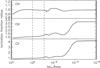 |
Fig. 1 Ratios of ionization fractions resulting from our former and our new model atom, as a function of τRoss, for model D45. The major changes appear for C II and C III ions in the outer wind. The dashed lines enclose the typical line-forming region of optical photospheric lines. |
3.1 Dielectronic recombination
One advantage of testing our carbon description is the availability of two independent codes in our scientific group (FASTWIND and WM-BASIC), which can be used to calculate the same atmospheric models but employing different atomic models. A comparison of the carbon ionization stratification then, for a set of models calculated with FASTWIND and WM-BASIC, gives a quick overview about differences between our results and former work (see Pauldrach et al. 1994, 2001).
In this spirit, we calculated all grid models described in Table 2 also with WM-BASIC. After comparing these models with corresponding FASTWIND ones, we find a rather similar run of C IV and C V, both in the stellar photosphere and also in the wind. In contrast, C II and C III displayed a recurrent difference for all the models: in the wind part, our results lay consistently one or two dex below the outcome from WM-BASIC.
Though this finding does not allow for premature conclusions (at least at this stage, we do not know what is the better description), it nevertheless caught our attention, especially since the same discrepancy had been found for a wide range of temperatures. We thus recalculated the FASTWIND models, but this time using the complete WM-BASIC dataset for carbon. Comparing with our initial models, we found the same difference in C II and C III as described in the previous paragraph. Thus the differences need to be attributed to the different datasets and not to the different atmospheric models, and we set out to compare both datasets in detail.
In the end, we identified the origin of the discrepancy within the radiative bound-free transitions, where each of both datasets describes these transitions differently. While within our new model atom we have used an implicit method to define the dielectronic recombination (henceforth DR11) data within the photoionization cross-sections, the WM-BASIC database adopts an explicit method. Both methods are implemented into FASTWIND: within the implicit method, the resonances appear “naturally” in the photoionization cross-sections (from OPACITY Project data, Cunto & Mendoza 1992), whereas the explicit method considers explicitly the stabilizing transitions from autoionizing levels together with the resonance-free cross-sections. As an example, Fig. 2 displays the data available from the OPACITY Project (black line) with the numerous complex resonances for the ground state of C III, together with the Seaton (1958) approximation using data from WM-BASIC (red line), to which the stabilizing transitions (data input: frequencies and oscillator strengths) would need to be added.
For further details, and advantages and disadvantages of both methods, we refer to Hillier & Miller (1998) and Rivero González et al. (2011). The important point with respect to this work is the following: since in the explicit method one defines each stabilizing transition by corresponding data, we have the possibility to remove any of those transitions by setting the corresponding oscillator strengths to a very low value.
Figure 3 shows the ionization fraction of different carbon ions in the atmosphere, for model D45 (see Table 2). We calculated three different models, where only the bound-free dataset for carbon was changed, leaving all other data at their original value, defined by our new carbon model atom. In the first model, we used the implicit method with bound-free cross-sections from OPACITY Project data, in the second we used corresponding WM-BASIC data (explicit method), and in the third model we discarded the DR-processes in the WM-BASIC data, that is, we used only the resonance-free cross-sections by excluding all stabilizing transitions.
As displayed in Fig. 3, the effect of DR is irrelevant or marginal in the stellar photosphere, where due to the high temperatures and densities the “normal” ionization/recombination processes dominate. In the wind part, the impact of DR remains irrelevant for C IV, but becomes crucial for a precise description of C III. In the case of C II, the difference is mostly a consequenceof changes in C III: without DR, less ions are recombining from C IV to C III, and thus also from C III to C II, due to the lower population. Thus, the differences seen in C III are reproduced in C II, whether DR is present or not. Since CIV is the main ionization stage, the slight increase in its ionization fraction (without DR) is almost invisible.
All models described in Table 2 produce the same effect for C III and C II when DR data are removed. Here we have concentrated on model D45, since for this model we already investigated the effect of DR on the ionization of oxygen in a previous study (Carneiro et al. 2016).
We also investigated which transitions (regarding their lower levels – C III) are responsible for such a change in the wind ionization. It turned out that almost all of the first 40 states are involved, but that levels C3_19, C3_29, and C3_30 (for configuration and term designation, see Table A.2) are responsible for already half of the total effect, where these levels ionize to the second state of C IV.
As shown in Figs. 3 and 5 (see next section), a different treatment of DR can affect the ionization balance of C II and C III in the line-forming region of corresponding optical lines, particularly if this region extends into the wind. Even if such impact is expected to be weak, it should be visible in the synthetic profiles. To see a clear-cut effect, we will concentrate on our (cooler) model D35, where the C II/III lines are certainly visible. Figure 4 compares such lines arising from models calculated with our three different approaches for DR as discussed above (same color-coding as in Fig. 3).
In general, the omission of DR leads to more, while the explicit method leads to less absorption, and our current description lies in between (slightly closer to the non-DR profiles). For most lines, the differences are weak (roughly at the 5 to 10% level at the core), except for C III 4665 (roughly 20%) and C III 5696. The impact of DR on the latter has been already explored by Martins et al. (2012) for a similar model, however with a much lower log g, which turns the line into emission (see also Fig. 6 for a similar behavior in our models). Qualitatively, the effect displayed by both studies is very similar: a larger strength of the stabilizing transitions or resonances leads to more line emission, while reducing these quantities (until a final omission) leads to more absorption.
In conclusion, DR will have no big impact on our and forthcoming spectroscopic analyses, except for C III 5696, which is also affected by other processes such as X-ray emission. For UV-lines that may form throughout the complete atmosphere, however, a realistic description of DR is essential, not only to obtain a fair representation of the observations, but also to achieve consistency with the optical regime.
Finally, we note that also the models calculated with WM-BASIC show the same reaction when DR is excluded (with respect to all or individual stabilizing transitions). We conclude that the two codes independently show a lower degree of C II and C III, once DR is neglected. On the other hand, when actually accounting for DR, the detected differences can be attributed to different strengths of the stabilizing transitions or resonances, where according to our tests all recombiningstates are relevant, though specific transitions (see above) have a particularly strong impact. As a final test onthis issue, we explicitly compared the strengths for the latter transitions (see also Rivero González et al. 2011, Sect. A3), finding a discrepancy of roughly a factor of two (with WM-BASIC data providing larger values).
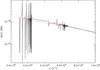 |
Fig. 2 Bound-free cross-section of the C III ground state including resonances (from OPACITY Project, used in our new model atom, black line), and the resonance-free data (from WM-BASIC, red line). |
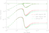 |
Fig. 3 Ionization fractions of carbon ions, as a function of τRoss, for model D45. Note the impact of DR onto C II and C III in the wind region. The dashed lines enclose the typical line-forming region of optical photospheric lines. For details, see text. |
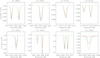 |
Fig. 4 Impact of dielectronic recombination on C II/III lines, for our D35 model (same color-coding as in Fig. 3). The displayed lines are those which are the most influenced ones within our complete set, all others show basically no reaction. Each color represents a different treatment of DR. See text. |
3.2 Further comparison with WM-BASIC
Once the importance of DR in transitions from C IV to C III and its indirect impact on C II has been understood, we can continue in our comparison between FASTWIND and WM-BASIC results.
We remind the reader that both codes are completely independent (except that FASTWIND uses WM-BASIC data for the background elements, i.e., for all elements different from H, He, and C in the case considered here), and use different methods and assumptions. In addition to the different treatment of metal-line blocking, WM-BASIC calculates the velocity field from a consistent hydrodynamic approach, leading to certain differences particularly in the transonic region. Furthermore, while WM-BASIC uses the Sobolev approximation for all line transitions and depths, FASTWIND uses a comoving-frame transport for the transitions from explicit elements and for the strongest lines from the background ones. As we have already mentioned, this can lead to significant discrepancies for those lines that are formed in the region between the quasi-static photosphere and the onset of the wind.
Figure 5 displays the comparison of ionization fractions for carbon ions in the photosphere and wind (as a function of τRoss) for our S45 model (see Table 2). Red lines represent the carbon ionization stratification as derived by WM-BASIC, black lines show the FASTWIND solution using our new model atom, and blue lines display FASTWIND models, where the carbon bound-free transitions including DR are calculated using the explicit method with WM-BASIC data.
For this grid model, C III and C IV (the main ionization stage in the wind) are of major relevance regarding a carbon line diagnostics, though we also display C II (irrelevant at this Teff) and C V, approximated by only one ground-state level in our atomic model. Within the photosphere, differences become visible at certain depths, mostly because of deviations in the density, and due to differences in the line transfer method (see above). In the wind, the standard FASTWIND and the WM-BASIC solution disagree, not only for S45, but also the other grid-models. These differences have been already described in Sect. 3.1, and are due to the different description of DR. When we then manipulated our new model atom to use the bound-free data from WM-BASIC with their larger strengths for the stabilizing transitions, we indeed see much more similar fractions in the outer wind, except for C V, which remains unaffected by DR, since it is insignificant for the C IV/C V balance.
In conclusion, we find a reasonable agreement between results from FASTWIND and WM-BASIC in the photosphere (at least for C III/IV/V). The differences apparent in the wind are due to the fact that the stabilizing transitions in WM-BASIC are larger (or considerably larger for specific transitions) than implied by the resonances provided by the OPACITY Project data. Since we are no experts in this field, we cannot judge which data set is the more realistic one, but until further evidence becomes available we prefer to use the OPACITY Project data, since they are well documented, tested, and applied within a variety of codes and studies.
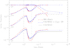 |
Fig. 5 Ionization fraction of carbon ions, as a function of τRoss, for the S45 model, as calculated by WM-BASIC and FASTWIND using different approaches for DR. The dashed lines enclose the typical line-forming region of optical photospheric lines. For details, see text. |
3.3 Optical carbon lines – dependence on stellar parameters
The typical precision of a spectral analysis of massive stars using H/He lines is on the order of ±1.5 kK in effective temperatureand ±0.1 dex in log g (e.g., Repolust et al. 2004). Since we aim for a NLTE carbon abundance determination by line profile fitting, we need to test the sensitivity of our set of strategic lines to a variation of these parameters.
Due to the distinct complexity in each line formation process, almost each of the carbon lines will react differently. Figure 6 (and analogous figures) displays one spectral line per each carbon ion in each of the three columns. The first column shows C II 5145, the middle column C III 5696, and the third one C IV 5801. These lines have been chosen because they are strong (highlighted in Table 1), often discussed in the literature (e.g., Nieva & Przybilla 2008 or Daflon et al. 2004), and visible in different temperature ranges (see Figs. 9–14).
In each panel of Fig. 6, the black profiles refer to model D35. In the upper panels, red profiles correspond to the same model, however with Teff increased by 1.5 kK, while the green profiles, in turn, correspond to a Teff reduced by 1.5 kK. Thus, we are able to study the variation of important carbon lines within the typical uncertainty of Teff. Moreover, the upper panels also display profiles corresponding to model D35, but now with a mass-loss rate (Ṁ) reduced by a factor of three, to estimate the impact of variations in this parameter. The effect of this reduction becomes most obvious for supergiant models (as for example displayed in Fig. 7). In the lower panels, finally, we study the reaction to variations in log g (±0.2 dex).
As shown in the upper left panel, the decrease of temperature leads to a deeper C II absorption, while rising Teff results in a shallower C II profile. This effect is easily understood: lower temperatures increase the fraction of low ionized stages, while higher temperatures favor the presence of higher ions, in this case C IV. From the lower left panel, we see that for the C II profile a decrease of log g leads to a shallower line (less recombination), while the opposite is seen once log g increases (red line).
The panels on the right present the reversed effects for C IV, as expected. For C III 5696 (middle panel), on the other hand, the behavior is quite complex, and has been explored comprehensively by Martins & Hillier (2012). Briefly, the strength of C III 5696 depends critically on the UV C III lines at 386, 574, and 884 Å, because these lines control the population of the lower and upper levels of specific optical C III lines including C III 5696. Indeed, we find a very sensitive reaction of this line on small variations in Teff (upper middle panel), and a similar effect when varying log g (lower middle panel). Without going into further details, during our tests we were able to reproduce all basic effects described by Martins & Hillier (2012), both regarding C III 5696, and also for the triplet C III 4647-50-51.
The consequences of a reduction in Ṁ are clearly seen in the corresponding ionization fractions, where our D35 model with lower Ṁ displays less C II and C III (less recombination) in the wind (~1 dex). Though these differences do not affect the line profiles in a notable way, the weak effect seen in the middle and right panel indicates that these lines are not completely photospheric.
Figure 7 displays a similar study on the reaction of specific carbon lines, now for the supergiant model S35. Since for supergiants the C II lines are already very weak or absent in this temperature range, we display another important C III line instead of the C II profile. Indeed, C III 4068-70 behave similarly to what has been discussed for the C II line in the previous figure. C III 5696 (the one with complex formation) is now in emission, for all cases shown, and C IV 5801 starts to display a P-Cygni shape. For this specific model, a reduction of log g by 0.2 dex brings the model very close to the Eddington limit (Γe ≈ 0.77 already for a pure Thomson scattering opacity). The corresponding stratification becomes very uncertain, and we refrain from displaying corresponding profiles.
Since a supergiant (model) exhibits a denser wind than a dwarf, the effects of a mass-loss reduction on the line profiles are more obvious than for model D35. Also here, the model with reduced Ṁ displays a lower fraction of C II and C III in the outer wind. Particularly in the line forming region, however, the ionization fractions of all ions become larger. The leftmost panel shows that a reduction of Ṁ leads to a stronger C III 4068-70 absorption, where the effect is even more pronounced than the effect of the temperature reduction or the gravity increase. In the middle panel, the effect is similar, now acting on an emission profile. Again, we see a larger response than on the temperature decrease, which is also true for the right panel. Additionally, the P-Cygni shape almost vanishes, due to the inward shift of the line-forming region.
Finally, and for completeness, Appendix B provides the same analysis, now for the cooler and hotter dwarf and supergiant models at 30 kK and 40 kK, and for partly lower changes in Teff and log g. In addition to mostly similar reactions as described above, we note the different reaction of C III 5696 on the variation of log g in the supergiant models: while for largest log g both S30 and S35 yield the lowest emission, this behavior switches for S40, where the highest log g results in the largest emission. Again, this nonmonotonic behavior is due to the complex formation process of this line. Additionally, Fig. B.5 displays the reaction of our complete set of lines on a change of stellar parameters.
Overall, the tests performed in the section indicate that most of our strategic carbon lines are quite sensitive to comparatively small variations of the stellar parameters, variations that are within the precision of typical atmospheric analysis of massive stars performed by means of H and He. Moreover, some of them depend on UV transitions (as, e.g., C III 5696). Since X-ray emission affects UV lines, we need to check which of our optical lines indirectly depend on the strength of the X-ray emission (see Sect. 4.4).
By the end of this test, we are able to conclude that even in those cases where the stellar parameters are “known” from a H/He analysis, a small model grid needs to be calculated for each stellar spectrum which should be analyzed with respect to carbon. This grid needs to be centered at the (previously) derived Teff and log g values found from H/He alone, and should extend these values in the ranges considered above12. One of these models should then allow for a plausible fit for the majority of our C II/III/IV lines (and not destroy the H/He fit quality), for a unique abundance and micro-turbulent velocity, vturb.
Finally, we emphasize that all the tests discussed thus far only give a first impression on the capabilities of our new model atom. The quality and reliability of these results can be estimated only via a detailed comparison with observations, for a large range of stellar parameters. A first step into this direction is the main topic of the next section.
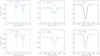 |
Fig. 6 C II 5145, C III 5696, and C IV 5801 line profiles for model D35 (black lines) and similar models with relatively small changes in effective temperature (Teff) and gravity (log g). Upper panels: red lines correspond to a D35 model with Teff increased by 1500 K, the green lines to a model with Teff decreased by the same value, while the blue lines display the reaction to a decrease of Ṁ by a factor of three. Lower panels: red lines correspond to a D35 model with log g increased by 0.2 dex, and the green lines with log g decreased by 0.2 dex. |
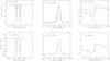 |
Fig. 7 As Fig. 6, but for model S35. Since the C II lines are absent in such a model, we display another strategic line for this temperature range, C III 4068-70. We note that log g has only been varied by +0.2 dex (red profiles) in the lower panel. See text for details. |
4 First comparison with observed carbon spectra
4.1 Basic considerations
For our comparison with observations and a first analysis, we used six spectra of presumably single Galactic O-type stars in different temperature ranges. Because of the weakness of most lines and the blending problem, rotational broadening is of major concern for a meaningful comparison of synthetic and observed spectra. Usually, hot massive stars are fast rotators (e.g., Simón-Díaz & Herrero 2014), and any large value of v sin i (particularly in combination with a significant extra-broadening due to “macroturbulence”, vmac) makes the majority of carbon lines very shallow or even too shallow to be identified. Thus, we restricted ourselves to comparatively slow rotators.
Our subsample comprises three dwarf and three supergiant O stars, observed with different instruments. However, all spectra cover the wavelength range relevant for this work. As in our previous tests, we cover the same interval of temperature, from ~30 kK to ~50 kK. Thus, we expect to analyze C II /C III for the coldest stars, while the hotter stars provide an opportunity to check our precision in reproducing C III and C IV lines.
The reduced and normalized13 spectra were kindly provided and extracted from the work by Holgado et al. (2018). In this work, the parameters of a large sample of Galactic O-stars were obtained by quantitative H/He spectroscopy using FASTWIND, where we have already summarized some observational details in Sect. 2.5.
For our subsample, we double-checked their results by an independent FASTWIND analysis (fitting by-eye, contrasted to the semi-automatic fitting method applied by Holgado et al. (2018) using precalculated grids of synthetic spectra and the GBAT-tool, Simón-Díaz et al. 2011), and found an agreement of photospheric and wind parameters (in particular, Teff, log g, log Q – see below –, v sin i, and vmac) on a 1 − σ level. We also checked the radial velocities using the H/He lines, and confirmed the values provided byHolgado et al. (2018) for almost all subsample stars (differences less than 10 km s−1), except for CygOB2-7, where we found a difference of 20 km s−1.
Holgado et al. (2018) estimated the wind-strength parameter,  (e.g., Puls et al. 2005) for each star in their sample, though they did not provide individual values for Ṁ, R*, and v∞ as required for the FASTWIND input. We estimated these quantities using their Q-values, an estimate of v∞ (via vesc, using log g, R*, and Teff, see Kudritzki & Puls 2000), and an adopted stellar radius, R*, following the Martins et al. (2005) calibration between spectral type and radius.
As shown in Sect. 3.3, the uncertainties (error bars) on the stellar and wind parameters derived from H/He alone are quite large when accounting for the sensitivity of the carbon lines. Therefore, after having defined a first guess of these parameters, there is still a sufficiently large interval in Teff and log g to vary those parameters and to find the best matching carbon ionization balance (in those cases where more than one ion is present), while preserving the overall fit-quality of the H/He lines. To this end, we varied Teff and log g inside intervals of ±1,000 K and ±0.1 dex, respectively, centered at the initial values derived by Holgado et al. (2018).
Figure 8 displays the Teff-sensitivity of important diagnostic carbon lines (right two columns) in comparison to H/He lines (left two columns). For this example, we have chosen our coldest dwarf object (HD 36512, O9.7V), where further details will be discussed in the next section. On the figure we plot the initial model calculated with the values obtained by Holgado et al. (2018). Obviously, this model has much stronger C II and weaker C IV than the observations. Evidently, the effective temperature needs to be adjusted, even though it reproduces well the H/He profiles. In this case, C III does not display a remarkable sensitivity, since it is the main ion throughout the atmosphere.
All colored lines represent models with the same log g, v sin i, vmac, Q, and [C/H] = log C/H + 12 (by number) values (see Table 3), but with different Teff. We note that [C/H] had already been reduced by 0.2 dex with respect to solar abundance (see below), to obtain reasonable fits. The color coding is described in the figure legend. All models reproduce equally well the H/He lines, though the variation in carbon is significant. We conclude that in this case, the Teff = 33.8 kK profiles are closest to observations, and that it is possible to represent all three ionization stages in parallel with the adopted abundance. We note that here we did not haveto change log g.
As we have double-checked all stellar and wind-parameters (but varied Teff and log g to improve on the carbon ionization balance), and these parameters turned out to be sufficient to reproduce the H/He and C profiles, we have not performed an independent error analysis, and refer to the values suggested by Holgado et al. (2018).
Regarding the carbon abundances, we used, at least in principle, all the lines from our set as indicators, through a by-eye fit, but lines which eventually displayed an unexpected behavior (e.g., too much emission), were discarded. In this context, we remind on the complexity of spectroscopic analyses for hot stars, compared to cooler ones. Due to the presence of, for example, strong NLTE effects, winds, and possibly clumping, which might “contaminate” individual lines, our goal is to obtain a best compromise solution from lines of the available carbon ions, and to constrain the carbon abundance within a reasonable range. In our opinion, it is better to obtain such a compromise solution for as many lines and ions as possible, instead of aiming at perfect fits for few lines only. We note here that deviations between synthetic and observed profiles are not as strongly related to inadequate atomic data as it is the case in cooler stars, but also depend on all the other uncertainties mentioned above.
The above compromise solution was achieved as follows. At first, we calculated a model with solar carbon abundance14, and two more models with this abundance varied by ±0.2 dex. This first step allowed us to identify if, in general, the visible carbon lines agree better with a solar, supersolar, or subsolar abundance. In a second step, we fine-tuned Teff and log g as outlined above. To specify the final carbon abundances and their uncertainties (i.e., the above range), we used the first estimate of [C/H], and calculated, if necessary, one further model, with [C/H] enhanced or decreased by 0.2 dex (in dependence of the result from step one). In case – this was not necessary for our sample –, this process needs to be repeated, and the final range should comprise reasonable fits for all lines of our set. As quoted abundance then, we adopt the center of this range. The chosen interval of ±0.2 dex allows us also to obtain a rough estimate on the associated uncertainty. If a step of ±0.2 dex was too large, the process was repeated with abundances increased or decreased by only 0.1 dex, as indicated by the line fits, Figs. 9–14.
Table 3 summarizes the final values derived from our fits to the optical H/He15 and C-lines, for all objects considered. The table includes two values for Teff and log g, corresponding to the initial (from Holgado et al. 2018, partly priv. comm.) and updated values.
4.2 Details on individual spectra
In the following, each of the spectra and corresponding fits will be discussed in fair detail. Figures 9–14 present the observed spectra and our best compromise solution, corresponding to the parameters as given in Table 3. The colors in the figure refer to a carbon abundance increased and decreased by 0.2 dex (seefigure caption). These profiles not only provide us with an estimate on the error of our finally derived abundance (see above), but also allow us to identify which of the lines are more or less sensitive to abundance variations.
The source HD36512 (υ Ori) is an O9.7V slow rotator, observed with the HERMES spectrograph (see Fig. 9). We fitted the H/He and C lines with a temperature of 33.8 kK and log g = 4.02. The obtained stellar parameters agree well with the values derived by Holgado et al. (2018). This is one of the stars where all the carbon ions have well-defined observable lines.
Our synthetic spectra reproduce quite well the C II and C IV lines. C II 4637 is absent (O II 4638.9 dominates the range), as well as C II 5133. The region around C II 6578 is badly normalized, but even with a renormalization the line would still be reproduced inside the adopted range. For C III, most lines are reproduced, except for C III 5272 and the C III4068-70 doublet, which always seems to indicate a lower carbon abundance than inferred from the other lines. At least for this object, the discrepancy seems to be stronger for the C III 4068 component than for its λ4070 Å companion, but we note that the blue component is strongly influenced by O II 4069.8. Finally, C III 6744 is too weak in comparison to our models.
As a compromise, we derive a carbon abundance of [C/H] = 8.25 dex, which brings most carbon lines into agreement. Few of our lines point to slightly higher abundances (e.g., C III 4056-5696-8500), and therefore we estimate a range of ±0.22 dex for the involved uncertainties. This spectrum is an example for an ideal scenario, mainly due to the low rotation rate (v sin i = 13 km s−1) and low macroturbulence (vmac = 33 km s−1), where our carbon model produces very satisfactory results. Martins et al. (2015a) have analyzed this star as well, and they derived, in addition to rather similar stellar parameters, also a carbon abundance ([C/H] = 8.38 ± 0.15) that is consistent with our result.
The star HD303311 is an O6V star with a projected rotational velocity of 47 km s−1, and a macroturbulence of 61 km s−1 (Fig. 10). The spectrum has been collected with the FEROS spectrograph. We obtained a final value of 41.2 kK for the temperature and of 4.01 for log g, both slightly adjusted after the reproduction of the H/He lines to the best agreement with the different carbon lines. At this temperature (and rotational velocity), the lines of C II already vanish, and the C III profiles are weak, while the C IV lines are still easily detectable. In this case, however, C IV is the main ionization stage, and therefore not as sensitive to variations in the stellar parameters as the other carbon ions16. Our synthetic lines show a good reproduction of the C III lines. Once more, C III 4068-70 indicate a lower abundance when compared to the other C III profiles, however the difference is not larger than 0.2 dex. C III 6731 surprisingly displays an emission profile. There seems to be a disagreement between the carbon abundance indicated by the C III and C IV lines. Both C IV profiles point to a higher [C/H]-value, but again the difference is not larger than 0.22 dex. The best compromise was found for a carbon abundance of 8.33 ± 0.25 dex.
The star HD93128 is an O3.5V star rotating with 58 km s−1, a macroturbulence of 56 km s−1, and was observed with the FEROS spectrograph (Fig. 11). The temperature has been decreased by 300 K from the value obtained by the pure H/He analysis, but is still in agreement with the value from Holgado et al. (2018) when considering their 1-σ interval. We used 48.8 kK for the temperature, and 4.09 for log g. In this temperature regime, some weak signs of C III might be seen only by chance. Furthermore, also the C IV-analysis becomes difficult, because the lines start to switch from absorption to emission, and a distinction from the continuum is harder in this case. Additionally, He II 5800 broadens C IV 5801.
Nevertheless, at least a rough estimate for the carbon abundance might be provided, mostly from C IV. In Fig. 11, we fit the weak sign of C III 4650, and also C IV 5812, and we infer [C/H] ≈ 8.23 dex. Due to the very low number of available lines, we adopt a larger uncertainty in our estimate, ±0.3 dex.
The star HD188209 is an O9.5Iab star with v sin i of 54 km s−1, a macroturbulence of 93 km s−1, and has been observed with the HERMES spectrograph (Fig. 12). The temperature and gravity obtained from fitting the H/He lines agree well with the stellar parameters derived from Holgado et al. (2018; Δ Teff = 200 K), and were used in our final model including the carbon line diagnostics (Teff = 30.3 kK, log g = 3.03). C III and C IV lines are easily identified, while C II lines are not present in this case, except a subtle sign of C II 4267, which is well reproduced by our synthetic profile. The C III and C IV lines, even being weak, are well described by the synthetic profiles, and the discrepancy of C III 4068-70 is somewhat lower than found in the cases above. Here, C III 4650 shows the largest deviations. We note also the poor normalization around C III 4070 and C III 5800. Our final solution for [C/H] is 8.23 dex, and due to nonfitting lines we increase our error budget to ±0.25 dex. Also this star has been analyzed by Martins et al. (2015a). Again, the stellar parameters are in very good agreement, but here the derived carbon abundance ([C/H] = 7.85 ± 0.3 dex) only marginally overlaps with our value within the quoted error intervals.
The star HD169582 (O6Ia) rotates with v sin i = 66 km s−1, has a macroturbulence of 97 km s−1, and was observed with the FEROS spectrograph (Fig. 13). A temperature of 39 kK and log g of 3.7 were used to synthesize the carbon lines. Both values agree with the ones suggested by Holgado et al. (2018). C III is very weak and almost invisible, and only the C IV profiles are easily visible. Firm conclusions about C III are not possible, though we note that the synthetic lines indicate a weak signal. A carbon abundance of 8.53 dex gives a fair compromise for the C III/C IV lines, though C IV seems to indicate a slightly higher abundance than C III. We note however that none of the lines requires an abundance outside the ±0.2 dex interval.
The star CygOB2-7 is one of the few O3I stars in the Milky Way. Its spectrum (Fig. 14) has been recorded by the FIES-spectrograph, and extends “only” to a maximum of 7000 Å, so that C III 8500 is not available. We note that this spectrum has the lowest S/N within our subsample. A Teff of 51 kK and a log g of 4.09 (together with v sin i = 75 km s−1 and an astonishingly low vmac = 10 km s−1) enable a satisfactory fit to the H/He lines. In this temperature regime, only C IV is visible, switching from absorption to emission (at least at the given Ṁ). This behavior complicates the reproduction of the C IV profiles, and forbids any stringent conclusions. Especially in this case, one would also need to analyze the UV spectrum. If we believe in the ionization equilibrium and the mass-loss rate, we derive an abundance around [C/H] ≈ 8.0, which would be the lowest value in our sample. From the fit quality and since we have to firmly rely on our theoretical models (no constraint on the ionization equilibrium), we adopt an asymmetric error interval, − 0.4 and + 0.3 dex.
As mentioned in Sect. 2.3, one of the “classical” problems in carbon spectroscopy is an inconsistent abundance implied by C II 4267 and C II 6578-82. Once more, we remind on the work by Nieva & Przybilla (2006) who thoroughly investigated and solved this problem for a set of stars cooler (with stronger C II lines) than the ones considered in this work. These C II lines are clearly visible and well reproduced with the same value of [C/H] in our coldest dwarf, HD 36512. This provides strong evidence that our present data are sufficient to overcome this issue. Also for our coldest supergiant, HD 188209, C II 4267 is present and well reproduced. On the other hand, C II 6578-82 is absent, and thus no further conclusions can be asserted.
We finish this section by noting that part of the problems in fitting certain lines might be related to our assumption of a smooth wind (and neglecting X-ray effects, but see Sect. 4.4). Effects due to clumping etc. will be investigated in a forthcoming paper. In this regard, the abundance estimates presented in Table 3 should be taken with caution: contrasted to cooler-type stars where the synthetic profiles depend primarily on the precision of atomic data, for early type stars with winds much more uncertainties have to be accounted for (and approximated in a reasonable way).
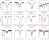 |
Fig. 8 Fine-tuning of stellar parameters (here, Teff), for the case of HD 36512 (O9.7V). The stellar parameters initially estimated from the H/He lines (green) still need some additional fine tuning, since some of the carbon lines are much more sensitive to small changes than H/He. The color coding for Teff is as follows. Green: 33 kK (see Holgado et al. 2018), blue: 33.6 kK, turquoise: 33.8 kK, and red: 34 kK (the latter displaying too much C IV). |
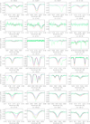 |
Fig. 9 Observed carbon spectrum of HD 36512 (O9.7V, green), and synthetic lines (black), calculated with [C/H] = 8.25 dex. The red and blue profiles have been calculated with an abundance increased and decreased by 0.2 dex, respectively. |
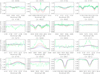 |
Fig. 10 As Fig. 9, but for HD 303311 (O6V), and a carbon abundance of 8.33 dex. The optical C II lines are not visible, and thus not displayed. |
4.3 Which lines to use?
After our first analysis, we acquired enough experience to judge in which lines to “trust” when deriving carbon abundances.In Table 1, we provided a comprehensive list, comprising many more lines than previously studied, which are strong enough to be easily identified in different temperature ranges. Instead of describing which of these lines are the most useful, we summarize which may be discarded, since this results in a shorter list.
For C II, the range around C II 4637 is dominated by O II 4638, and therefore the carbon lines are barely visible. C II 5648-62 are isolated lines which can be important, but are not visible in the range of spectral types studied in this work (O9-O3). The same is true for C II 6461. The lines at 5139 and 6151 Å are formed by transitions with low oscillator strength, and might be too weak for a meaningful spectral diagnostics. Excluding these lines, we were able to identify all the other C II lines as listed in Table 1 in the observed spectra (for the cooler spectral types), and to use them within our analysis.
The largest number of lines is provided by C III, when considering the complete O-star range. Particularly, all the listed lines are visible in the coldest dwarf of our sample (Fig. 9). C III 4068-70 always (i.e., for the complete temperature range) pointto lower abundances (compared to the majority of other lines), and it might be that particularly the λ4068 Å component is either mistreated by our approach, or that there is a problem with its oscillator strength. The lines at 4650 and 5696 Å always deserve special attention, because of their complex formation process, even though we were able to reproduce these lines well in the majority of cases studied here. The lines at 5826, 6731, and 6744 Å are also good diagnostics, but vanish quickly for spectral types earlierthan O9.
For C IV, basically four lines are available in the optical range, but the ones at 5016-18 Å are outshone by He I 5015. Therefore, and to our knowledge, all optical C IV analysis performed until to-date have concentrated on C IV 5801-12, and this most likely will not change in future.
Discarding the lines quoted above, we end up with a list of 27 lines from C II/III/IV that are useful for determining reliable carbon abundances, indicated in boldface in Table 1.
4.4 Impact of X-rays
In a previous paper (Carneiro et al. 2016), we already discussed the impact of X-ray radiation on the ionization stratification of different ions, including carbon. Here we investigate which of the optical lines are affected by emission from wind-embedded shocks, and how intense the X-ray radiation must be to have a relevant impact on the lines. As pointed out before, purely photospheric lines without any connection to UV-transitions should not be affected by X-rays, at least in principle. However, lines that are purely photospheric for thin winds are partly formed in the wind when the mass-loss rate becomes larger, and also the lower boundary of the X-ray emitting volume is important in controlling how much X-ray/EUV radiation can reach the photosphere. Even more, since the X-ray luminosity scales with the mass-loss rate (or, equivalently, with the stellar luminosity, e.g., Owocki et al. 2013), carbon lines in high-luminosity objects might become affected by X-ray emission even when they are not connected with UV-transitions.
The main idea of our study is to adopt the strongest possible (and plausible) shock radiation, and to check which lines will change. For the present analysis, few parameters will describe the shock radiation in each model, leaving the others at their default (see Carneiro et al. 2016 for details). These are the X-ray filling factor, fx, which is related to (but not the same as) the (volume) fraction of X-ray emitting material, and the maximum shock temperature,  . Both are set here to the maximum values used in our previous analysis: fx = 0.05, and
  K. Besides this “maximum-model”, we checked also the impact for intermediate values of the X-rays parameters (fx = 0.03, and
  K). Another important parameter is the onset of X-ray emission, Rmin. Guided by theoretical models on the line-instability and/or by constraints from X-ray line diagnostics, Rmin is conventionally adopted as ~1.5 R* (e.g., Hillier et al. 1993, Feldmeier et al. 1997, Cohen et al. 2014). Since we want to maximize any possible effect from the X-ray radiation, we set Rmin = 1.2 R*.
Before turning to the general results of our simulation, we remind on the sensitivity of C III 5696 and C III 4647-50-51, showing significant changes in strength and shape for small variations of local conditions in the 30-40 kK regime (see Fig. 6 and Martins et al. 2012 for a thorough analysis). As expected (both transitions are connected to UV resonance lines), these lines are indeed sensitive to the presence of X-rays.
After checking all lines tabulated in Table 1 regarding a potential influence of X-ray emission, no changes were found for the 30 kK and 35 kK dwarf and supergiant models. Even for C II in these coolest models, no impact was seen, which indicates that either the X-ray radiation is still too weak (because of low mass-loss rates), or that it cannot reach the photosphere.
From 40 kK on, however, the situation changes. In almost all cases, only the C IV lines become weaker, and by a considerable amount for supergiants (see below) and our D50 model. Most C III lines become only marginally stronger or weaker, if at all, and the only more significant reaction is found for the strongly UV-influenced C III 4647-50-51 and C III 5696 lines. When including shock radiation, their strength increases at hottest temperature(s), comparable to an increase in carbon abundance of 0.1 dex.
Beyond 40 kK, the ionization fraction of C IV decreases (both in the line-forming region and the wind) when the X-ray emission is included. For dwarfs, the corresponding line-strengths of C IV 5801-5811 (in emission) decrease in parallel, by an amount still weaker than 0.1 dex in [C/H].
For the supergiants, this effect becomes stronger in the 40 to 45 kK regime, while for S50, finally, the impact of X-rays on the C IV lines becomes weak again, presumably because in this temperature range the stellar radiation field dominates in controlling the ionization equilibrium. We note that for the D50 dwarf model the changes remain considerable though.
In Fig. 15, we detail this behavior, for our S40 model, where the effect is strongest. On the figure we plot a model without X-rays, a model with intermediate shock radiation, and the model with our strongest X-ray emission. The dotted profiles give an impression of a corresponding decrease in carbon abundance which would be necessary to mimic the X-ray effect, which is 0.3 and 0.6 dex, respectively. The other way round, for stars that have been analyzed without X-rays but exhibit a strong X-ray radiation field, the originally derived carbon abundance might need to be increased by such an amount to compensate for the missing X-ray field. Our investigation clearly indicates that X-rays may be important for the C IV analysis of supergiant stars with temperatures around 40 to 45 kK (e.g., the prototypical ζ Pup) and for (very) hot dwarfs, in particular if no lines from other carbon ions are present.
In summary, the changes are marginal for not too hot dwarfs, and affect only a few C III lines (the triplet at 4647-50-51, the doublet at 4663-65, and C III 4186, 5272, 5696, 5826, 6744, 8500 Å) which might be used with a lower weight in abundance analysis.
In contrast, and at least for supergiants in the range between 40 to 45 kK, various lines become substantially modified when accounting for strong emission from wind-embedded shocks, in particular the two C III lines that are strongly coupled to the UV, and the C IV lines. The potential differences in abundances derived from these lines (~0.1 dex from C III 4647-50-51 and C III 5696, and ~0.3 to 0.6 dex from C IV 5801-5811) may complicate the analysis considerably, and we conclude that the carbon analysis of supergiants earlier than O7 should include X-ray radiation using typical default values, as already standard for CMFGEN modeling. We note (i) that this problem might have also affected our analysis of HD 169582, and (ii) that X-rays might need to be considered in the analysis of (very) hot dwarfs as well, due to their impact on C IV.
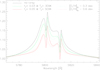 |
Fig. 15 Impact of X-ray radiation on the C IV 5801-12 lines, for a supergiant model with Teff = 40 kK (S40). Black: line profiles for the “standard” model without shocks; green: model with an intermediate X-ray strength; red: model with strong X-ray radiation. The dotted profiles refer to alternative, no-shock models with reduced carbon abundance, mimicking the effect of shock radiation. We note that the displayed sensitivity is strongest for the considered lines and parameter range, see text. |
5 Summary and conclusions
In this work, we aimed to enable a reliable carbon spectroscopy by means of our unified NLTE atmosphere code FASTWIND. To this end, we developed a new carbon model atom using high-accuracy data from different databases. The data adopted to describe the radiative and collisional transitions have been cross-checked (with similar data from alternative databases) to ensure their reliability. We implemented an adequate number of levels following certain rules, though additional levels might be required for the analysis of IR-transitions in future studies. In total, we considered 162 LS-coupled levels, more than 1000 radiative, and more than 4000 collisional transitions.
One major issue for this study was a rigorous test of our new model atom. For this purpose, we calculated a sufficiently spaced grid of atmospheric models, to investigate the carbon ionization structure, and to compare with previous results using more simplified model atoms.
Interestingly, dielectronic recombination (DR) turned out to be of major importance for the description of C II and C III in the wind, for almost all temperatures17. When DR isneglected, we find less recombination from C IV to C III, and consequently also less C II. Typical differences amount to 1 dex. Similar results were reproduced with WM-BASIC, though we found an important difference between the underlying data: the strengths of the stabilizing transitions used in WM-BASIC are typically larger (up to a factor of approximately two) than those corresponding to the strengths of the resonances included in the OPACITY Project data we have used, leading to stronger recombination in WM-BASIC models. Even though this potential uncertainty will not affect the majority of optical lines formed in the photosphere, it can be influential in upcoming analysis of UV wind lines. In the end, we preferred to use the OPACITY Project data, for reasons outlined in Sect. 3.1.
Unfortunately, optical carbon lines are rare, and often blended by other lines, which hampers the spectral diagnostics, particularly for large v sin i and/or vmac. Thus, we compiled and selected a maximum set of potential diagnostic lines, including blended ones and also those with a complex formation mechanism controlled by UV transitions (as described by Martins et al. 2012).
Since the majority of metal lines are weak, they are very sensitive to comparatively small variations of stellar parameters, and this is particularly true for carbon lines. A change of ±1000 to 1500 K in effective temperature, or ±0.2 dex in log g, results in considerable changes of line strength. Additionally, some of the lines are also sensitive to Ṁ variations. Mainly in supergiants (and hot dwarfs), due to their dense winds, a decrease in Ṁ by a factor of three produces an effect stronger than a decrease of 1500 K in Teff or an increase of 0.2 dex in log g. Thus one needs to precisely determine Ṁ by reproducing, for example Hα and He II 4686, before aiming at a carbon analysis.
As a first application of our “new” capability to analyze carbon lines by means of FASTWIND, using our newly developed model atom, we investigated the spectra of a sample of six O-type dwarfs and supergiants, kindly provided to us by Holgado et al. (2018). We first convinced ourselves that the stellar and wind parameters derived by Holgado et al. (2018) are reproduced by our own H and He analysis. Thereafter, we varied Teff and log g inside a range where the fit quality of the H/He lines could be preserved (roughly, ±1000 K and ±0.1 dex, respectively), while fitting the carbon lines from different ions in an optimum way, with an (almost) unique abundance in most cases. The finally quoted abundance was taken, if necessary, from the best-compromise solution, and from the reaction of the carbon lines when varying the abundances, we obtained a rough estimate on the corresponding error, typically in the range ±0.2 to ±0.3 dex.
Only for the coolest (O9.7) dwarf, lines from all three ionization stages are present in parallel, and our analysis resulted in a satisfactory reproduction of the ionization balance. In most other stars, only C III and C IV are visible in parallel. For one object with Teff≈ 40 kK (HD 169582), these C III/ IV lines disagree by ~0.2 dex in [C/H], which might be related to the influence from X-ray radiation (see below). The hottest (O3) supergiant, CygOB2-7, displays only C IV, which renders the analysis quite uncertain (and there are only two suitable C IV lines in the optical).
We were, nevertheless, able to derive carbon abundances for all the considered objects, and found in most cases a moderate depletion compared to the solar value by Asplund et al. (2009), except for CygOB2-7, where a larger depletion by 0.4 dex was derived (though more uncertain than the other values). Two of our cool objects had already been analyzed by Martins et al. (2015a). For both of them we confirmed rather similar stellar parameters, but only for one of them (a dwarf) also the carbon abundances are quite similar, while for the other (a supergiant), there is an only marginal overlap within the errors.
To obtain further constraints on the reliability of our new set of synthetic carbon lines, we have to repeat the same exercise in particular for cooler stars, since C II already disappears for Teff ≳ 30 to 35 kK, in dependence of luminosity class.
From our accumulated experience of analyzing basically all optical carbon lines, we finally provided a list of more than 25 lines of different strength and from different ions, which we consider as reliable carbon abundance indicators.
As a first step toward future work, we studied the direct and indirect (via UV-lines) impact of X-ray emission from wind-embedded shocks onto our sample of optical carbon lines, by simulating an X-ray radiation field that is at the upper limit of realistic values.
For the dwarf models, we found an almost negligible impact, except for very hot objects (≳50 kK). In contrast, carbon lines from supergiants with Teff ≈ 35 kK already show changes due to shock radiation, and at 40 to 45 kK the impact of X-rays is strong enough to complicate a reliable abundance measurement. Mostly, the C III lines become stronger (corresponding to an increase of up to 0.1 dex in [C/H]; the largest changes occur in the UV-influenced C III 5696 and C III 4647-50-51), and the C IV lines become weaker (corresponding to a decrease of 0.3 to 0.6 dex in [C/H]). Consequently, it might become more difficult (or even impossible) to find a value of [C/H] which brings different carbon lines into agreement, when strong X-ray emission would be present. Thus we concluded that in the spectral regime earlier than O7 I, it might be necessary to include the impact of X-rays by default (though a deeper understanding of typical X-ray parameters might be required as well). For supergiants with Teff ≳ 50 kK, the X-rays lose their impact, since direct ionization due to the stellar radiation field dominates over Auger-ionization and ionization from the EUV-component of the shock radiation (see Carneiro et al. 2016).
This study has been performed as a first step toward a complete CNO analysis. Particularly the investigation of the ratio N/C vs. N/O (as already begun by Martins et al. 2015a,b) will allow us to derive better constraints on the mixing history and chemical enrichment in massive stars than from a pure nitrogen analysis alone. We intend to continue such work, also by including the information provided by UV carbon lines, and by investigating the impact of wind inhomogeneities, which might play an important role also in the UV range, due to porosity effects and because of affecting the ionization balance in the wind.
Acknowledgements
We thank our anonymous referee for very useful comments and suggestions. L. P. C. gratefully acknowledges support from the Brazilian Coordination for the Improvement of Higher Education Personnel (CAPES), under grant 0964-13-1. Many thanks also to G. Holgado and S. Simón-Díaz for providing us with the optical spectra for six Galactic O-type stars, and to N. Przybilla and M. Urbaneja for their help, material and suggestions to build the carbon model atom. Special thanks to Keith Butler for all his explanations regarding atomic data and corresponding databases.
Appendix A Electronic states of each carbon ion
This section provides a short description of each ion considered in our new carbon model atom, except for C V which is described by the ground level only (see Sect. 2.2). All the next threetables have the same format: the first column displays the label of the level, the second column the electronic configuration of that level, and the third column presents theterm designation. Table A.1 refers to C II, Table A.2 to C III, and Table A.3 to C IV.
C II levels: label, electronic configuration, and term designation.
Appendix B Dependence on stellar parameters
This appendix displays the sensitivity of synthetic carbon spectra from dwarf and supergiant models at 30 and 40 kK, with respect to variations inTeff, log g, and Ṁ. Figures B.1 to B.4 have the same layout as Fig. 6, and refer to Sect. 3.3, where also the corresponding discussion has been provided. For completeness, Fig. B.5 displays the sensitivity with respect to variations inTeff and log g for our complete set of lines, with the same color coding as in Fig. 6.
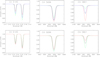 |
Fig. B.1 C II 5145, C III 5696, and C IV 5801 line profiles for model D30 (black lines, see Table 2) and similar models with relatively small changes in effective temperature (Teff) and gravity (log g). Upper panels: red lines correspond to a D30 model with Teff increased by 1000 K, the green lines to a model with Teff decreased by the same value, while the blue lines display the reaction to a decrease of Ṁ by a factor of three. Lower panels: red and green lines correspond to a D30 model with log g increased and decreased by 0.15 dex, respectively. |
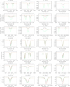 |
Fig. B.5 Carbon line profiles for model D35 (black), and dependence on stellar parameters, for our complete set of lines. The red and green solid line profiles correspond to an increase and decrease by 1500 K in Teff, respectively, whereas the red and green dashed profiles correspond to a variation of +0.2 dex and −0.2 dex in log g. |
The general behavior is similar to the lines already discussed in this appendix and Sect. 3.3, but not identical, due to different formation regions and processes. (We note that C II 5648 is absent for this model.) The major exception is C II 6461, where the emission displayed by the central model is reduced when any kind of variation in Teff or log g is applied. However, the predicted line is so weak that an actual understanding of the actual origin of this behavior is difficult to obtain.
References
- Aggarwal, K. M., & Keenan, F. P. 2004, Phys. Scr., 69, 385 [NASA ADS] [CrossRef] [Google Scholar]
- Allard, N., Artru, M.-C., Lanz, T., & Le Dourneuf, M. 1990, A&AS, 84, 563 [NASA ADS] [Google Scholar]
- Allen, C. W. 1973, Astrophysical quantities, 3rd edn. (London: University of London, Athlone Press) [Google Scholar]
- Asplund, M., Grevesse, N., Sauval, A. J., & Scott, P. 2009, ARA&A, 47, 481 [NASA ADS] [CrossRef] [Google Scholar]
- Bièmont, E. 1977, A&AS, 27, 489 [NASA ADS] [Google Scholar]
- Butler, K., & Giddings, J. R. 1985, Newsl. Anal. Astron. Spectra, 9 [Google Scholar]
- Carneiro, L. P., Puls, J., Sundqvist, J. O., & Hoffmann, T. L. 2016, A&A, 590, A88 [NASA ADS] [CrossRef] [EDP Sciences] [Google Scholar]
- Chiappini, C. 2001, Am. Sci., 89, 506 [NASA ADS] [CrossRef] [Google Scholar]
- Chiappini, C. 2002, Ap&SS, 281, 253 [NASA ADS] [CrossRef] [Google Scholar]
- Cohen, D. H., Wollman, E. E., Leutenegger, M. A., et al. 2014, MNRAS, 439, 908 [NASA ADS] [CrossRef] [Google Scholar]
- Cowley, C. R. 1971, Observatory, 91, 139 [Google Scholar]
- Cunto, W., & Mendoza, C. 1992, Rev. Mex. Astron. Astrofis., 23, 107 [NASA ADS] [Google Scholar]
- Daflon, S., & Cunha, K. 2004, ApJ, 617, 1115 [NASA ADS] [CrossRef] [Google Scholar]
- Daflon, S., Cunha, K., & Becker, S. R. 1999, ApJ, 522, 950 [NASA ADS] [CrossRef] [Google Scholar]
- Daflon, S., Cunha, K., Becker, S. R., & Smith, V. V. 2001a, ApJ, 552, 309 [NASA ADS] [CrossRef] [Google Scholar]
- Daflon, S., Cunha, K., Butler, K., & Smith, V. V. 2001b, ApJ, 563, 325 [NASA ADS] [CrossRef] [Google Scholar]
- Daflon, S., Cunha, K., & Butler, K. 2004, ApJ, 604, 362 [NASA ADS] [CrossRef] [Google Scholar]
- Eissner, W. 1991, J. Phys. IV, 1, C1 [Google Scholar]
- Eissner, W., & Nussbaumer, H. 1969, in Première Réunion de l’Association Européenne de Spectroscopie Atomique N° 42 (Paris-Orsay: Faculté des Sciences) [Google Scholar]
- Feldmeier, A., Kudritzki, R.-P., Palsa, R., Pauldrach, A. W. A., & Puls, J. 1997, A&A, 320, 899 [NASA ADS] [Google Scholar]
- Giddings, J. R. 1981, PhD Thesis, University of London, UK [Google Scholar]
- Glass, R. 1983, Ap&SS, 92, 307 [NASA ADS] [CrossRef] [Google Scholar]
- Gräfener, G., Koesterke, L., & Hamann, W.-R. 2002, A&A, 387, 244 [NASA ADS] [CrossRef] [EDP Sciences] [Google Scholar]
- Grigsby, J. A., Morrison, N. D., & Anderson, L. S. 1992, ApJS, 78, 205 [NASA ADS] [CrossRef] [Google Scholar]
- Hauschildt, P. H. 1992, J. Quant. Spectr. Rad. Transf., 47, 433 [Google Scholar]
- Hillier, D. J., & Miller, D. L. 1998, ApJ, 496, 407 [NASA ADS] [CrossRef] [Google Scholar]
- Hillier, D. J., Kudritzki, R. P., Pauldrach, A. W., et al. 1993, A&A, 276, 117 [NASA ADS] [Google Scholar]
- Holgado, G., Simón-Díaz, S., Barbá, R. H., et al. 2018, A&A, 613, A65 [NASA ADS] [CrossRef] [EDP Sciences] [Google Scholar]
- Hubeny, I. 1998, in 1997 Pacific Rim Conf. on Stellar Astrophysics, eds. K. L. Chan, K. S. Cheng, & H. P. Singh, ASP Conf. Ser., 138, 139 [NASA ADS] [Google Scholar]
- Hunter, I., Dufton, P. L., Smartt, S. J., et al. 2007, A&A, 466, 277 [NASA ADS] [CrossRef] [EDP Sciences] [Google Scholar]
- Kane, L., McKeith, C. D., & Dufton, P. L. 1980, A&A, 84, 115 [NASA ADS] [Google Scholar]
- Kaufer, A., Wolf, B., Andersen, J., & Pasquini, L. 1997, Messenger, 89, 1 [Google Scholar]
- Kelleher, D. E., Mohr, P. J., Martin, W. C., et al. 1999, in SPIE Conf. Ser., eds. G. R. Carruthers & K. F. Dymond, 3818, 170 [NASA ADS] [CrossRef] [Google Scholar]
- Kudritzki, R.-P., & Puls, J. 2000, ARA&A, 38, 613 [NASA ADS] [CrossRef] [Google Scholar]
- Lindgård, A., & Nielsen, S. E. 1977, At. Data Nucl. Data Tables, 19, 533 [NASA ADS] [CrossRef] [Google Scholar]
- Maeder, A., & Meynet, G. 2000, A&A, 361, 159 [NASA ADS] [Google Scholar]
- Maeder, A., Przybilla, N., Nieva, M.-F., et al. 2014, A&A, 565, A39 [NASA ADS] [CrossRef] [EDP Sciences] [Google Scholar]
- Maíz Apellániz, J., Alfaro, E. J., Arias, J. I., et al. 2015, in Highlights of Spanish Astrophysics VIII, eds. A. J. Cenarro, F. Figueras, C. Hernández-Monteagudo, J. Trujillo Bueno, & L. Valdivielso, 603 [Google Scholar]
- Martins, F., & Hillier, D. J. 2012, A&A, 545, A95 [NASA ADS] [CrossRef] [EDP Sciences] [Google Scholar]
- Martins, F., Schaerer, D., & Hillier, D. J. 2005, A&A, 436, 1049 [NASA ADS] [CrossRef] [EDP Sciences] [Google Scholar]
- Martins, F., Escolano, C., Wade, G. A., et al. 2012, A&A, 538, A29 [NASA ADS] [CrossRef] [EDP Sciences] [Google Scholar]
- Martins, F., Hervé, A., Bouret, J.-C., et al. 2015a, A&A, 575, A34 [NASA ADS] [CrossRef] [EDP Sciences] [Google Scholar]
- Martins, F., Simón-Díaz, S., Palacios, A., et al. 2015b, A&A, 578, A109 [NASA ADS] [CrossRef] [EDP Sciences] [Google Scholar]
- Meynet, G., & Maeder, A. 2000, A&A, 361, 101 [NASA ADS] [Google Scholar]
- Mitnik, D. M., Griffin, D. C., Ballance, C. P., & Badnell, N. R. 2003, J. Phys. B: At. Mol. Opt. Phys., 36, 717 [NASA ADS] [CrossRef] [Google Scholar]
- Moore, C. E. 1993, Tables of Spectra of Hydrogen, Carbon, Nitrogen, and Oxygen Atoms and Ions (Boca Raton, FL: CRC Press) [Google Scholar]
- Nahar, S. 2002, At. Data Nucl. Data Tables, 80, 205 [NASA ADS] [CrossRef] [Google Scholar]
- Nahar, S. N., & Pradhan, A. K. 1997, ApJS, 111, 339 [NASA ADS] [CrossRef] [Google Scholar]
- Najarro, F., Hillier, D. J., Puls, J., Lanz, T., & Martins, F. 2006, A&A, 456, 659 [NASA ADS] [CrossRef] [EDP Sciences] [Google Scholar]
- Nieva, M. F., & Przybilla, N. 2006, ApJ, 639, L39 [NASA ADS] [CrossRef] [Google Scholar]
- Nieva, M. F., & Przybilla, N. 2007, A&A, 467, 295 [NASA ADS] [CrossRef] [EDP Sciences] [Google Scholar]
- Nieva, M. F., & Przybilla, N. 2008, A&A, 481, 199 [NASA ADS] [CrossRef] [EDP Sciences] [Google Scholar]
- Nieva, M.-F., & Simón-Díaz, S. 2011, A&A, 532, A2 [NASA ADS] [CrossRef] [EDP Sciences] [Google Scholar]
- Nussbaumer, H., & Storey, P. J. 1981, A&A, 96, 91 [NASA ADS] [Google Scholar]
- Owocki, S. P., Sundqvist, J. O., Cohen, D. H., & Gayley, K. G. 2013, MNRAS, 429, 3379 [NASA ADS] [CrossRef] [Google Scholar]
- Pauldrach, A. W. A., Kudritzki, R. P., Puls, J., Butler, K., & Hunsinger, J. 1994, A&A, 283, 525 [Google Scholar]
- Pauldrach, A. W. A., Hoffmann, T. L., & Lennon, M. 2001, A&A, 375, 161 [NASA ADS] [CrossRef] [EDP Sciences] [Google Scholar]
- Peach, G., Saraph, H. E., & Seaton, M. J. 1988, J. Phys. B: At. Mol. Opt. Phys., 21, 3669 [NASA ADS] [CrossRef] [Google Scholar]
- Przybilla, N., Nieva, M., & Butler, K. 2008, ApJ, 688, L103 [NASA ADS] [CrossRef] [Google Scholar]
- Przybilla, N., Firnstein, M., Nieva, M. F., Meynet, G., & Maeder, A. 2010, A&A, 517, A38 [NASA ADS] [CrossRef] [EDP Sciences] [Google Scholar]
- Puls, J. 2009, Comm. Asteroseismol., 158, 113 [NASA ADS] [Google Scholar]
- Puls, J., Kudritzki, R.-P., Herrero, A., et al. 1996, A&A, 305, 171 [NASA ADS] [Google Scholar]
- Puls, J., Urbaneja, M. A., Venero, R., et al. 2005, A&A, 435, 669 [NASA ADS] [CrossRef] [EDP Sciences] [Google Scholar]
- Raskin, G., Van Winckel, H., & Davignon, G. 2004, in Ground-based Instrumentation for Astronomy, eds. A. F. M. Moorwood, & M. Iye, Proc. SPIE, 5492, 322 [NASA ADS] [CrossRef] [Google Scholar]
- Repolust, T., Puls, J., & Herrero, A. 2004, A&A, 415, 349 [NASA ADS] [CrossRef] [EDP Sciences] [Google Scholar]
- Rivero González, J. G., Puls, J., & Najarro, F. 2011, A&A, 536, A58 [NASA ADS] [CrossRef] [EDP Sciences] [Google Scholar]
- Rivero González, J. G., Puls, J., Najarro, F., & Brott, I. 2012a, A&A, 537, A79 [NASA ADS] [CrossRef] [EDP Sciences] [Google Scholar]
- Rivero González, J. G., Puls, J., Najarro, F., & Massey, P. 2012b, A&A, 543, A95 [NASA ADS] [CrossRef] [EDP Sciences] [Google Scholar]
- Santolaya-Rey, A. E., Puls, J., & Herrero, A. 1997, A&A, 323, 488 [NASA ADS] [Google Scholar]
- Seaton, M. J. 1958, MNRAS, 118, 504 [NASA ADS] [CrossRef] [Google Scholar]
- Seaton, M. J. 1962, in Atomic and Molecular Processes, ed. D. R. Bates (New York: Academic Press), 375 [Google Scholar]
- Seaton, M. J. 1987, J. Phys. B At. Mol. Phys., 20, 6363 [Google Scholar]
- Simón-Díaz, S., & Herrero, A. 2014, A&A, 562, A135 [NASA ADS] [CrossRef] [EDP Sciences] [Google Scholar]
- Simón-Díaz, S., Castro, N., Herrero, A., et al. 2011, J. Phys. Conf. Ser., 328, 012021 [NASA ADS] [CrossRef] [Google Scholar]
- Tachiev, G., & Fischer, C. F. 2000, J. Phys. B: At. Mol. Opt. Phys., 33, 2419 [Google Scholar]
- Telting, J. H., Avila, G., Buchhave, L., et al. 2014, Astron. Nachr., 335, 41 [NASA ADS] [CrossRef] [Google Scholar]
- Trundle, C., Lennon, D. J., Puls, J., & Dufton, P. L. 2004, A&A, 417, 217 [NASA ADS] [CrossRef] [EDP Sciences] [Google Scholar]
- Tully, J. A., Seaton, M. J., & Berrington, K. A. 1990, J. Phys. B: At. Mol. Opt. Phys., 23, 3811 [NASA ADS] [CrossRef] [Google Scholar]
- Unsöld, A. 1942, Z. Astrophys., 21, 229 [NASA ADS] [Google Scholar]
- van Regemorter, H. 1962, ApJ, 136, 906 [NASA ADS] [CrossRef] [Google Scholar]
- Wilson, N. J., Bell, K. L., & Hudson, C. E. 2005, A&A, 432, 731 [NASA ADS] [CrossRef] [EDP Sciences] [Google Scholar]
- Wilson, N. J., Bell, K. L., & Hudson, C. E. 2007, A&A, 461, 765 [NASA ADS] [CrossRef] [EDP Sciences] [Google Scholar]
- Wolff, S. C., Edwards, S., & Preston, G. W. 1982, ApJ, 252, 322 [NASA ADS] [CrossRef] [Google Scholar]
- Yan, Y., Taylor, K. T., & Seaton, M. J. 1987, J. Phys. B: At. Mol. Phys., 20, 6399 [Google Scholar]
For a more detailed description of FASTWIND, and the philosophy of explicit and background elements, see Puls et al. (2005) and Rivero González et al. (2011).
https://www.nist.gov/pml/atomic-spectra-database, des-cribed in Kelleher et al. (1999).
See Pauldrach et al. (1994). Briefly, the atomic structure code SUPERSTRUCTURE (Eissner & Nussbaumer 1969; Eissner 1991) has been used to calculate all bound state energies in LS and intermediate coupling as well as related atomic data, particularly oscillator strengths including those for stabilizing transitions.
This grid, in turn, is based on observational results from Puls et al. (1996), which at that time did not include the effects of wind inhomogeneities, so that the adopted mass-loss rates might be too large, by factors from ~3 … 6.
Similar to the case of overlap between N and O resonance lines at ~374 Å, which is decisive for the formation of N III 4634-40-42 (see Rivero González et al. 2011).
Dielectronic recombination can be summarized as “the capture of an electron by the target leading to an intermediate doubly excited state that stabilizes by emitting a photon rather than an electron” (Rivero González et al. 2011).
For some of the spectra, certain problems in normalization (e.g., for C II 6578 in HD 35612), and overall shape, partly due to the difficulty of connecting different orders (reduction by the available pipelines), are obvious. In this work, however, we refrain from a corresponding renormalization, but will comment on such problems when necessary.
For reference, the solar carbon abundance is 8.43 ± 0.15 dex in terms of number density according to Asplund et al. (2009), while Przybilla et al. (2008) estimated, from quantitative spectroscopy of B-dwarfs, a carbon abundance of 8.32 ± 0.03 dex as a cosmic abundance standard for the solar neighborhood.
An analogous behavior of C III in a cooler model was shown in Fig. 8.
All Tables
Diagnostic carbon lines in the optical spectra of early B- and O-type stars, together with potential blends.
Stellar and wind parameters of our grid models with homogeneous winds, following Pauldrach et al. (2001).
All Figures
|
Fig. 1 Ratios of ionization fractions resulting from our former and our new model atom, as a function of τRoss, for model D45. The major changes appear for C II and C III ions in the outer wind. The dashed lines enclose the typical line-forming region of optical photospheric lines. |
| In the text | |
|
Fig. 2 Bound-free cross-section of the C III ground state including resonances (from OPACITY Project, used in our new model atom, black line), and the resonance-free data (from WM-BASIC, red line). |
| In the text | |
|
Fig. 3 Ionization fractions of carbon ions, as a function of τRoss, for model D45. Note the impact of DR onto C II and C III in the wind region. The dashed lines enclose the typical line-forming region of optical photospheric lines. For details, see text. |
| In the text | |
|
Fig. 4 Impact of dielectronic recombination on C II/III lines, for our D35 model (same color-coding as in Fig. 3). The displayed lines are those which are the most influenced ones within our complete set, all others show basically no reaction. Each color represents a different treatment of DR. See text. |
| In the text | |
|
Fig. 5 Ionization fraction of carbon ions, as a function of τRoss, for the S45 model, as calculated by WM-BASIC and FASTWIND using different approaches for DR. The dashed lines enclose the typical line-forming region of optical photospheric lines. For details, see text. |
| In the text | |
|
Fig. 6 C II 5145, C III 5696, and C IV 5801 line profiles for model D35 (black lines) and similar models with relatively small changes in effective temperature (Teff) and gravity (log g). Upper panels: red lines correspond to a D35 model with Teff increased by 1500 K, the green lines to a model with Teff decreased by the same value, while the blue lines display the reaction to a decrease of Ṁ by a factor of three. Lower panels: red lines correspond to a D35 model with log g increased by 0.2 dex, and the green lines with log g decreased by 0.2 dex. |
| In the text | |
|
Fig. 7 As Fig. 6, but for model S35. Since the C II lines are absent in such a model, we display another strategic line for this temperature range, C III 4068-70. We note that log g has only been varied by +0.2 dex (red profiles) in the lower panel. See text for details. |
| In the text | |
|
Fig. 8 Fine-tuning of stellar parameters (here, Teff), for the case of HD 36512 (O9.7V). The stellar parameters initially estimated from the H/He lines (green) still need some additional fine tuning, since some of the carbon lines are much more sensitive to small changes than H/He. The color coding for Teff is as follows. Green: 33 kK (see Holgado et al. 2018), blue: 33.6 kK, turquoise: 33.8 kK, and red: 34 kK (the latter displaying too much C IV). |
| In the text | |
|
Fig. 9 Observed carbon spectrum of HD 36512 (O9.7V, green), and synthetic lines (black), calculated with [C/H] = 8.25 dex. The red and blue profiles have been calculated with an abundance increased and decreased by 0.2 dex, respectively. |
| In the text | |
|
Fig. 10 As Fig. 9, but for HD 303311 (O6V), and a carbon abundance of 8.33 dex. The optical C II lines are not visible, and thus not displayed. |
| In the text | |
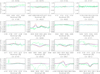 |
Fig. 11 As Fig. 10, but for HD 93128 (O3.5V), and a carbon abundance of [C/H] = 8.23 dex. |
| In the text | |
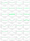 |
Fig. 12 As Fig. 9, but for HD 188209 (O9.5Iab), and a carbon abundance of 8.23 dex. |
| In the text | |
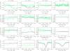 |
Fig. 13 As Fig. 10, but for HD 169582 (O6Ia), and carbon abundance of 8.53 dex. |
| In the text | |
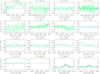 |
Fig. 14 As Fig. 10, but for CygOB2-7 (O3I), and a carbon abundance of 8.03 dex. |
| In the text | |
|
Fig. 15 Impact of X-ray radiation on the C IV 5801-12 lines, for a supergiant model with Teff = 40 kK (S40). Black: line profiles for the “standard” model without shocks; green: model with an intermediate X-ray strength; red: model with strong X-ray radiation. The dotted profiles refer to alternative, no-shock models with reduced carbon abundance, mimicking the effect of shock radiation. We note that the displayed sensitivity is strongest for the considered lines and parameter range, see text. |
| In the text | |
|
Fig. B.1 C II 5145, C III 5696, and C IV 5801 line profiles for model D30 (black lines, see Table 2) and similar models with relatively small changes in effective temperature (Teff) and gravity (log g). Upper panels: red lines correspond to a D30 model with Teff increased by 1000 K, the green lines to a model with Teff decreased by the same value, while the blue lines display the reaction to a decrease of Ṁ by a factor of three. Lower panels: red and green lines correspond to a D30 model with log g increased and decreased by 0.15 dex, respectively. |
| In the text | |
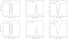 |
Fig. B.2 As Fig. 6, but for model D40, and C III 4068-70, instead of C II 5145. |
| In the text | |
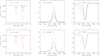 |
Fig. B.3 As Fig. B.1, but for model S30, and Δlog g = 0.1. |
| In the text | |
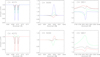 |
Fig. B.4 As Fig. B.2, but for model S40. |
| In the text | |
|
Fig. B.5 Carbon line profiles for model D35 (black), and dependence on stellar parameters, for our complete set of lines. The red and green solid line profiles correspond to an increase and decrease by 1500 K in Teff, respectively, whereas the red and green dashed profiles correspond to a variation of +0.2 dex and −0.2 dex in log g. |
| In the text | |
Current usage metrics show cumulative count of Article Views (full-text article views including HTML views, PDF and ePub downloads, according to the available data) and Abstracts Views on Vision4Press platform.
Data correspond to usage on the plateform after 2015. The current usage metrics is available 48-96 hours after online publication and is updated daily on week days.
Initial download of the metrics may take a while.