| Issue |
A&A
Volume 614, June 2018
|
|
|---|---|---|
| Article Number | A44 | |
| Number of page(s) | 19 | |
| Section | Extragalactic astronomy | |
| DOI | https://doi.org/10.1051/0004-6361/201732377 | |
| Published online | 12 June 2018 | |
Testing the accuracy of reflection-based supermassive black hole spin measurements in AGN
1
SISSA,
Via Bonomea 265,
34135
Trieste, Italy
e-mail: This email address is being protected from spambots. You need JavaScript enabled to view it.
2
INAF - Osservatorio Astrofisico di Arcetri,
Largo E. Fermi 5,
50125
Firenze, Italy
3
Dipartimento di Fisica e Astronomia, Università di Firenze,
Via G. Sansone 1,
50019
Sesto Fiorentino (Firenze), Italy
Received:
28
November
2017
Accepted:
19
February
2018
Abstract
Context. X-ray reflection is a very powerful method to assess the spin of supermassive black holes (SMBHs) in active galactic nuclei (AGN), yet this technique is not universally accepted. Indeed, complex reprocessing (absorption, scattering) of the intrinsic spectra along the line of sight can mimic the relativistic effects on which the spin measure is based.
Aims. In this work, we test the reliability of SMBH spin measurements that can currently be achieved through the simulations of high-quality XMM-Newton and NuSTAR spectra.
Methods. Each member of our group simulated ten spectra with multiple components that are typically seen in AGN, such as warm and (partial-covering) neutral absorbers, relativistic and distant reflection, and thermal emission. The resulting spectra were blindly analysed by the other two members.
Results. Out of the 60 fits, 42 turn out to be physically accurate when compared to the input model. The SMBH spin is retrieved with success in 31 cases, some of which (9) are even found among formally inaccurate fits (although with looser constraints). We show that, at the high signal-to-noise ratio assumed in our simulations, neither the complexity of the multi-layer, partial-covering absorber nor the input value of the spin are the major drivers of our results. The height of the X-ray source (in a lamp-post geometry) instead plays a crucial role in recovering the spin. In particular, a success rate of 16 out of 16 is found among the accurate fits for a dimensionless spin parameter larger than 0.8 and a lamp-post height lower than five gravitational radii.
Key words: methods: data analysis / techniques: spectroscopic / quasars: supermassive black holes / X-rays: galaxies
© ESO 2018
1 Introduction
An isolated astrophysical black hole is characterized by two fundamental quantities: its mass, M, and its angular momentum, J; this assumes charge neutrality, and thus the space-time is described by the Kerr metric (Kerr 1963). The mass can be considered as a scaling factor for distances, timescales and luminosities. In other terms, this means that accreting black holes with masses ranging from stellar mass, as seen in X-ray binaries, to supermassive black holes (SMBHs), as seen in active galactic nuclei (AGN), have a similar spectro-temporal behaviour once the luminosities and timescales are scaled properly (McHardy et al. 2006). However, the angular momentum (usually described in terms of the dimensionless spin parameter, a* = Jc∕GM2), which a black hole acquires from its growth history, is arguably the most interesting parameter as it affects the Kerr metrics leading to various properties of astrophysical importance. Theoretically, the spin values range in the [−0.998, 0.998] interval (Thorne 1974). These limits are found without considering magnetohydrodynamic (MHD) accretion. In fact, the magnetic fields of the plunging regions should give rise to torques that tend to reduce the maximum spin (~0.9−0.95) that can be achieved by a black hole (e.g. Gammie et al. 2004; McKinney & Gammie 2004).
Measurements of SMBH spins are a key ingredient for understanding the physical processes on scales ranging from the accretion disc out to the host galaxy. In fact, the spin determines the position of the innermost stable circular orbit (ISCO) of the accretion disc and of the event horizon, which are 1.24 and 1.06 rg for a maximally rotating black hole, and 6 and 2 rg for a non-spinning black hole, respectively, where rg = GM∕c2 is the gravitational radius. Hence, it has been shown that for a Schwarzschild black hole (a* = 0) half of the energy is radiated within ~30 rg, while half of the radiation emerges from within ~5 rg for a rapidly spinning black hole (e.g. Thorne 1974; Agol & Krolik 2000). This can be translated into an increase of the radiative accretion effeciency (η) from η = 0.057 for a* = 0, to 0.32 for a* = 0.998. Vasudevan et al. (2016) assumed a toy model with a bimodal spin distribution and showed that a SMBH population where only 15% of the sources are maximally rotating can produce 50% of the cosmic X-ray background (CXB) owing to their high radiative efficiency. Moreover, these authors showed that the spin bias is even larger in flux-limited surveys, since half ofthe CXB can be accounted for if only 7% of the sources have a spin of 0.998 (see also Brenneman et al. 2011).
The SMBH spin distribution is also fundamental for understanding the SMBH-host galaxy co-evolution. In fact, the angular momentum of a black hole matures over cosmic time and its final value is determined by the accretion and merger history of the galaxy. For instance, mergers tend to spin down the black hole (Volonteri et al. 2013), while the SMBH spins up through prograde accretion of material through the galactic disc (King et al. 2008). It has also been shown that highly energetic outflows in the form of relativistic winds (Gofford et al. 2015) or jets (e.g. Blandford & Znajek 1977; King et al. 2015) are affected by the accretion flow, hence their strengths are somehow related to the SMBH spin. These forms of mechanical AGN feedback, in addition to the high radiative efficiency, seem to play a crucial role in the evolution of the host galaxy and its star formation history. Hence, understanding the growth of SMBHs and their spin distribution is a key point for our understanding of the larger scale structure of the Universe (see Fabian 2012, for a review about AGN feedback).
In addition to the importance of SMBH spin in cosmology and galaxy evolution, the nuclear regions in AGN can be considered as unique laboratories to directly test the effects of general relativity, which manifest themselves as extreme physical phenomena such as light bending (e.g. Miniutti & Fabian 2004) and reverberation lags (e.g. Fabian et al. 2009; Emmanoulopoulos et al. 2011; Kara et al. 2016). This requires high-quality X-ray observations. In fact, AGN are strong X-ray emitters and it is widely accepted that the X-rays arise from the innermost regions of the accretion disc where the primary continuum is due to the Comptonization of ultraviolet (UV) disc photons by a hot (~ 109 K) transrelativistic medium, usually referred to as the X-ray corona (e.g. Shapiro et al. 1976; Haardt & Maraschi 1993; Petrucci et al. 2001a,b). As the measure of the spin is strongly dependent on the irradiation and subsequent emissivity of the disc, its success is tightly connected to the study of the X-ray corona itself, whose nature and properties are still largely unknown.
2 Spin measurement methods and their limitations
The increase in number and quality of AGN spectra, at various wavelengths, allowed astronomers to attempt a determination of the SMBH spin parameters with a relatively high confidence. A variety of observed features are considered as good indicators of the black hole spin, such as continuum shape (e.g. Done et al. 2013), broad iron Kα line (Fabian et al. 2000), and quasi-periodic oscillations (QPOs; e.g. Mohan & Mangalam 2014). Recently, the detection of gravitational waves through the coalescence of black hole pairs founded a new technique to constrain the spins of non-accreting black holes (Abbott et al. 2016a,b). There are several advantages and caveats relative to each method. Continuum fitting, for instance, can be applied to any AGN for which continuum emission is detected and has been applied to sources out to redshift ~ 1.5 (e.g. Capellupo et al. 2015, 2016). However, one of the main drawbacks of this method is that it requires a broad and simultaneous wavelength coverage, which usually exceeds the capabilities of a single observatory, in order to determine properly the shape of the relevant part of the spectral energy distribution (i.e. optical to X-rays). This method requires accurate estimates for the black hole mass, disc inclination, and distance, which are typically derived from optical data. Furthermore, the continuum fitting method can be applied effectively only when the peak of the emission from the accretion disc can be reasonably probed. Since most AGN spectra peak in the extreme UV, this range is only accessible by current detectors in high-redshift objects, at the expense of a rather modest quality for the corresponding X-ray spectra (e.g. Collinson et al. 2017). As for the QPOs, they are common in Galactic binaries while few examples exist in AGN light curves, most of which are statistically marginal and/or controversial (apart from the notable case of RE J1034+396; Gierliński et al. 2008). Their detection requires long monitoring, high signal-to-noise ratio (S/N), and a proper modelling of the continuum power spectrum (Vaughan & Uttley 2005, 2006).
The most direct and robust measurements to date are those obtained through the detection of a strong relativistic reflection feature in the X-ray spectra. This method can be applied to a wider black hole (BH) mass range. X-ray spectra of AGN can be expressed as a sum of several components, in particular a primary continuum that is well approximated by a power law with a high-energy exponential cut-off and ionized and/or neutral reflection that is detected in most of the sources, arising either from the accretion disc within a few gravitational radii from the BH or from distant Compton-thick material (the broad line region or the molecular torus), respectively (e.g. Lightman & White 1988; George & Fabian 1991; Ghisellini et al. 1994; Bianchi et al. 2009). The resulting reflection spectrum is characterized mainly by the iron Kα emission line at ~6.4−7.0 keV and a broad component peaked at around 20–30 keV, known as the Compton hump. Special and general relativistic effects result in blurring the ionized reflection spectrum and asymmetrically broadening the Fe Kα emission line owing to the gravitational redshift and the motion of the emitting particles in the disc (see Fabian et al. 2000; Reynolds & Nowak 2003, for reviews). This method consists in fitting the X-ray spectrum of a given source with a reflection model accounting for the relativistic distortions that affect these features on their way to the observer. We mention some of the models that predict the relativistic line profile for a narrow line emitted in the rest frame of the accretion disc: diskline, laor, kyrline, kerrdisk, relline as published in Fabian et al. (1989), Laor (1991), Dovčiak et al. (2004), Brenneman & Reynolds (2006), Dauser et al. (2010), respectively. The resulting shape of the reflection spectrum strongly depends on the parameters of the system. Hence, this method can be used not only to determine black hole spins but also to probe the innermost regions of the accretion discs, providing information about its inclination, ionization state, elemental abundance, and emissivity (see Reynolds 2014, for a review). However, there are known difficulties in determining the spins via X-ray reflection, which are mainly due to the complexity of (and some subjectivity in) modelling the AGN spectra, considering the various emission and absorption components that are known to be present, hence requiring high-quality data (e.g. Guainazzi et al. 2006; Mantovani et al. 2016).
An alternative absorption-based interpretation has been proposed to explain the apparent, broad red wing of the Fe line and the spectral curvature below 10 keV (e.g. Miller et al. 2008, 2009). According to this scenario, partial-covering absorbers in the line of sight (having column densities in the 1022−24 cm−2 range) plus distant (i.e. non-relativistic) low-ionization reflection, can produce an apparent broadening of the Fe Kα line similar to that caused by relativistic effects. Variability in the covering fraction of these absorbers would also provide a complete description of the observed spectral variability.
Contrary to stellar-mass BHs, whose spectra are much brighter and typically less complex, both blurred reflection and partial covering are relevant to the X-ray spectra of AGN. In fact, while the former process is able, in principle, to explain the spectral and timing properties of any accreting system, the rapid Compton-thin to Compton-thick (and vice versa) transitions seen in changing-look AGN (after Matt et al. 2003) imply that also partial covering must be taken into account. In a single-epochAGN spectrum, the effects of disc reflection and partial covering are often hard to separate or distinguish from each other, thus leading to a long-standing debate. However, thanks to the high-quality spectra provided by XMM-Newton (Jansen et al. 2001) and NuSTAR (Harrison et al. 2013) observations, which jointly cover a wide energy range from 0.3 keV up to 80 keV, it has now become possible to disentangle the two scenarios, as shown in the case of NGC1365 (Risaliti et al. 2013). Three different variable absorbers with column densities in the range 5 × 10²² − 6.5 × 1024 cm−2 and variable covering factors would be needed to explain the spectrum of the source below 10 keV. However, this absorption-only model fails to explain the hard X-ray spectrum in the 10–80 keV band, where the inclusion of relativistic reflection provides a statistically better description of the data (Risaliti et al. 2013; Walton et al. 2014). Furthermore, the latter model is also preferred on physical grounds, as the inferred bolometric luminosity in absorption-only scenarios is significantly higher compared to other indicators such as the [O III] λ5007 line. The case of NGC 1365 lends weight to the idea that X-ray reflection is indeed an effective means of measuring the spin of SMBHs, even when absorption is present.
3 Motivation and methods
Our main aim is to test the reliability of spin measurements when the spectra include additional components with respect to the simple primary continuum plus disc reflection configuration (i.e. always, in principle). In fact, the innermost emission components are generally subject to absorption by gas with column densities from NH < 1021 cm−2 to NH > 1024 cm−2 and ionization states from neutral to almost completely ionized. As demonstrated by the case of NGC 1365, the presence of a given absorption component can be better identified thanks to its variability. NGC 1365 is one of the unique sources showing frequent changes in its obscuration state. Recently, Risaliti (2016) summarized the various observational aspects of this source and proposed a multi-layer structure of the circumnuclear medium to explain all the observed absorption states and their variability. NGC 1365 has been observed several times in reflection-dominated states, suggesting the presence of a layer of neutral Compton-thick (NH > 1024 cm−2) absorber located at a distance of the order of or larger than that of the broad line region (Risaliti et al. 2007). The source is usually caught in a Compton-thin state, NH ~ 1023 cm−2, but the column can even occasionally drop down to NH ~ 1022 cm−2 (Braito et al. 2014). Furthermore, absorption lines have been detected when the source is not heavily obscured, indicating a stratification of absorbers with ionization states ranging from highly ionized (log ξ > 3)1 to mildly ionized (logξ ~ 1−2) down to neutral (logξ < 1). All these components and absorption states can be present in all AGN. However, their detection in a single source, even if at different times, is highly dependent, on the one hand, on our line of sight, and, on the other hand, on the chance to observe any given component when variability is present.
The repetition of measurements (via X-ray reflection) can result in inconsistent values of the spin parameter for a given source. The discrepancy is mainly due to the use of different components in modelling the spectra, such as the use of dual reflectors, partial-covering, and/or warm absorbers. For example, Patrick et al. (2011) analysed the Suzaku spectra of NGC 3783, among others, and found the spin parameter in this source is a* < −0.04. This result contradicts the high spin parameter (a*≥ 0.88) found by Brenneman et al. (2011) and Reynolds et al. (2012), who analysed the same observations.
The work presented in this paper is a preliminary study aiming to test, through the simulation of high-quality XMM-Newton and NuSTAR spectra (in the 0.3–79 keV range), the reliability of reflection-based SMBH spin measurements that can currently be achieved. A similar approach has been adopted recently by Bonson & Gallo (2016) and Choudhury et al. (2017), who simulated AGN spectra by assuming only two components: primary emission and relativistic reflection. Instead, we assume a more complex spectral configuration, closer to the real general case. This is presented below, along with a detailed description of how we simulated and fitted the data. We note that both of the aforementioned studies neglected the soft X-ray band, in which the soft excess can be a crucial driver of reflection-based spin determinations (e.g. Walton et al. 2013).
3.1 Simulation set-up
As mentioned above, various emission/absorption components can be present in the X-ray spectrum of any AGN. However, depending on the state in which the source is caught, we may be able to observe all or only some of these components. Generally, the Ockham’s razor argument is (or should be) applied during the spectral fitting, thereby avoiding the inclusion of unnecessary components. While this is the correct practice, we might miss a component that is actually present in the case of a single-epoch observation, either if the spectra do not cover a broad band or do not have enough S/N. We know from the literature the expected ranges of the parameters for the various components that are observed and are potentially present in any AGN spectrum. Hence, we can simulate the most general spectrum and then examine how well the model parameters are recovered using the common fitting techniques.
We simulated AGN spectra in the 0.3–79 keV band via the XSPEC v12.9.0s (Arnaud 1996) command FAKEIT and the XMM-Newton EPIC-pn (Strüder et al. 2001) and the NuSTAR response matrices in the 0.3–10 keV (with an exposure time of 90 ks)2 and 3–79 keV (with an exposure time of 100 ks, i.e. 50 ks per focal plane module) ranges, respectively. The spectra were binned not to oversample the FWHM resolution by a factor larger than 3 and 2.5 for XMM-Newton and NuSTAR, respectively. Then, we grouped the spectra, for both instruments, to ensure a minimum S/N of 5 in each energy channel. The simulations are intended to represent single-epoch observations of bright low-redshift AGN, similar to the observed sources, using XMM-Newton and NuSTAR simultaneously. Hence, we defined a generic parent model that contains the various expected emission and absorption components. The former are described below through their Xspec spectral counterparts:
-
APEC: thermal diffuse emission at soft X-rays arising from the host galaxy in the cases when the star formation rate is enhanced and/or from gas photoionized by the AGN in the narrow line region (see Nardini et al. 2015, for the reference case of NGC 1365, and references therein for other notable sources). The parameters of this model that were varied during the simulations are the temperature of the gas (kT) and its abundance in solar units (from Grevesse & Sauval 1998).
-
RELXILLLPv0.4a: primary emission plus blurred relativistic reflection from ionized material, assuming a lamp-post geometry for the emitting source (Dauser et al. 2013; García et al. 2014). The free parameters of this model are the photon index (Γ) of the incident continuum, the height of the lamp post (h, in units of rg), the spin parameter (a*), and the inclination (i), ionization (ξd), and iron abundance (AFe in solar units) of the accretion disc. We kept the high-energy cut-off fixed to 300 keV. The reflection fraction is computed self-consistently within the model and fixed to the lamp-post value (fixReflFrac = 1), as defined in Dauser et al. (2016). This also implies that the disc emissivity as a function of radius is fully determined by the height of the X-ray source.
-
XILLVER: neutral reflection arising from distant material by fixing the ionization parameter, inclination angle and iron abundance of the reflector to logξ = 0, i = 45° and AFe = 1, respectively. For simplicity, we tied the values of the photon index and the high-energy cut-off of this component to those of the primary continuum.
As for the absorption components, we modelled the Galactic column using the PHABS model and assuming NH = 5 × 1020 cm−2. We assumed that the intrinsic absorption can affect only the innermost emission components (primary continuum and relativistic reflection), and we considered the following configuration:
-
WARMABS: fully covering warm absorption modelled through an XSTAR table (Kallman & Bautista 2001) having an input continuum with a photon index of 2. Although it is usually seen in outflow (e.g. Braito et al. 2014, and references therein), we assume for simplicity that this component is at rest in the local frame. The free parameters of this model are the column density NH, wa and the ionization parameter of the absorber ξwa.
-
ZPCFABS: two layers of partially covering neutral absorbers that can represent the various neutral-absorption states (from Compton-thin to Compton-thick regimes). We let free to vary the column densities NH, 1∕2 and the covering fractions CF1∕2 of both absorbers.
The final model can be written in XSPEC terminology, neglecting Galactic absorption, as follows:

A scheme of the proposed configuration is shown in Fig. 1. We report in Table 1 the input range chosen for each of the free parameters considered in the simulations. The redshift of the simulated source is fixed at 0.02. We kept the normalizations of the various emission components free, and the only limitation is that the observed flux is between 1 and 3 mCrab in the 0.3–10 keV range (resulting in ~ 3 × 10⁵−106 counts, for the XMM-Newton spectra).
We note that the configuration we adopted may have some caveats on physical grounds. For instance, we neglected Compton scattering out of and into the line of sight for partial coverers with column densities NH > 1024 cm−2. In fact, this would make the structure of the model much more complicated. On the one hand, accounting for the scattering into the line of sight would require arbitrary geometrical assumptions. On the other hand, the combinationof partial covering and scattering out of the line of sight is not trivial in terms of model definition and handling. Even if these effects were treated properly, the actual physics of a real system would still be likely much more complex than the model we adopted. For example, the distant reflection is assumed to arise from a plane-parallel slab with an intermediate inclination of 45°, but this is just a coarse representation of the expected geometry of the reflector (see e.g. Yaqoob 2012). Moreover, this component might not be completely neutral; its ionization is low but not negligible, which leads to some heating near to the surface of the reflector (García et al. 2013). This mainly shifts the narrow iron K feature to higher energy. An additional complexity could be also due to the possible presence of multi-temperature thermal emission, a more complex structure of the warm absorption, or other forms of scattering into the line of sight. Finally, it should be kept in mind that the actual geometry of the X-ray corona is largely unknown. The point-like, lamp-post corona is a convenient approximation, but it also has some clear physical limitations, for instance a compactness problem similar to gamma-ray bursts (e.g. Fabian et al. 2015; Dovčiak & Done 2016). It is worth stressing, however, that none of our assumptions affect our results as long as the simulations and spectral fitting are performed in a self-consistent way.
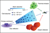 |
Fig. 1 Schematic (not to scale) of the proposed configuration, presenting the various emission and absorption features that we consider in this work (see Sect. 3.1 for details). |
Key parameters used to perform the simulations with the corresponding input range, for the various emission and absorption components.
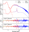 |
Fig. 2 Toppanel: example of the simulated XMM-Newton (red) and NuSTAR (blue) spectra (corresponding to simulation G8) together with the various components of the theoretical model assumed. The primary emission plus ionized reflection (dashed lines), neutral reflection (dash-dotted lines), and thermal emission (dotted lines) are shown. Middle and bottom panels: the χ2 residuals obtained by the two separate fits are indicated (see Sect. 3.2 for details). |
3.2 Fitting procedure
In order to reduce the observer-expectancy effect, each simulation was created by one member of the group and fitted blindly by the two other members separately. The various spectral components mentioned above were allowed to be present or absent in any simulation (and fit), except for the primary continuum plus ionized reflection component, which was always included by construction. We first simulated a general set of 15 simulations (5 simulations per person; hereafter SetG, we refer to these simulations as G1–G15). The simulated parameters were allowed to vary within the input range, whilein the fits they were free to vary without any restriction, apart from neglecting negative spins and heights below 2 rg. The Ockham’s razor criterion was followed in the spectral analysis. A fit was considered as satisfactory at personal discretion, provided that 1) the overall statitistics was good, 2) the χ2 value represented a stable minimum, and 3) no obvious residuals were present. This does not ensure that the accepted fit is strictly the best possible. Indeed, in some cases only a local χ2 minimum is found, revealing how critical this kind of analysis can be in practice (see Sect. 5 for a more detailed discussion).
An example of the simulated data with the theoretical model and the corresponding residuals from the two different fitsis shown Fig. 2. Errors on the parameters are calculated from Markov chain Monte Carlo (MCMC)3, using the Goodman-Weare algorithm (Goodman & Weare 2010) with a chain of 510 000 elements (170 walkers and 3000 iterations), and discarding the first 51 000 elements as part of the “burn-in” period. We show in Fig. 3 the results of the MCMC analysis for the best-fit reflection parameters found for the simulated spectrum presented in Fig. 2.
4 Results
We present in Table 2 a qualitative summary of the results we obtained from the blind spectral analysis, based on the classification criteria defined below. While these criteria are to a certain extent (but unavoidably) arbitrary, none of the conclusions of the paper are substantially modified.
Individual parameters. For all the parameters, except for the spin and, to a lesser extent, iron abundance, the measurements are generally very well constrained. Thus, we define both a full and a fair success criterion. The former (denoted by the ✓ sign) is met when a measurement is consistent with the input value within a confidence level of 90%, while the latter (denoted by the ★ sign) is met when the fitted and input values are formally inconsistent, but agree with each other within a 10% uncertainty4. All the other cases are classified as failures (denoted by the ✗ sign).
Spin classification. Since the measure of the spin is the main aim of our study and the spin is the parameter that shows the most complex behaviour in the fits, we adopted a different approach to classify the goodness of our constraints on the spin parameter. We divided the 0–0.998 spin range into three bands: low spin (a* ∈ [0, 0.4[), intermediate spin (a*∈ [0.4, 0.8[), and high spin (a*∈ [0.8, 0.998]). Hence, we classified the measurements based on the following criteria: (a) full success if the measured value is consistent with the input one within the 90% confidence level and the uncertainty range is within a single spin band; (b) fair success if either the measured value is consistent with the input value within the 90% confidence level but the uncertainty range covers two spin bands, or the measured value is not consistent with the input value but the uncertainty range is within the same single band that contains the input value; (c) undetermined (denoted by the ? sign) if the measured value is consistent with the input one but the uncertainty range covers three spin bands; and (d) failure for the other cases.
Fit accuracy. Irrespective of the values of the individual parameters and their degree of adherence to the input values, we also defined the following quality criteria for the accuracy of the whole fit: a) excellent if the adopted model is correct and the fit statistic is within a Δ χ2 of 2.3 from the putative absolute minimum (see below); b) good if either the model is correct and the distance from the absolute minimum is Δ χ2 < 9.2, or the model misses a component that turns out to be significant at less than 99%; c) inaccurate in all the other cases, including overfitting. The absolute minimum is evaluated as  , where
  is obtained by applying a posteriori the input model and
  are the results from the blind spectral analysis (provided that the correct model is used). We found that 18 out of 30 fits were excellent, 4 out of 30 were good, and 8 out of 30 were inaccurate. We note that the application of the correct model (i.e. corresponding to the input one), as becomes evident below, does not imply that the input parameters are individually recovered with success (see Fig. 3). We stress again, however, that even inaccurate fits are fully acceptable on statistical grounds and meet the three conditions listed in Sect. 3.2.
We summarize below the constraints that we obtained on the relevant parameters that are always present in the model by construction, distinguishing between accurate (either good or excellent) and inaccurate fits as follows:
-
The measure of the spin parameter was a full/fair success in 7 + 4 cases, while it was undetermined/failed in 5 + 6 cases out of the 22 accurate fits. In the 8 inaccurate fits, 6 spins were fairly retrieved and 2 were undetermined. Low and intermediate spins (i.e. lower than 0.8) were present in 9 out of 15 simulations (i.e. 18 spectral fits, 13 of which were accurate). A low spin value was determined correctly and well constrained in only 1 out of 18 cases. The measure of the spin was fairly successful in 5 cases and it was undetermined in 6. However, for the 6 high-spin simulations (9/12 accurate fits), the measurements were successful in 10 cases (5 fully, 5 fairly), undetermined once, and the only failure was in a fit classified as excellent. In summary, the two different fits corresponding to the same simulated spectrum might result in different best-fit values of the spin parameter if one of the fits hits a secondary minimum or makes use of a wrong model, thus classified as inaccurate. However, even fully successful fits are not always able to recover the correct value of the spin, with a clear preference for high values.
-
The height of the lamp post, which is the other key parameter that determines the strength of the reflection component in the observedspectra, was measured with success in 7 (full) plus 2 (fair) cases, while it failed in the remaining 13 of the 22 accurate fits. However, 3 more full successes were found among the 8 other fits. The role of the source height is further discussed later on.
-
The disc inclination was measured with success in 16 plus 4 of the accurate fits (2 failures) and 2 plus 2 of the inaccurate fits (4 failures).
-
The photon index was measured successfully in all cases, of which 20/30 were a full success. We found a maximum difference between the measured and input photon index of ΔΓ = 0.12.
-
The discionization parameter was retrieved with success in 13 plus 2 of the accurate fits (with 7 failures) and 3 of the inaccurate fits (5 failures).
-
The measure of iron abundance was fully successful in 15/22 accurate fits and in 4/8 inaccurate fits, and unsuccessful in all the other cases.
As already noted, the failure in measuring the single parameters might also occur in cases in which the fit is highly accurate for both analysts (e.g. G8, G11), which is a possible indication of complex degeneracies.
The various simulated spectra for Set G together with their corresponding residuals are presented in Fig. A.1. The best-fit results relative to the reflection components are presented in Fig. 4, while those for the absorption and thermal components are presented in Fig. 5. Table A.1shows the input and best-fit values of the lamp-post height and spin parameters. We report the best-fit χ2 ∕d.o.f. values in the same table.
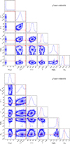 |
Fig. 3 Results of the MCMC analysis for the relevant best-fit reflection parameters corresponding to the two different spectral fits shown in the middle and bottom panels of Fig. 2. The red lines correspond to the input values assumed in order to create the simulations. We show the χ2 values obtained from the corresponding best fit, whose accuracy as a whole is excellent in both cases. The individual parameters, however, are not all correctly retrieved. |
5 Discussion
We simulated in this work high-quality single-epoch spectra of AGN at low redshift in the 0.3–79 keV band using the responses of both XMM-Newton and NuSTAR. We assumed a general spectrum that includes, in addition to the primary emission, both ionized and neutral reflection, thermal emission, a warm absorber, and two layers of neutral partially covering absorbers. While in most cases the blind fitting procedure should be considered as successful, this fails in retrieving all of the individual input parameters. Below we examine the possible causes.
5.1 The Kerr BH case
As noted in Sect. 4, spectral analysis tends to recover high input spins better than low/intermediate spins: 10 out of 12 high-spin measurements were at least fairly successful, while only 7 out of 18 low/intermediate spins were reasonably retrieved. Furthermore, the measured spin distribution, as reported in the literature, shows a clear tendency towards high spins (e.g. Walton et al. 2013; Reynolds 2014; Vasudevan et al. 2016). This evidence was the main motivation for us to simulate a set of high-spin spectra (hereafter Set K). Thus, we generated a set of 9 simulations (3 simulations per person) by fixing the spin parameter to its maximum allowed value; we refer to these simulations as K1–K9. However, the spin parameter was free to vary within the 0–0.998 range during the spectral fitting. The constraints on the best-fit parameters of the reflection and absorption components are presented in Table 2, and plotted together with the corresponding input values in Figs. 5 and 6, respectively. The spin was retrieved successfully in 6 (3 fully and 3 fairly) of the 11 accurate fits, with 5 failures, while the 7 inaccurate fits returned 2 fairly constrained spins (with 5 failures). In total, only 18 out of 30 high-spin cases (in Sets G and K) were a success: 13 (8 plus 5) are obtained in the 20 accurate fits, while other 5 fair successes still emerge from the 10 inaccurate fits. This suggests that, even though it plays an important role, the spin is not the only factor that may lead to a positive result in recovering its input value.
5.2 Effects of absorption
We summarize below the constraints we obtained on the absorption components in Sets G and K. We note that these components can be added/removed arbitrarily. 1) The fully covering warm absorber is included in 23 simulations (equivalent to 46 fits). Its column density and ionization parameter were positively recovered in 34 (30 full plus 4 fair successes) and 38 (36 plus 2) cases, respectively. Both rates are higher than the incidence of accurate fits (32/46). 2) The partial-covering low-column absorber is present in 21 simulations. Its column density and covering fraction were measured successfully in 25 plus 1 and in 28 plus 1 cases, respectively, against 25 out of 38 accurate fits (in 4 cases this component is missed in the spectral analysis). 3) The partial-covering high-column absorber is present in 19 simulations. Its column density and covering fraction were measured successfully in 23 plus 12 and 24 plus 12 cases, respectively, when the accurate fits are 24 out of 37 (this component is missed only once).
Summarizing, the properties of the absorbers are correctly estimated in the majority of the blind fits. Even though the number of simulations that we performed is statistically small, we can still derive a general idea of the degeneracy that may be present between the reflection-based models and the complex absorption model. It may happen that the inclusion of an absorber that is not present intrinsically mimics some of the relativistic effects on the spectrum, thus resulting in a wrong measurement of the spin parameter. However, it seems that absorption plays only a marginal role in the ability of measuring spins, as the overall absorption configuration in the fits was correct in 37 out of 48 cases. These issues are further investigated in Sects. 5.5 and 5.6.
Summary of the success/failure in measuring the relevant parameters for the three simulation sets.
5.3 The bare sources case
In order to completely remove the uncertainties associated with absorption effects, we performed an additional set of 6 simulations (two per person) of bare sources, without including any intrinsic absorption (hereafter Set B, we refer to these simulations as B1–B6). The input model of this set can be written in XSPEC terminology, neglecting Galactic absorption, as follows: model = RELXILLLP + XILLVER + APEC. The simulated spectra and the χ2 residuals are presented in Fig. A.1. The input parameters together with the best-fit values are plotted in Fig. 6. We summarize in Table 2 the qualitative constraints on the parameters that we obtained for this set. Four of these simulations involved a high spin value, and two cases each correspond to a lamp-post height ≤ or > 5 rg. All the successful spin measures (1 full and 3 fair, with 3 out of 4 accurate fits) occurred for a low height of the source. Interestingly, at low height even a smallspin is correctly retrieved (1 full and 1 fair success in 2 out of 2 accurate fits). Conversely, when the height of the lamp post is larger than 5 rg, the measureof the spin always fails, irrespective of its value and despite the good rate (4/6) of accurate fits. The other disc reflection parameters were all well constrained in all cases, except for the Fe abundance in a single instance. Asfor the thermal and distant reflection components, they were both correctly assessed in 10 out of 12 fits.
In total, 19 out of the 30 simulations (i.e. 38 out of 60 fits) were performed asssuming maximally rotating black holes. The spectral analysis resulted in 22 successes in the measure of the spin (9 full and 13 fair), with 1 undetermined and 15 failed cases, for 25/38 accurate fits. Remarkably, when we consider only the simulations performed with a low lamp-post height, the total count features all the 22 successes and only 2 failures, for the same fraction (16/24) of accurate fits. This strongly suggests that the height of the primary X-ray source is the most critical ingredient for an accurate measure of black hole spin.
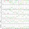 |
Fig. 4 Input values (black dots) of the reflection parameters assumed for creating the various simulations (for Set G). The best-fit values obtained for the various parameters are shown as squares and diamonds for the two different realizations. The colour code refers to the quality of the fit as a whole: green for excellent, yellow for good, and red for inaccurate (see text for details). The error bars represent the 90% confidence levels obtained from the MCMC analysis. |
5.4 Effects of the lamp-post height
In the light of these findings, we further explored the dependence of our results on the input lamp-post height. Half of the simulations were perfomed assuming an input lamp-post height lower or equal to 5 rg. In general, these heights were measured successfully in 21 (16 plus 5) fits, with 5 full successes coming from the 9/30 inaccurate fits. Three of these 15 simulations were performed assuming a low input spin parameter. The fit was accurate in 5 out of 6 cases, returning 2 successes in the measure of the height and 4 (1 plus 3) in that of the spin.
By considering the second half of the simulations, with a lamp-post height larger than 5 rg, we find that the height was correctly estimated in 6/30 fits only despite the 21 out of 30 accurate fits. In 5 out of 30 spectral fits we were able to recover the spin (2 full and 3 fair successes), while in 6 out of 30 cases the spin was undetermined. Eight of these 15 simulations were performed assuming a low spin. As already noted, the high spin and large height case gave 1 undetermined and 13 failures, despite the 9 out of 14 accurate fits. This apparently suggests that, at large heights, the value of the spin has little weight, and the chance of success in its measure is not only small but also random (i.e. depending on several other factors such as iron abundance). In this sense, the preference for low spins is most likely a bias, so any measure at large heights should be taken with caution (see also Fabian et al. 2014).
The full summary is given in Table 3.
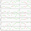 |
Fig. 5 Similar to Fig. 4 but for the absorption parameters (top panels) and the gas temperature of thermal emission component (last panel), presenting the results for sets G and K. The column densities are in units of 1022 cm −2. |
5.5 Model dependence
By construction, the disc reflection component is always included in both the simulated models and the fitted models, while the presence of all the other components, either additive (distant reflection, thermal emission) or multiplicative (warm, cold absorption) is arbitrary. This allows us also to investigate the impact of model dependence on the ability to accurately recover the reflection parameters. Considering all the simulations from Sets G, K, and B, soft X-ray thermal emission was present in 27 out of 30 cases, and was missed in only one out of the 54 relevant fits (K4a). Of the 3 out of 30 cases where it was not required, it was included in 5 out of 6 fits (G4a, b, G7b, B1a, b). Correctly accounting for this component or not seems to have little effect on the spin determination. Interestingly, its inclusion does not necessarily undermine the measure of the spin, but the accuracy is lower (compare the results of G7b versus G7a; Table 2. We note that model G7 isa low-spin, moderate-height case). In total, this component was measured successfully in 50 out of 53 spectral fits.
While the soft thermal component is easier to distinguish from the smooth, blurred reflection, the contribution from the distant reflector can significantly modify the shape of the Compton hump above 10 keV. This is present in 29 out of 30 models. It is missed once, and added instead in both fits of the single model (K5) where it was not originally included. This is a maximum-spin, low-height case, which, as we have seen, should have a higher chance of success. Indeed, both fits meet the fair success criterion for the spin. However, we could argue that the inclusion of distant reflection prevents us from obtaining more stringent constraints. In total, the normalization of this component was measured succesfully in 51 out of 57 spectral fits.
Absorption is allowed in 24 models only (G and K Sets). The fully covering, warm layer is present in 23 out of 24 simulations. Remarkably, it is never missed and never added. This suggests that the features imprinted on the spectrum from mildly (or even highly) ionized gas in the line of sight are relatively easy to identify, at least at the X-ray brightness level of the simulated spectra. Hence, we expect this component to have no significant effect on the measure of the spin. In reality, however, the different treatment of warm absorption might lead to incompatible spin measures for the same data set of the same source, as in NGC 3783 (Brenneman et al. 2011 versus Patrick et al. 2011). The micro-calorimeters on board Athena and, possibly, earlier X-ray missions such as Arcus (Smith et al. 2016) and XARM will conclusively remove this source of ambiguity.
The lower column partial-covering absorber is included in 21 out of 24 models, while the higher column partial-covering absorber in 19 out of 24. The former is missed 4 times and added in 2 out of 6 fits, the latter is missed once and added in 4 out of 10 fits. Without distinguishing between the relative column densities, the configuration of the partial-covering, cold absorber consists of a single layer in 6 out of 24 cases and of a double layer in 17 out of 24 cases. No cold layers are included in the remaining case (G5), but they are both used in G5b, leading to an undetermined spin measure (as opposed to a fair success for G5a, where the correct model is applied). Two layers instead of the single one required are adopted in 5 out of 12 fits, while one of the two layers is missed in 5 out of 34 fits. Surprisingly, the addition of a layer does not always preclude a decent (or even good) measure of the spin (e.g. G2b), although the statistical significance of the second layer in these cases is most likely marginal. Conversely, all the 5 cases in which a layer is missed correspond to failures or indetermination in the spin measurement. We conclude that the effects of partial covering and of relativistic reflection, when high-quality broadband spectra are available, can be generally well distinguished from each other. We further discuss this point in the next section.
Summary of the constraints on determining the spin showing its dependence on the lamp-post height.
5.6 Reflection versus partial covering absorption
According to some interpretations (e.g. Miller et al. 2008), no relativistic signature is needed to explain the spectra (and variability) of most AGN. This is a natural consequence of the substantial statistical equivalence between absorption- and reflection-based models, especially when the spectra are complex and require some combination of both ingredients. The relative dispute was initially concentrated on the nature of the Fe K line broadening since the partial covering absorption could reproduce both the smooth, extended red wing of the putative relativistic line as a gentle continuum curvature and its blue horn as an absorption edge. The appearance of tentative hard X-ray excesses in the Suzaku era added a further controversial element, which could be explained either as a Compton reflection hump (e.g. Walton et al. 2013) or as a signature of Compton-thick absorption (e.g. Tatum et al. 2013), thus reinforcing the polarity between the two mainstream scenarios. The advent of NuSTAR, providing high-quality spectra also above 10 keV, accurate background subtraction, and substantial overlap with the band covered by the other X-ray observatories, can greatly reduce this persistent ambiguity.
While, in principle, the ambiguity works in both ways, in our simulations we did not assume any pure partial-covering configuration (i.e. with no disc reflection), so we cannot verify whether an absorption layer could be missed by overestimating the amount of reflection. This is not the scope of our work. In fact, in this context it is more interesting to explore the possibility for the simulated models to be adequately reproduced without considering any relativistic component. We therefore checked the consequences of replacing the relxilllp component in our fits with a simple power law, in which the cut-off is fixed at 300 keV for consistency with the primary continuum in the parent model. This is equivalent to fixing the reflection fraction in relxilllp to zero. In order to compensate for the lack of disc reflection, we allow for a larger complexity in the absorption configuration. It turns out that only 1 of the 30 simulated spectra could be perfectly described also by a pure partial-covering model, as the relative fits would meet all of our acceptance criteria, namely good statistics and lack of residuals. This is G10 (χ2 ∕d.o.f. = 397∕394), where three cold layers are required: NH, 1 = 6 × 1021 cm−2 (CF1 = 1), NH, 2 = 5.5 × 1023 cm−2 (CF2 ~ 0.1), and NH, 3 = 3.6 × 1024 cm−2 (CF3 ~ 0.25). The fully covering, thinner layer is perfectly matched to a component of the input model, whose second layer has NH= 1.9 × 1024 cm−2 and CF = 0.26. Although G10 is a low-spin (a* = 0.12), large-height (h = 32 rg) case, a much more complex (and rather extreme) absorption pattern is required to compensate for the lack of disc reflection in the fit.
In three other cases (G14, K4, and K9) the reduced χ2 is fair (1.02, 1.10, and 1.04, respectively), and two layers have similar (even if not strictly consistent) properties to the input components. There are, however, some clear residual structures that make the absorption-only models not satisfactory. A third partial-covering layer is not statistically required. At low S/N, these spectra (with maximal spin but h > 5 rg) could be easily misinterpreted. A peculiar case is that of G5, where no cold absorbers are included in the simulation. This spectrum can be well fitted by a power-law continuum (χ2∕d.o.f. = 479∕477) that is subject to warm absorption only with the exact input parameters. Even if the disc reflection component in this case is very smooth and featureless, a model where this is correctly accounted for (G5a; χ2 ∕d.o.f. = 449∕473) is still statistically preferred (at the >4σ level based on the corrected Akaike Information Criterion usually adopted for non-nested models; Akaike 1974). It is likely that the contribution from disc reflection would be missed in lower quality data. A handful (≤ 5) of other cases, in principle, could become acceptable after the inclusion of a third partial-covering layer if the spectra were fainter by at least an order of magnitude with respect to the simulated spectra, which could mask the residuals within the photon noise. We note, however, that such a complex absorption configuration (even if real) should be rejected as a form of data overfitting at low S/N. We conclude that in most cases (26 out of 30), including all the Set B of bare spectra, disc reflection cannot be missed or mimicked by absorption effects in high-quality broadband X-ray spectra. The problems with its identification arise when the reflected spectrum is extremely smooth, so this could become a non-negligible issue if the X-ray corona is radially extended and thus responsible for the Comptonization of the relativistic signatures from the inner disc (see Steiner et al. 2017).
An interesting outcome of our analysis is that the failed spin measurements have a nearly flat distribution, which is clearly different from those reported in the literature. We plot in Fig. 7 the distribution of spin measurements listed in Vasudevan et al. (2016) together with that of wrong and undetermined measurements from our blind spectral analysis. As the uncertainties on the individual entries are rather large for both samples, we do not attempt any statistical test to compare quantitatively the two distributions. We note, however, that, while the selection effects leading to an observed spin distribution peaked towards higher values are well known (e.g. Brenneman et al. 2011), our results seem to discard any systematics or biases associated with possible reflection versus absorption spectral degeneracies.
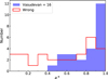 |
Fig. 7 Distribution of spin measurements from Vasudevan et al. (2016) (blue histograms) and the distribution of wrong and undetermined measurements (red histograms) obtained from the simulations performed in the current work. |
5.7 Simulations with Athena
To verify whether the failures require an even larger data quality (hence inaccessible to the current X-ray observatories), we chose two models for which the measured values of the spin were either undetermined (G6) or wrong (G11) despite the excellent accuracy of both fits. Based on our results, both cases are expected to be rather challenging, as they involve intermediate black-hole spin and large lamp-post height. We then simulated the same input model using the response files (with an exposure time of 100 ks) of the Wide Field Imager (WFI; Rau et al. 2013), one of the two scientific instruments proposed for the Athena X-ray observatory (Nandra et al. 2013). We performed an MCMC analysis as described in Sect. 3.2. For model G6, which has h = 17 rg, the results are similar to those obtained by the spectral analysis of the joint XMM-Newton and NuSTAR spectra. Even with WFI, the measured value of the spin remains undetermined, as shown by the a* −vs − h contour plots in Fig. 8. For model G11, which has almost the same input spin but lower height (8 rg), the measured spin remains inconsistent with the actual value of 0.7, but it is now much closer to this value (~ 0.9 against 0.2).This test, although unsuccessful, confirms the main indication of our study, i.e. the importance of a small lamp-post height (hence an effective illumination of the innermost disc) for an accurate measure of the BH spin. However, one of the limitations of fitting the spectra with Athena is the incapability of probing the Compton hump at high energies. We will further investigate this issue in a future work, where we will also consider the potential of high-resolution spectroscopy.
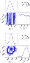 |
Fig. 8 Black hole spin vs. lamp-post height contour plots obtained by the MCMC analysis obtained from the best-spectral fits of G6 (top panel) and G11 (bottom panel), performed using the Athena-WFI response files. The input spin and height values (red lines) are listed on the top right corner of each panel for the corresponding simulation. |
6 Conclusions and future work
The measure of black-hole spin in AGN has many important implications and the modelling of X-ray reflection features from the inner accretion disc provides a powerful method in this sense. The reliability of the available reflection-based SMBH spin measurements, however, is not fully established yet. In this work, we have investigated this issue through the simulation of high-quality broadband spectra, representive of the best possible data that can be achieved with a single simultaneous XMM-Newton and NuSTAR observation of a local, bright AGN. A similar attempt has been carried out recently by Bonson & Gallo (2016) and by Choudhury et al. (2017). Both studies, however, only considered the spectra in the NuSTAR energy range (2.5–79 keV), thereby neglecting the statistically dominant soft X-ray excess component. Moreover, the ideal scenario of pure reflection was assumed in both cases. We allowed, instead, for the general spectral complexity observed in real AGN spectra, including absorption, thermal, and distant reflection components in our parent model. The spectra were simulated by one member of the team and blindly fitted by the other two, where the only constraint was to use the same number of components employed in the parent model or less.
We have shown that the analysis of single-epoch AGN spectra can be really challenging. In fact, our simulations suggest that a correct determination of the BH spin parameter is not straightforward, and that the height of the X-ray source (in a lamp-post geometry) plays a major role in the spin measurement. This is not surprising and agrees with the conclusions reached by Fabian et al. (2014), Bonson & Gallo (2016), and by Choudhury et al. (2017): the closer the source to the black hole, the stronger the relativistic distortions that allow an accurate spin measurement. However, we also demonstrated that complex (i.e. partial-covering, multi-layer) absorption does not seem to have a critical impact on the ability to measure the spin correctly, at least at very high S/N. In summary, 42 out of 60 blind fits (from the 30 simulations) turned out to be accurate in that the model employed in the analysis corresponds to the input model and the overall χ2 is equal or very close to the expected absolute minimum (Sect. 4). The spin was retrieved perfectly or reasonably well in 12 out of 42 and 10 out of 42 cases, respectively. It was unconstrained or wrong in 5 out of 42 and 15 out of 42 fits. The remaining 18 fits, return 9 additional acceptable spin measures (with 2 undetermined and 7 failed). By dividing the simulations over the four quadrants of the spin/height plane identified by the a* = 0.8 and h = 5 rg values (Table 3), we obtain a remarkable 16 out of 16 success rate for the accurate fits in recovering the correct spin in the high-spin/low-height quadrant. We note that the fraction of accurate fits is virtually constant over the whole parameter space.
Several lines of evidence suggest a compact primary source that is located at a few gravitational radii from the BH. Spectral-timing and reverberation studies, for example, are suggestive of a physically small corona that lies within 3–10 rg above the central BH (e.g. Fabian et al. 2009; De Marco et al. 2013; Emmanoulopoulos et al. 2014; Gallo et al. 2015). Moreover, X-ray microlensing analyses of some bright lensed quasars suggest that the hard X-rays are emitted from compact regions with half-light radii less than 6 rg (Chartas et al. 2009; Mosquera et al. 2013; Reis & Miller 2013). Our findings imply that X-ray reflection is indeed an effective method to measure the BH spin provided that reflection dominates the broadband intrinsic (i.e. before foreground absorption) spectrum, which might not always be the case (e.g. Parker et al. 2017). Furthermore, our analysis implies that the actual nature of the X-ray source (as yet unknown) should heavily affect any reflection-based spin measure. Several other factors may lead to a wrong determination of the spectral parameters in single-epoch observations, such as the choice of a wrong model. In fact, at low spectral quality, some absorption configurations can indeed mimic the relativistic effects. Moreover, for large lamp-post heights, the chances of reliably assessing the spin are small, and apparently independent on the value of the spin itself. Simply increasing the total number of counts or effective area does not bring any substantial improvement. For single-epoch, low-resolution spectra, indirect or complementary arguments, such as energy conservation, fractional variability, or model-independent techniques (e.g. Kammoun & Papadakis 2017), are still recommended to support the conclusions of the spectral analysis. Spectral variability, however, could greatly help in constraining the constant parameters in the reflection models, such as the spin, inclination, and iron abundance, as already proved by the NGC 1365 campaign, while high resolution can remove the ambiguities associated with the introduction of ad hoc absorption components. The importance of variability in measuring the spins and the impact of future X-ray missions, carrying calorimeters and polarimeters, will be investigated in a future work.
Acknowledgements
We would like to thank the anonymous referee for his/her constructive comments that helped clarifying our manuscript. We would like to thank Prof. Andrew Fabian for valuable suggestions and comments. EN received funding from the European Union’s Horizon 2020 research and innovation programme under the Marie Skłodowska-Curie grant agreement no. 664931. Thefigures were generated using matplotlib (Hunter 2007), a PYTHON library for publication of quality graphics. The MCMC results were presented using the open source code corner.py (Foreman-Mackey 2016).
Appendix A Additional tables and figures
We present in this appendix the best-fit results obtained from the blind fitting procedure. We list in Table A.1 the best-fit heights and spin values obtained for each fit, compared to the input values. We also report the minimum χ2 /d.o.f. found for each fit and the reference value that we use to evaluate the accuracy of the fit (see Sect. 4 for details). Figure A.1 shows all the simulated spectra in addition to the input models and the residuals of the best-fit model for the two blind spectral fits.
Input and best-fit values of the height (h) and the spin parameter (a*) found for the two fits performed to the spectra of Sets G, K, and B.
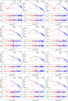 |
Fig. A.1 Top panel: simulated XMM-Newton (red) and NuSTAR (blue) spectra together with the various components of the theoretical model assumed. Primary emission plus ionized reflection (dashed lines), neutral reflection (dash dotted lines), and thermal emission (dotted lines) are indicated. Middle and bottom panels: the χ2 residuals obtained by the two blind fits (see Sect. 3.2 for details) are shown. |
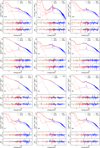 |
Fig. A.1 continued |
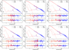 |
Fig. A.1 continued |
References
- Abbott, B. P., Abbott, R., Abbott, T. D., et al. 2016a, Phys. Rev. Lett., 116, 061102 [Google Scholar]
- Abbott, B. P., Abbott, R., Abbott, T. D., et al. 2016b, Phys. Rev. Lett., 116, 241103 [Google Scholar]
- Agol, E., & Krolik, J. H. 2000, ApJ, 528, 161 [NASA ADS] [CrossRef] [Google Scholar]
- Akaike, H. 1974, IEEE Trans. Autom. Control, 19, 716 [NASA ADS] [CrossRef] [MathSciNet] [Google Scholar]
- Arnaud, K. A. 1996, in Astronomical Data Analysis Software and Systems V, eds. G. H. Jacoby, & J. Barnes, ASP Conf. Ser., 101, 17 [NASA ADS] [Google Scholar]
- Bianchi, S., Guainazzi, M., Matt, G., Fonseca Bonilla, N., & Ponti, G. 2009, A&A, 495, 421 [NASA ADS] [CrossRef] [EDP Sciences] [Google Scholar]
- Blandford, R. D., & Znajek, R. L. 1977, MNRAS, 179, 433 [NASA ADS] [CrossRef] [Google Scholar]
- Bonson, K., & Gallo, L. C. 2016, MNRAS, 458, 1927 [NASA ADS] [CrossRef] [Google Scholar]
- Braito, V., Reeves, J. N., Gofford, J., et al. 2014, ApJ, 795, 87 [NASA ADS] [CrossRef] [Google Scholar]
- Brenneman, L. W., & Reynolds, C. S. 2006, ApJ, 652, 1028 [NASA ADS] [CrossRef] [Google Scholar]
- Brenneman, L. W., Reynolds, C. S., Nowak, M. A., et al. 2011, ApJ, 736, 103 [NASA ADS] [CrossRef] [Google Scholar]
- Capellupo, D. M., Netzer, H., Lira, P., Trakhtenbrot, B., & Mejía-Restrepo, J. 2015, MNRAS, 446, 3427 [NASA ADS] [CrossRef] [Google Scholar]
- Capellupo, D. M., Netzer, H., Lira, P., Trakhtenbrot, B., & Mejía-Restrepo, J. 2016, MNRAS, 460, 212 [NASA ADS] [CrossRef] [Google Scholar]
- Chartas, G., Kochanek, C. S., Dai, X., Poindexter, S., & Garmire, G. 2009, ApJ, 693, 174 [NASA ADS] [CrossRef] [Google Scholar]
- Choudhury, K., Garcia, J. A., Steiner, J. F., & Bambi, C. 2017, ApJ, 851, 57 [NASA ADS] [CrossRef] [Google Scholar]
- Collinson, J. S., Ward, M. J., Landt, H., et al. 2017, MNRAS, 465, 358 [NASA ADS] [CrossRef] [Google Scholar]
- Dauser, T., Wilms, J., Reynolds, C. S., & Brenneman, L. W. 2010, MNRAS, 409, 1534 [NASA ADS] [CrossRef] [Google Scholar]
- Dauser, T., Garcia, J., Wilms, J., et al. 2013, MNRAS, 430, 1694 [NASA ADS] [CrossRef] [Google Scholar]
- Dauser, T., García, J., Walton, D. J., et al. 2016, A&A, 590, A76 [NASA ADS] [CrossRef] [EDP Sciences] [Google Scholar]
- De Marco, B., Ponti, G., Cappi, M., et al. 2013, MNRAS, 431, 2441 [NASA ADS] [CrossRef] [Google Scholar]
- Done, C., Jin, C., Middleton, M., & Ward, M. 2013, MNRAS, 434, 1955 [NASA ADS] [CrossRef] [Google Scholar]
- Dovčiak, M., & Done, C. 2016, Astron. Nachr., 337, 441 [NASA ADS] [CrossRef] [Google Scholar]
- Dovčiak, M., Karas, V., & Yaqoob, T. 2004, ApJS, 153, 205 [NASA ADS] [CrossRef] [Google Scholar]
- Emmanoulopoulos, D., McHardy, I. M., & Papadakis, I. E. 2011, MNRAS, 416, L94 [NASA ADS] [CrossRef] [Google Scholar]
- Emmanoulopoulos, D., Papadakis, I. E., Dovčiak, M., & McHardy, I. M. 2014, MNRAS, 439, 3931 [NASA ADS] [CrossRef] [Google Scholar]
- Fabian, A. C. 2012, ARA&A, 50, 455 [NASA ADS] [CrossRef] [Google Scholar]
- Fabian, A. C., Rees, M. J., Stella, L., & White, N. E. 1989, MNRAS, 238, 729 [NASA ADS] [CrossRef] [Google Scholar]
- Fabian, A. C., Iwasawa, K., Reynolds, C. S., & Young, A. J. 2000, PASP, 112, 1145 [NASA ADS] [CrossRef] [Google Scholar]
- Fabian, A. C., Zoghbi, A., Ross, R. R., et al. 2009, Nature, 459, 540 [NASA ADS] [CrossRef] [PubMed] [Google Scholar]
- Fabian, A. C., Parker, M. L., Wilkins, D. R., et al. 2014, MNRAS, 439, 2307 [NASA ADS] [CrossRef] [Google Scholar]
- Fabian, A. C., Lohfink, A., Kara, E., et al. 2015, MNRAS, 451, 4375 [NASA ADS] [CrossRef] [Google Scholar]
- Foreman-Mackey, D. 2016, J. Open Source Softw., 24 [Google Scholar]
- Gallo, L. C., Wilkins, D. R., Bonson, K., et al. 2015, MNRAS, 446, 633 [NASA ADS] [CrossRef] [Google Scholar]
- Gammie, C. F., Shapiro, S. L., & McKinney, J. C. 2004, ApJ, 602, 312 [NASA ADS] [CrossRef] [Google Scholar]
- García, J., Dauser, T., Reynolds, C. S., et al. 2013, ApJ, 768, 146 [NASA ADS] [CrossRef] [Google Scholar]
- García, J., Dauser, T., Lohfink, A., et al. 2014, ApJ, 782, 76 [NASA ADS] [CrossRef] [Google Scholar]
- George, I. M.,& Fabian, A. C. 1991, MNRAS, 249, 352 [NASA ADS] [CrossRef] [Google Scholar]
- Ghisellini, G., Haardt, F., & Matt, G. 1994, MNRAS, 267, 743 [NASA ADS] [CrossRef] [Google Scholar]
- Gierliński, M., Middleton, M., Ward, M., & Done, C. 2008, Nature, 455, 369 [NASA ADS] [CrossRef] [PubMed] [Google Scholar]
- Gofford, J., Reeves, J. N., McLaughlin, D. E., et al. 2015, MNRAS, 451, 4169 [Google Scholar]
- Goodman, J., & Weare, J. 2010, Comm. App. Math. Comp. Sci., 5, 65 [Google Scholar]
- Grevesse, N., & Sauval, A. J. 1998, Space Sci. Rev., 85, 161 [NASA ADS] [CrossRef] [Google Scholar]
- Guainazzi, M., Bianchi, S., & Dovčiak M. 2006, Astron. Nachr., 327, 1032 [NASA ADS] [CrossRef] [Google Scholar]
- Haardt, F., & Maraschi, L. 1993, ApJ, 413, 507 [NASA ADS] [CrossRef] [MathSciNet] [Google Scholar]
- Harrison, F. A., Craig, W. W., Christensen, F. E., et al. 2013, ApJ, 770, 103 [NASA ADS] [CrossRef] [Google Scholar]
- Hunter, J. D. 2007, Comput. Sci. Eng., 9, 90 [Google Scholar]
- Jansen, F., Lumb, D., Altieri, B., et al. 2001, A&A, 365, L1 [NASA ADS] [CrossRef] [EDP Sciences] [Google Scholar]
- Kallman, T., & Bautista, M. 2001, ApJS, 133, 221 [NASA ADS] [CrossRef] [Google Scholar]
- Kammoun, E. S., & Papadakis, I. E. 2017, MNRAS, 472, 3131 [NASA ADS] [CrossRef] [Google Scholar]
- Kara, E., Alston, W. N., Fabian, A. C., et al. 2016, MNRAS, 462, 511 [Google Scholar]
- Kerr, R. P. 1963, Phys. Rev. Lett., 11, 237 [NASA ADS] [CrossRef] [MathSciNet] [Google Scholar]
- King, A. R., Pringle, J. E., & Hofmann, J. A. 2008, MNRAS, 385, 1621 [NASA ADS] [CrossRef] [Google Scholar]
- King, A. L., Miller, J. M., Bietenholz, M., et al. 2015, ApJ, 799, L8 [NASA ADS] [CrossRef] [Google Scholar]
- Laor, A. 1991, ApJ, 376, 90 [NASA ADS] [CrossRef] [Google Scholar]
- Lightman, A. P., & White, T. R. 1988, ApJ, 335, 57 [NASA ADS] [CrossRef] [Google Scholar]
- Mantovani, G., Nandra, K., & Ponti, G. 2016, MNRAS, 458, 4198 [NASA ADS] [CrossRef] [Google Scholar]
- Matt, G., Guainazzi, M., & Maiolino, R. 2003, MNRAS, 342, 422 [NASA ADS] [CrossRef] [Google Scholar]
- McHardy, I. M., Koerding, E., Knigge, C., Uttley, P., & Fender, R. P. 2006, Nature, 444, 730 [NASA ADS] [CrossRef] [PubMed] [Google Scholar]
- McKinney, J. C., & Gammie, C. F. 2004, ApJ, 611, 977 [NASA ADS] [CrossRef] [Google Scholar]
- Miller, L., Turner, T. J., & Reeves, J. N. 2008, A&A, 483, 437 [NASA ADS] [CrossRef] [EDP Sciences] [Google Scholar]
- Miller, L., Turner, T. J., & Reeves, J. N. 2009, MNRAS, 399, L69 [NASA ADS] [CrossRef] [Google Scholar]
- Miniutti, G., & Fabian, A. C. 2004, MNRAS, 349, 1435 [NASA ADS] [CrossRef] [Google Scholar]
- Mohan, P., & Mangalam, A. 2014, ApJ, 791, 74 [CrossRef] [Google Scholar]
- Mosquera, A. M., Kochanek, C. S., Chen, B., et al. 2013, ApJ, 769, 53 [NASA ADS] [CrossRef] [Google Scholar]
- Nandra, K., Barret, D., Barcons, X., et al. 2013, ArXiv e-prints [arXiv: 1306.2307] [Google Scholar]
- Nardini, E., Gofford, J., Reeves, J. N., et al. 2015, MNRAS, 453, 2558 [NASA ADS] [CrossRef] [Google Scholar]
- Parker, M. L., Miller, J. M., & Fabian, A. C. 2017, MNRAS, 474, 1538 [Google Scholar]
- Patrick, A. R., Reeves, J. N., Lobban, A. P., Porquet, D., & Markowitz, A. G. 2011, MNRAS, 416, 2725 [NASA ADS] [CrossRef] [Google Scholar]
- Petrucci, P. O., Haardt, F., Maraschi, L., et al. 2001a, ApJ, 556, 716 [NASA ADS] [CrossRef] [Google Scholar]
- Petrucci, P. O., Merloni, A., Fabian, A., Haardt, F., & Gallo, E. 2001b, MNRAS, 328, 501 [NASA ADS] [CrossRef] [Google Scholar]
- Rau, A., Meidinger, N., Nandra, K., et al. 2013, ArXiv e-prints [arXiv: 1308.6785] [Google Scholar]
- Reis, R. C., & Miller, J. M. 2013, ApJ, 769, L7 [Google Scholar]
- Reynolds, C. S. 2014, Space Sci. Rev., 183, 277 [Google Scholar]
- Reynolds, C. S., & Nowak, M. A. 2003, Phys. Rep., 377, 389 [NASA ADS] [CrossRef] [Google Scholar]
- Reynolds, C. S., Brenneman, L. W., Lohfink, A. M., et al. 2012, ApJ, 755, 88 [NASA ADS] [CrossRef] [Google Scholar]
- Risaliti, G. 2016, Astron. Nachr., 337, 529 [NASA ADS] [CrossRef] [Google Scholar]
- Risaliti, G., Elvis, M., Fabbiano, G., et al. 2007, ApJ, 659, L111 [NASA ADS] [CrossRef] [Google Scholar]
- Risaliti, G., Harrison, F. A., Madsen, K. K., et al. 2013, Nature, 494, 449 [NASA ADS] [CrossRef] [Google Scholar]
- Shapiro, S. L., Lightman, A. P., & Eardley, D. M. 1976, ApJ, 204, 187 [NASA ADS] [CrossRef] [Google Scholar]
- Smith, K. Z., Acton, D. S., Gallagher, B. B., et al. 2016, in Space Telescopes and Instrumentation: Optical, Infrared, and Millimeter Wave, Proc. SPIE, 9904, 990442 [CrossRef] [Google Scholar]
- Steiner, J. F., García, J. A., Eikmann, W., et al. 2017, ApJ, 836, 119 [NASA ADS] [CrossRef] [Google Scholar]
- Strüder, L., Briel, U., Dennerl, K., et al. 2001, A&A, 365, L18 [NASA ADS] [CrossRef] [EDP Sciences] [Google Scholar]
- Tatum, M. M., Turner, T. J., Miller, L., & Reeves, J. N. 2013, ApJ, 762, 80 [NASA ADS] [CrossRef] [Google Scholar]
- Thorne, K. S. 1974, ApJ, 191, 507 [Google Scholar]
- Vasudevan, R. V., Fabian, A. C., Reynolds, C. S., et al. 2016, MNRAS, 458, 2012 [NASA ADS] [CrossRef] [Google Scholar]
- Vaughan, S., & Uttley, P. 2005, MNRAS, 362, 235 [NASA ADS] [CrossRef] [Google Scholar]
- Vaughan, S., & Uttley, P. 2006, Adv. Space Res., 38, 1405 [NASA ADS] [CrossRef] [Google Scholar]
- Volonteri, M., Sikora, M., Lasota, J.-P., & Merloni, A. 2013, ApJ, 775, 94 [NASA ADS] [CrossRef] [Google Scholar]
- Walton, D. J., Nardini, E., Fabian, A. C., Gallo, L. C., & Reis, R. C. 2013, MNRAS, 428, 2901 [NASA ADS] [CrossRef] [Google Scholar]
- Walton, D. J., Risaliti, G., Harrison, F. A., et al. 2014, ApJ, 788, 76 [NASA ADS] [CrossRef] [Google Scholar]
- Yaqoob, T. 2012, MNRAS, 423, 3360 [NASA ADS] [CrossRef] [Google Scholar]
ξ = L∕nr2 is the ionization parameter (units erg cm s−1), where L is the luminosity of the X-ray source, and n is the volume density of the absorber situated at a distance r from the source.
This is approximately the maximum effective exposure per XMM-Newton orbit in Small Window mode (needed to avoid pile-up in bright sources).
We use the XSPEC_EMCEE implementation of the PYTHON EMCEE package for X-ray spectral fitting in XSPEC by Jeremy Sanders (http://github.com/jeremysanders/xspec_emcee).
We note that we considered the ratios ξfit∕ξinput for the ionization parameters of the accretion disc (ξd) and of the warm absorber (ξwa) rather than the ratios of the logarithms.
All Tables
Key parameters used to perform the simulations with the corresponding input range, for the various emission and absorption components.
Summary of the success/failure in measuring the relevant parameters for the three simulation sets.
Summary of the constraints on determining the spin showing its dependence on the lamp-post height.
Input and best-fit values of the height (h) and the spin parameter (a*) found for the two fits performed to the spectra of Sets G, K, and B.
All Figures
|
Fig. 1 Schematic (not to scale) of the proposed configuration, presenting the various emission and absorption features that we consider in this work (see Sect. 3.1 for details). |
| In the text | |
|
Fig. 2 Toppanel: example of the simulated XMM-Newton (red) and NuSTAR (blue) spectra (corresponding to simulation G8) together with the various components of the theoretical model assumed. The primary emission plus ionized reflection (dashed lines), neutral reflection (dash-dotted lines), and thermal emission (dotted lines) are shown. Middle and bottom panels: the χ2 residuals obtained by the two separate fits are indicated (see Sect. 3.2 for details). |
| In the text | |
|
Fig. 3 Results of the MCMC analysis for the relevant best-fit reflection parameters corresponding to the two different spectral fits shown in the middle and bottom panels of Fig. 2. The red lines correspond to the input values assumed in order to create the simulations. We show the χ2 values obtained from the corresponding best fit, whose accuracy as a whole is excellent in both cases. The individual parameters, however, are not all correctly retrieved. |
| In the text | |
|
Fig. 4 Input values (black dots) of the reflection parameters assumed for creating the various simulations (for Set G). The best-fit values obtained for the various parameters are shown as squares and diamonds for the two different realizations. The colour code refers to the quality of the fit as a whole: green for excellent, yellow for good, and red for inaccurate (see text for details). The error bars represent the 90% confidence levels obtained from the MCMC analysis. |
| In the text | |
|
Fig. 5 Similar to Fig. 4 but for the absorption parameters (top panels) and the gas temperature of thermal emission component (last panel), presenting the results for sets G and K. The column densities are in units of 1022 cm −2. |
| In the text | |
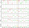 |
Fig. 6 Similar to Fig. 4 but for Sets K and B. |
| In the text | |
|
Fig. 7 Distribution of spin measurements from Vasudevan et al. (2016) (blue histograms) and the distribution of wrong and undetermined measurements (red histograms) obtained from the simulations performed in the current work. |
| In the text | |
|
Fig. 8 Black hole spin vs. lamp-post height contour plots obtained by the MCMC analysis obtained from the best-spectral fits of G6 (top panel) and G11 (bottom panel), performed using the Athena-WFI response files. The input spin and height values (red lines) are listed on the top right corner of each panel for the corresponding simulation. |
| In the text | |
|
Fig. A.1 Top panel: simulated XMM-Newton (red) and NuSTAR (blue) spectra together with the various components of the theoretical model assumed. Primary emission plus ionized reflection (dashed lines), neutral reflection (dash dotted lines), and thermal emission (dotted lines) are indicated. Middle and bottom panels: the χ2 residuals obtained by the two blind fits (see Sect. 3.2 for details) are shown. |
| In the text | |
|
Fig. A.1 continued |
| In the text | |
|
Fig. A.1 continued |
| In the text | |
Current usage metrics show cumulative count of Article Views (full-text article views including HTML views, PDF and ePub downloads, according to the available data) and Abstracts Views on Vision4Press platform.
Data correspond to usage on the plateform after 2015. The current usage metrics is available 48-96 hours after online publication and is updated daily on week days.
Initial download of the metrics may take a while.