© ESO 2018

1 Introduction

The motivation of the present study was to modify and generalize the known method for analyzing anisotropic flow in relativistic nuclear collisions (Voloshin & Zhang 1996; Poskanzer & Voloshin 1998), which has been effectively applied in many studies, for example, recently in Adam et al. (2016). The method is based on the use of the Fourier expansion of azimuthal distributions of produced particles and allows us to obtain important information on the mechanism of nuclear collisions. However, mathematical formalism of this method is more general and can be used after minor modifications even for quite different kinds of analysis. Our present idea is focused primarily on astrometry. Recently, some similarity between spiral structures in galactic patterns and heavy ion collisions has been discussed (Rustamov & Rustamov 2016). However, our approach is different. We make use of the formalism of the Fourier analysis of nuclear collisions simply as a tool and we do not consider a common physics that could bridge the two different fields. Moreover, Fourier analysis is only one of two methods that we work with.

In our approach the astrometric data are decomposed into a set of limited, finite star patterns whose parameters are statistically analyzed. These parameters define characteristics of the patterns and represent statistical deviations from the uniform distribution of stars; for example, a tendency to display scale-dependent clustering or anti-clustering. The aim is to find and interpret these deviations. The input data are taken from the Gaia DR1 catalog (Gaia Collaboration 2016b,a).

In Sect. 2.1 we define some useful terms and explain the essence of our task in more detail. The general description of the Fourier analysis modified for application to astrometry is presented in Sect. 2.2. Then in Sect. 2.3 we describe a complementary statistical method for analysis of the patterns of stars, which deals with angular distances and is important for identification of binary and ternary star systems. The results obtained from the application of both methods to the Gaia data are presented and discussed in Sect. 3.1. A discussion on the gravitational microlensing effect and the conditions of its observation is given in Sect. 3.2. A brief summary of the paper is presented in Sect. 4.

2 Methods

2.1 Subject of analysis

Let us consider a region of the sphere of the galactic reference frame. We study the patterns of the stars inside the circles of the same angular radius as in Fig. 1a that cover the chosen region. The circular shape is essential for application of our methods and the stars among the circles are not used for statistical analysis. First, in accordance with the figure, we define one event of the multiplicity M as a set of stars with angular positions $\left\{l_i,b_i\right\},i=1,\mathrm{...}M$ inside one circle with the center (l₀, b₀) and a small angular radius ρ (introduced terms are inspired by particle physics). The letter l(b) represents the galactic longitude (latitude). The positions inside the circle (event) can be represented equivalently by the three-dimensional (3D) unit vectors n_α as sketched in Fig. 1b: $$n_{\alpha }=(\cos b_{\alpha }\cos l_{\alpha },\cos b_{\alpha }\sin l_{\alpha },\sin b_{\alpha }),\alpha =0,\mathrm{...}M.$$(1)

Subsequently, the event can be defined as the set of stars meeting the condition: $$\left|n_i-n_0\right|\le \rho ,i=1,\mathrm{...}M.$$(2)

One can define for each event its local orthonormal frame defined on the basis: 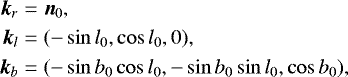$$\begin{array}{ll}{k}_r\hfill & =n_0,\hfill \\ k_l\hfill & =(-\sin l_0,\cos l_0,0),\hfill \\ k_b\hfill & =(-\sin b_0\cos l_0,-\sin b_0\sin l_0,\cos b_0),\hfill \end{array}$$(3)

where k_l(k_b) represent local directions of the longitude (latitude). The local coordinates are defined as $$x_i=n_i^{\prime }.k_l,y_i=n_i^{\prime }.k_b;n_i^{\prime }=n_i-n_0.$$(4)

We work with the following representations of the star positions (Fig. 3a) inside the event circle:

1) Two-dimensional (2D) positions {x_i, y_i} (Sect. 2.3): $$\{x_i,y_i\};x_i^2+y_i^2\le {\rho }^2,i=1,\mathrm{...}M.$$(5)

2) Azimuthal positions $\left\{{\phi }_i\right\}$ (Sect. 2.2): $$\left\{{\phi }_i\right\};-\pi <{\phi }_i<\pi ,i=1,\mathrm{...}M,$$(6)

defined by x_i, y_i: $$x_i=r_i\cos {\phi }_i,y_i=r_i\sin {\phi }_i,r_i=\sqrt{x_i^2+y_i^2}.$$(7)

Here we use two sources of input data: (A) The simulated events generated by the Monte-Carlo (MC) code; Fig. 1a is an example of uniform generation of the star positions, and (B) the real star events obtained from the Gaia catalog. The methods for their analysis are described below. The final results of the analysis follow from the comparison of the parameters and distributions obtained from both sources of input data.

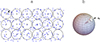Fig. 1 Patterns of the stars inside the grid of circles (a). Position n0 of the event defines its local reference frame (b).

2.2 Fourier analysis

We start from the general formalism introduced in Voloshin & Zhang (1996) and Poskanzer & Voloshin (1998). The angular distribution P(φ) > 0 in (−π, π) can be expressed as the Fourier series $$\begin{array}{l}P(\phi )=\frac{1}{2\pi }\left(1+2{\sum }_{n=1}^{\infty }{v}_n\cos \left[n\left(\phi -{\Psi }_n\right)\right]\right),\\ {\displaystyle {\int }_{-\pi }^{\pi }P}(\phi )\text{d}\phi =1,\end{array}$$(8)

where the set of parameters $\left\{v_n,{\Psi }_n\right\}$ define the distribution. If we define the mean value of the function f as 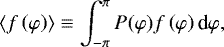$$\langle f\left(\phi \right)\rangle \equiv {\displaystyle {\int }_{-\pi }^{\pi }P}(\phi )f\left(\phi \right)\text{d}\phi ,$$(9)

then the orthogonality of the terms in Eq. (8) implies: $$\begin{array}{l}{v}_n=\langle \cos \left[n\left(\phi -{\Psi }_n\right)\right]\rangle ,\\ \tan \left(n{\Psi }_n\right)=\frac{\langle \sin \left(n\phi \right)\rangle }{\langle \cos \left(n\phi \right)\rangle },\end{array}$$

for any n = 1, 2, 3, ... If we take event (6) in which the probability of φ_i is proportional to P(φ_i) and replace the average value defined by Eq. (9) with the summation 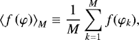$${\langle f\left(\phi \right)\rangle }_M\equiv \frac{1}{M}{\sum }_{k=1}^{M}f({\phi }_k),$$(12)

then insteadof Eqs. (10) and (11) we get $$\begin{array}{l}{v}_n(M)={\langle \cos \left[n\left(\phi -{\Psi }_n\right)\right]\rangle }_M,\\ \tan \left(n{\Psi }_n(M)\right)=\frac{{\langle \sin \left(n\phi \right)\rangle }_M}{{\langle \cos \left(n\phi \right)\rangle }_M}.\end{array}$$

Apparently, for any n = 1, 2, 3, ... and M →∞ one can expect: $${\langle f\left(\phi \right)\rangle }_M\to \langle f\left(\phi \right)\rangle ,v_n(M)\to v_n,{\Psi }_n(M)\to {\Psi }_n.$$(15)

The Eqs. (13) and (14) do not have an unambiguous solution, as illustrated in Fig. 2.

The panels represent distributions $$P(\psi )=1+2v_n\cos (n\psi ),\psi =\phi -{\Psi }_n.$$(16)

The relation in Eq. (14) gives the solutions $$n{\Psi }_n(M)={\tan }^{-1}\left[\frac{{\langle \sin \left(n\phi \right)\rangle }_M}{{\langle \cos \left(n\phi \right)\rangle }_M}\right]+k\pi .$$(17)

The sign of the term $v_n\cos \left[n\left(\phi -{\Psi }_n\right)\right]$ in Eq. (8) can be controlled either by the sign of v_n or by the phase nΨ_n. Apparently the change v_n →−v_n is equivalent to nΨ _n → nΨ_n ± kπ, k = 1, 2, 3, ... Nevertheless in the present paper we analyze only $v_n^2(M)$ and not v_n(M) with the phase Ψ_n(M). Therefore the sign ambiguity does not play a role.

The relation in Eq. (13) implies $$v_n(M)=\cos \left(n{\Psi }_n\right){\langle \cos \left(n\phi \right)\rangle }_M+\sin \left(n{\Psi }_n\right){\langle \sin \left(n\phi \right)\rangle }_M.$$(18)

The relations $$\sin x=\frac{\tan x}{\sqrt{1+{\tan }^{2}x}},\cos x=\frac{1}{\sqrt{1+{\tan }^{2}x}},$$(19)

together with Eq. (14) give $$\begin{array}{ll}\sin \left(n{\Psi }_n\right)\hfill & =\frac{{\langle \sin \left(n\phi \right)\rangle }_M}{\sqrt{{\langle \cos \left(n\phi \right)\rangle }_M^2+{\langle \sin \left(n\phi \right)\rangle }_M^2}},\hfill \\ \cos \left(n{\Psi }_n\right)\hfill & =\frac{{\langle \cos \left(n\phi \right)\rangle }_M}{\sqrt{{\langle \cos \left(n\phi \right)\rangle }_M^2+{\langle \sin \left(n\phi \right)\rangle }_M^2}}.\hfill \end{array}$$

Inserting of these latter two expressions into Eq. (18) after some algebra gives $$v_n^2(M)={\langle \cos \left(n\phi \right)\rangle }_M^2+{\langle \sin \left(n\phi \right)\rangle }_M^2.$$(22)

We note that $v_n^2$ does not depend on the choice of k in Eq. (17). The last relation can be modified as $$v_n^2(M)=\frac{1}{M}\left[1+\frac{2}{M}{\sum }_{1\le k<l\le M}\cos (n{\phi }_k-n{\phi }_l)\right].$$(23)

There are two extreme cases:

1) All angles are in a narrow cone so that cos(nφ_i − nφ_j) ≈ 1; subsequently $${\sum }_{1\le k<l\le M}\cos (n{\phi }_k-n{\phi }_l)\approx \frac{M(M-1)}{2},$$(24)

and $$v_n^2(M)\approx 1.$$(25)

2) All angles are regularly distributed on the circle, so φ_k = 2πk∕M (anti-clustering). If we define q = exp(i2πn∕M), n∕M≠1, 2, 3, ..., then we get $$\begin{array}{ll}{\sum }_{1\le k<l\le M}\cos (n{\phi }_k-n{\phi }_l)\hfill & =\mathrm{Re}{\sum }_{1\le k<l\le M}{q}^{k-l}\hfill \\ \hfill & =-\mathrm{Re}\frac{q\left[1+M\left(q-1\right)-q^M\right]}{{\left(q-1\right)}^2}\hfill \\ \hfill & =M\mathrm{Re}\frac{q}{1-q}=-\frac{M}{2},\hfill \end{array}$$(26)

which after inserting to Eq. (23) gives $$v_n^2(M)=0.$$(27)

This result confirms an expectation that the regular distribution should not generate asymmetry terms in Eq. (8). In general, we can have N_M events of the same multiplicity M $$-\pi \le {\theta }_j-\Delta \le {\phi }_1^j,\mathrm{..},{\phi }_M^j\le {\theta }_j+\Delta \le \pi ,j=1,\mathrm{..}{N}_M,$$(28)

where θ_j can be different for various events. Subsequently, the average value of $v_n^2(M)$ defined by Eq. (23) can be estimated as $$\langle v_n^2(M)\rangle =\frac{1}{M}\left[1+\frac{2}{M}{\sum }_{1\le k<l\le M}\langle \cos (n{\phi }_k^j-n{\phi }_l^j)\rangle \right],$$(29)

where $$\langle \cos (n{\phi }_k^j-n{\phi }_l^j)\rangle =\frac{1}{N_M}{\sum }_{j=1}^{N_M}\cos (n{\phi }_k^j-n{\phi }_l^j).$$(30)

For uniform distribution of ${\phi }_k^j$ inside the intervals of Eq. (28), and with sufficiently great N_M, one can estimate this value by the integral $$\begin{array}{l}\langle \cos (n\phi -n\psi )\rangle \\ =\frac{1}{4{\Delta }^2}{\displaystyle {\int }_{-\Delta }^{\Delta }{\displaystyle {\int }_{-\Delta }^{\Delta }\left(\cos n\phi \cos n\psi +\sin n\phi \sin n\psi \right)}}\text{d}\phi \text{d}\psi \\ ={\left(\frac{\sin n\Delta }{n\Delta }\right)}^2.\end{array}$$(31)

Subsequently, for any n = 1, 2, 3, ... we have $$\langle v_n^2(M)\rangle =\frac{1}{M}\left[1+\left(M-1\right){\left(\frac{\sin n\Delta }{n\Delta }\right)}^2\right]\ge \frac{1}{M},$$(32)

and therefore for Δ → 0 (clustering), we obtain $$\langle v_n^2(M)\rangle \to 1,$$(33)

which corresponds to case (I) of Eq. (24). For Δ = π (uniform distribution) one obtains $$\langle v_n^2(M)\rangle =\frac{1}{M}.$$(34)

To explain the practical meaning of the relation in Eq. (33), let us assume the stars inside the circle in Fig. 3a are not distributed uniformly over this circle, but are concentrated in some smaller circle, which is located anywhere inside the greater one in Fig. 3b; their positions $\left\{{\phi }_1\mathrm{...}{\phi }_M\right\}$ inside the greater circle fill up a narrower angular segment (statistically). Such a scenario is reflected in Eqs. (25) and (33). In general there can be a mixture uniform + clustering, something between (33) and (34): $$\frac{1}{M}<\langle v_n^2\left(M\right)\rangle <1.$$(35)

Furthermore, the relation in Eq. (34) corresponds to the uniform distribution, and for M →∞ gives $$\langle v_n^2(M)\rangle \to 0,$$(36)

which is thecorrect result for uniform distribution defined by Eq. (8). But why does a finite M generate $\langle v_n^2(M)\rangle >0$ even for uniform generation? The reason is that the event of finite multiplicity, for example M = 3 of random stars, is usually better described with the use of higher harmonics. For increasing M the population becomes denser and more symmetric in terms of $\left\{{\phi }_1\mathrm{...}{\phi }_M\right\}$, in accordance with Eq. (36).

Here we also use the function Θ_n defined as $${\Theta }_n(M)=M\langle v_n^2(M)\rangle .$$(37)

For illustration we present the toy examples of simulation:

a) Uniform distribution

We generate uniform sets of stars inside the circle of radius ρ, like the event in Fig. 3a.

For each event we use the relation in Eq. (22) to calculate $v_n^2(M)$ for n = 1, 2, 3. The functions $${\Theta }_n(M)=M\langle v_n^2(M)\rangle =\frac{M}{N_M}{\sum }_{k=1}^{N_M}{v}_{n,k}^2(M),$$(38)

where N_M is the number of events of multiplicity M, are displayed in the upper panels of Fig. 4. The resulting lines appa- rently satisfy Eq. (34). We note that throughout the paper, the error bars, if plotted, indicate only statistical errors.

b) Clustering

In a first step, we uniformly generate stars inside a smaller circle of radius δ. This circle is randomly located inside the greater circle of radius ρ, and we define λ = δ∕ρ (Fig. 3b). The functions Θ_n(ρ, δ, M) are calculated with the use of Eq. (38), equally as in the previous case. The results are displayed in the middle panels of Fig. 4.

c) Anti-clustering

We generate spots of the radius δ inside the circle of radius ρ, giving the ratio λ = δ∕ρ (Fig. 3c). The MC algorithm is the same as for uniform distribution, but with the additional constraint that the spots must not overlap. If two spots in uniform generation overlap, one of them is excluded. In other words, there is a rule that the distance between any two stars is greater than 2δ. The corresponding functions (38) are displayed in the lower panels of Fig. 4. Why do the curves decrease? Obviously, a denser population of spots inside the circle generates a more regular arrangement of φ_k, closer to case (II) above, so the function Θ_n(M) will tend to approach the minimum given by Eq. (27). The curves in the figure are linear for a small λ and M ≪ M_max ≲ 1∕λ² and one can approximate as $${\Theta }_n(\rho ,\delta ,M)\approx 1-3.36{\lambda }^2\left(M-1\right),$$(39)

for n = 1, 2, 3.

Generally, for both algorithms mentioned above, the change of scale ρ → kρ, δ → kδ does not change distribution of angles in the event $\left\{{\phi }_1\mathrm{...}{\phi }_M\right\}$ and $\langle v_n^2(M)\rangle$ defined by Eq. (29); therefore $${\Theta }_n(\rho ,\delta ,M)={\Theta }_n(\lambda ,M);\lambda =\delta /\rho .$$(40)

These algorithms are simple examples; one could think up other ones.

We summarize the main results of this section as follows.

1) The uniform field (like the events in Fig. 1a) generate the dependence Θ _n (M) = 1 for any n = 1, 2, 3, ... The non-uniform distributions violate this rule. We have shown the examples, which generate relations Θ _n (M) > 1 (clustering) and Θ_n(M) < 1 (anti-clustering).

2) In this way the functions Θ_n(M) give important information about the statistical character of the patterns, but the numbers $v_n^2(M)$ calculated only from a single event do not offer a significant amount of information.

The functions Θ_n(M) are used in Sect. 3.1 for analysis and classification of the sets of real star events.

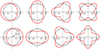Fig. 2 Examples of deviations from uniform angular distribution defined by Eq. (16). The red curves are their representation in polar coordinates (P(ψ), ψ) as indicated in the lower left panel. The panels from left to right correspond to n = 1, 2, 3, 4. The upper (lower) panels correspond to the negative (positive) sign of vn = ∓1∕6. The black dot-dashed circles correspond to uniform distribution P(ψ) = 1.

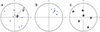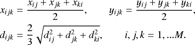
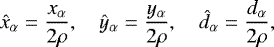
Fig. 3 Examples of the events generated by different algorithms: uniform distribution (a), clustering λ = 1∕3 (b), and anti-clustering λ = 1∕20 (c).

2.3 Distributions of angular distances

Inside event (5) we define the angular distances: $$x_{ij}=\left|x_i-x_j\right|,y_{ij}=\left|y_i-y_j\right|,d_{ij}=\sqrt{x_{ij}^2+y_{ij}^2}.$$(41)

We also define the parameters characterizing the dimension of a triplet of stars: $$\begin{array}{ll}{x}_{ijk}\hfill & =\frac{x_{ij}+x_{jk}+x_{ki}}{2},y_{ijk}=\frac{y_{ij}+y_{jk}+y_{ki}}{2},\hfill \\ d_{ijk}\hfill & =\frac{2}{3}\sqrt{d_{ij}^2+d_{jk}^2+d_{ki}^2},i,j,k=1,\mathrm{...}M.\hfill \end{array}$$(42)

Let us consider a uniform field of stars (Fig. 1a). The example of a single event (5) is displayed in Fig. 3a. For the set of events we can calculate probability distributions of the parameters defined above. The distributions satisfy:

1) The shape of the (normalized) distribution of y_ij is the same as that of x_ij; similarly for x_ijk and y_ijk. Therefore for the uniform events, there are four different distributions, $$P_1(x_{ij},\rho ),P_2(d_{ij},\rho ),P_3(x_{ijk},\rho ),P_4(d_{ijk},\rho ).$$(43)

2) The shapes of these distributions do not depend on multiplicity. Since the numbers x_j are independent, the distribution of x_jk is the same for any j, k. Increasing M means only greater density, that is, greater numbers of x_j and x_jk, but proportion between different scales of x_jk does not change. The same argument holds for the distribution of all the parameters (Eqs. (41),(42)).

3) Obviously, there is the similarity P(Δ, ρ) ~ P(kΔ, kρ) for the distributions above, Δ = x_α, y_α, d_α. If we rescalethe distance parameters as $${\widehat{x}}_{\alpha }=\frac{x_{\alpha }}{2\rho },{\widehat{y}}_{\alpha }=\frac{y_{\alpha }}{2\rho },{\widehat{d}}_{\alpha }=\frac{d_{\alpha }}{2\rho },$$(44)

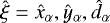then one can check that $0\le \widehat{\xi }\le 1$ for $\widehat{\xi }={\widehat{x}}_{\alpha },{\widehat{y}}_{\alpha },{\widehat{d}}_{\alpha }$ and α =ij or α =ijk. The corresponding normalized MC distributions $P\left(\widehat{\xi }\right)$ are together with the corresponding 3D plots $P\left({\widehat{x}}_{\alpha },{\widehat{y}}_{\alpha }\right)$ displayed in Fig. 5. These distributions can be approximated by the function 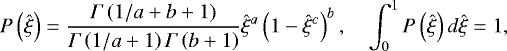$$P\left(\widehat{\xi }\right)=\frac{\Gamma \left(1/a+b+1\right)}{\Gamma \left(1/a+1\right)\Gamma \left(b+1\right)}{\widehat{\xi }}^a{\left(1-{\widehat{\xi }}^c\right)}^b,{\displaystyle {\int }_0^{1}P}\left(\widehat{\xi }\right)d\widehat{\xi }=1,$$(45)

where the parameters a, b, c optimized by the fits in the whole region $0<\widehat{\xi }<1$ are listed in Table 1.

The universal plots in the figure, after rescaling $\widehat{\xi }\to \Delta =2\rho \widehat{\xi }$, will serve in the following section as the templates for comparison with the real events of angular radius ρ. We must point out that the functions Eq. (45) with the parameters in the table are only approximations of the MC distributions. The very good agreement in Fig. 5 is due to “flexibility” of this parameterization, which for a, b, c ≥ 0 satisfies needed boundary conditions: $P\left(\widehat{\xi }\right)\to 0$ for $\widehat{\xi }\to 0$ and $\widehat{\xi }\to 1$. The term with the Γ−functions provides normalization. Despite the simple MC algorithm for the definition of the distributions $P\left(\widehat{\xi }\right)$, we did not succeed in expressing their exact form in terms of the known standard or special functions. However, in principle we can calculate them with arbitrary precision, which is needed for the data analysis. We refer to the following rules of the MC technique. The statistical error of a simulated distribution in the kth bin is $\approx 1/\sqrt{n_k}$, where n_k is bin population. For an accurate analysis, this error should be much less than the statistical error in the corresponding bin of the real data. In other words, the number of simulated events should be substantially greater than the number of the corresponding data events. In general, the precision of simulated distributions increases with the number of generated events.

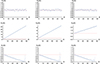Fig. 4 The functions Θn(M), n = 1, 2, 3 for Monte-Carlo events in the scenario of uniform distribution (upper panels). The remaining panels show clustering λ = 1∕3 (middle panels) and anti-clustering scenarios λ = 1∕20 (lower panels). Each multiplicity bin is generated by NM = 6000 events. The red lines correspond to the expected dependence for uniform distribution, Θ n (M) = 1 (Eq. (34)).

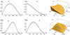Fig. 5 Distributions of angular distances $P({\widehat{x}}_{\alpha })$ of uniformly generated stars (points) fitted by the red curves (Eq. (45)). Corresponding distribution $P({\widehat{x}}_{\alpha },{\widehat{y}}_{\alpha })$ is on the right. Variables in panels are defined by relations (41)–(44). The Monte-Carlo statistics is represented by 2.5 × 106 events of multiplicity M = 5.

Fig. 6 Analyzed regions in the Gaia catalog, where ρ is angular radius of the events, M is their multiplicity and Ne is the number of events. Analysis is done only for events 2 ≤ M ≤ 15.

3 Application to the Gaia mission data

3.1 Violation of uniformity and bound star systems

The simulations described above have been applied to the analysis of the data from the recent Gaia catalog DR1 Gaia Collaboration (2016a). We present the results from the regions marked in Fig. 6. In the present paper we are starting this analysis from the simplest case, from the events of a small multiplicity. This condition refers to the small but different event radii in regions C and N&S (table in Fig. 6). In general, the scale of the possible structure violating uniformity should be less than the event radius ρ.

First, we applied the Fourier analysis described in Sect. 2.2. The corresponding functions Θ _n (M) are shown in Fig. 7. The upper part corresponds to a dense region C and very similar results can be obtained over other regions at the galactic plane.

The result qualitatively corresponds to the scenario of anti-clustering simulated in the lower panels of Fig. 4, however the slope of Θ ₁ appears to differ from the slopes of Θ₂ and Θ ₃. The lower panels correspond to sparse region N&S and the slopes Θ_n(M) suggest the presence of clustering.

To better understand these results, we have carried out a further analysis with the method described in Sect. 2.3. In Fig. 8 we show distributions of angular distances studied in region C, where we work with the events of radius ρ = 0.005deg = 18′′, which means d_{ij max} = x_{ij max} = y_{ij max} = 36′′, as seen in panel d. For comparison with simulation of uniform events we used the variables ${\widehat{x}}_{ij},{\widehat{y}}_{ij},{\widehat{d}}_{ij}$ defined in Eq. (44). The MC curves are the same as in panels a and b of Fig. 5. For ${\widehat{d}}_{ij}\gtrsim 0.11$ (or equivalently d_ij ≳ 4′′) the data agree perfectly with the MC simulation. However, the perfect agreement expected for uniform events is violated for d_ij ≲ 4′′. In fact we observe a 2D representation of the effect reported in (Arenou et al. 2017; Sect. 4.4.1., Fig. 17), which is due to reduced resolution oftwo sources in the same region of separation. Reduced efficiency at small distances imitates the anti-clustering scenario. If we take 2δ = d_{ij min} ≈ 2′′, then with the use of relation (39) one can predict the slope of the corresponding function Θ _n (M) in the lower panels of Fig. 7 as $$k\approx 3.36{\lambda }^2=3.36{\left(\frac{\delta }{\rho }\right)}^2\approx 0.01,$$(46)

which gives a very reasonable agreement.

In the figure we also observe a peak at small separation d_ij ≲ 1′′. In Arenou et al. (2017) such a peak is observed only in the sparse region and is interpreted as the presence of binary stars. A simulation described in the same paper suggests that reduced efficiency at d_ij ≲ 4′′ correlates with fainter magnitudes G in the region. This is in agreement with our Fig. 9, where the sources with G > 15 mag are excluded and as a result the resolution dip is reduced.

A similar analysis for region N&S is demonstrated in Figs. 10 and 11. Now we work with the events of radius ρ = 0.020 deg = 72′′, which means d_{ij max} = x_{ij max} = y_{ij max} = 144′′. In the first figure, for ${\widehat{d}}_{ij}(d_{ij})\gtrsim 0.06({8.6}^{\prime \prime })$ we see that the data agree perfectly with the MC simulation. Comparison of panel f from both Figs. 8 and 10 reveals that in the sparse region the efficiency drop is less pronounced. Further, in the latter figure, apart from the pronounced peak at d_ij ≲ 1′′, we observe a clear excess of pairs separated by${\widehat{d}}_{ij}(d_{ij})\lesssim 0.06({8.6}^{\prime \prime })$. In Fig. 11we display results for brighter stars, G ≤ 15. The panels are different representations of the very clear excess of pairs with a small separation. In panel a we observe a pronounced peak at small distances on the background, represented by the red curve in panel a. We note that the data and curve are equally normalized for $0<{\widehat{d}}_{ij}<1$. The background is generated by uniform distribution of the star pairs. This background also naturally involves close pairs – but only double stars without the gravitational bond. The peak must be the result of some additional rule, which makes the close pairs more frequent. We interpret this surplus as the presence of the binary star systems (with gravitational bond). Panel c displays the excess most explicitly, as statistical ratio binaries/background. Further, we can observe some correspondence between Figs. 9c and 11c. For instance the positions of local minima of ${\widehat{d}}_{ij}$ ≈ 0.05(0.0125) correspond to $d_{ij}=2\rho {\widehat{d}}_{ij}$, which gives d_ij ≈ 1.8′′ for both event radii ρ = 18′′(72′′). This correspondence confirms that the results of the analysis should not be sensitive to ρ.

In a similar way we have analyzed distributions of the parameters (42) related to the triplets of stars in the region N&S. With the condition M ≥ 3 we have used the same events, ρ = 0.020deg = 72′′, which means d_{ijk max} = x_{ijk max} = y_{ijk max} = 144′′. The main results are presented in Fig. 12.

Again, we observe a peak in the region of smaller triplet distances; however the excess is broader and less dependent on G than for binaries. Weinterpret it as the presence of bound ternary star systems. Panels b and c display the statistical ratio ternaries/background.

The occurrence of the bound star systems is a manifestation of the clustering scenario. This scenario was suggested already by the function Θ_n(M) in the lower panels of Fig. 7 and followed from the Fourier analysis.

Fig. 7 The functions Θn(M), n = 1, 2, 3 for events in the area C (upper panels) and N&S (lower panels). The green line is a linear fit of data taken in panel Θ 2.

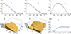Fig. 8 Distributions of angular distances in region C for all G. The blue points in the panels a, b, and c represent the data on ${\widehat{x}}_{ij},{\widehat{y}}_{ij},{\widehat{d}}_{ij}$ and the red curves are the result of a Monte-Carlo simulation. Panel f: ratio of data to the simulation from panel c. Panels d and e: 3D plots of distances xij, yij ; their unit is 1′′ . Panel e: region of small distances in higher resolution.

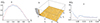Fig. 9 Distributions of angular distances in region C for G ≤ 15. The blue points in panel a represent the data on ${\widehat{d}}_{ij}$ and the red curve is the result of a Monte-Carlo simulation. Panel b: 3D plot of distances xij, yij, their unit is 1′′ . Panel c: ratio of data to simulation from panel a.

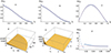Fig. 10 Distributions of angular distances in the region N&S for all G. The blue points in the panels a, b, and c represent the data on ${\widehat{x}}_{ij},{\widehat{y}}_{ij},{\widehat{d}}_{ij}$ and the red curves are result of Monte-Carlo simulation. Panel f: is the ratio of data to simulation from panel c. Panels d and e: 3D plots of distances xij , yij ; their unit  is 1′′ . Panel e: region of small distances in higher resolution.

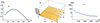Fig. 11 Distributions of angular distances in the region N&S for G ≤ 15. The blue points in panel a represent the data on ${\widehat{d}}_{ij}$ and the red curve is the result of a Monte-Carlo simulation. Panel b: 3D plot of distances xij , yij ; their unit is 1′′ . Panel c: ratio of data to simulation from panel a.

Fig. 12 3D plot of angular ternary distances xijk, yijk (unit is 1′′ ) in the region N&S for all G (a) and ratios of measured distribution of relative distances ${\widehat{d}}_{ijk}$ to the interpolation of corresponding Monte-Carlo distribution for all G (b) and G ≤ 18 mag (c).

3.2 Gravitational microlensing

The principle of the gravitational microlensing effect is explained in Schneider et al. (1992). For a small angular separation β between two stars, the light beams from the more distant one (S₂) and passing the gravitational field of the star on the way (S₁) can reach the observer by the two pathways, as illustrated in Fig. 13a. The angles seen by the observer are 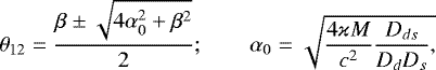$${\theta }_{12}=\frac{\beta \pm \sqrt{4{\alpha }_0^2+{\beta }^2}}{2};{\alpha }_0=\sqrt{\frac{4\varkappa M}{c^2}\frac{D_{ds}}{D_d{D}_s},}$$(47)

where ϰ is a gravitational constant, and M is the mass of the star S₁. For β =0 the Einstein ring with angular radius θ = α₀ is created. The relation in Eq. (47) implies $$\left|{\theta }_2\right|\le {\alpha }_0\le {\theta }_1.$$(48)

Therefore the necessary condition for observation of the splitting is that resolving power of the equipment is better than α₀ . For estimation of α₀, first of all the distance D_d is critical. For example D_d ≈ 10 − 10²l.y., D_s ≈ 2D and M ≈ M_S give roughly α₀ ≈ 20 mas. Such a small separation is probably beyond present Gaia resolution. In fact the minimum separation we have registered in any of the regions C, N, and S is 59 mas. At the same time, for observation of the effect it is important that angular separation β of the pair is close to α₀. For β < α₀, the sources S ₂ (θ₂), S₂(θ₁) become strongly magnified, so the source S₁ may not be resolved. On the other hand, brightness of S₂(θ₂) falls rapidly for β > α₀ (Schneider et al. 1992).

There can be the following signature of the gravitational microlensing effect. The light sources S ₂ (θ₂), S₁, S₂(θ₁) as seen by the observer, should have a small separation d_ijk (or ${\widehat{d}}_{ijk}$) and should be aligned, or make a narrow triangle within the errors of measurement (Fig. 13b,c). Therefore, as a measure of the alignment we define the parameter κ: 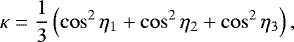$$\kappa =\frac{1}{3}\left({\cos }^2{\eta }_1+{\cos }^2{\eta }_2+{\cos }^2{\eta }_3\right),$$(49)

where η_i are angles in the observed triangle. For κ = 1 there is maximum alignment (e.g., η₁, η₂, η₃ = 0, 0, π) and for η₁ = η₂ = η₃ = π∕3 we have a minimum of κ = 1∕4. In the upper panels of Fig. 14 we have shown results of the uniform MC simulation. In the lower part we have shown its comparison with the data from the region N&S (we note the rescaled variable $d_{ijk}=2\rho {\widehat{d}}_{ijk}$). It is important that the shape of (normalized) MC distribution $P({\widehat{d}}_{ijk},$ κ) does not depend on the multiplicity of events M ≥ 3. The reasons are the same as for distributions $P({\widehat{d}}_{ijk})$ in Sect. 2.3. The same holds for the distribution P(κ) and the dependence $\langle \kappa \rangle$ on d_ijk. One can observe a perfect agreement with the data for d_ijk ≳ 5′′. On contrary, for the smaller distances among the three sources there is a clear excess of the alignment. Could there be a connection between this effect and the gravitational microlensing – image splitting? Or, more probably, is the excess only another form of the distortion of measurement at small separations?

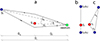Fig. 13 Geometry of gravitational microlensing effect (a). Alignment of three sources seen by observer: perfect (b) and partial (c).

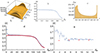Fig. 14 MC simulation of distribution $P({\widehat{d}}_{ijk},\kappa )$ (a), alignment function $\langle \kappa \rangle$ (b), and integrated distribution P(κ) (c). Panel d: comparison of $\langle \kappa \rangle$ from the data region N&S (blue) with the MC simulation (red). Panel e: same as panel d but in higher resolution.

4 Summary and conclusion

We have proposed a general statistical method for the analysis of finite 2D patterns. Each pattern (event) consists of the stars located inside the circle of a given radius. We have demonstrated that the method can identify tiny deviations from uniform distributions; for example, a tendency to display clustering or anti-clustering.

The method has been applied to the analysis of astrometric data obtained by the Gaia mission. In parallel with the data, we have generated a large set of random uniform events using the MC code. In thepresent study we have focused on the events of a small radius and correspondingly small multiplicity (M ≲ 10). We have shown the functions Θ_n(ρ, M) representingdeviations from random uniform distribution are a useful tool for analysis. An equally important tool is the set of functions $P\left(\widehat{\xi }\right)-$ distributions of the parameters characterizing mutual positions and distances among the stars (doublets and triplets). The results of our analysis are based on the comparison of these functions from both the data and the MC simulation. The main results are as follows.

• 1)

  In the dense region (C) we observe a 2D representation of reduced resolution power of two close sources (d_ij ≲ 4′′). Resolution improves for brighter pairs (G < 15).

• 2)

  In the sparse region (N&S) we observe an evident excess of the close pairs (d_ij ≲ 9′′). The effect is very pronounced for the bright pairs (G < 15). A similar effect is observed for the triplets. We interpret these excesses as the presence of binary and ternary star systems.

• 3)

  Apart from these effects we do not observe any violation of the uniformity on the scale of our events, which is defined by their radius ρ = 18′′(72′′) for the dense (sparse) region.

Special attention has been paid to the discussion on the possibility of detection of the gravitational microlensing and image splitting effect. Our present conclusion is that the statistical method suggested here can be a useful tool for detection of this effect. With the use of the alignment function $\langle \kappa \rangle$ we have observed the excess of the three-source alignment at separation <5′′, which could accompany the gravitational image splitting. At the same time we are aware of some incompleteness in the Gaia survey reported by the Gaia team for this scale. We believe it will be possible to obtain more consistent results from the next Gaia data release (DR2).

Acknowledgements

This work has made use of data from the European Space Agency (ESA) mission Gaia (https://www.cosmos.esa.int/gaia), processed by the Gaia Data Processing and Analysis Consortium (DPAC; https://www.cosmos.esa.int/web/gaia/dpac/consortium). Funding for the DPAC has been provided by national institutions, in particular the institutions participating in the Gaia Multilateral Agreement. The work was supported by the project LTT17018 of the MEYS (Czech Republic). Further, we are grateful to J. Grygar for deep interest and many valuable comments, J. Vondrak for critical reading of the manuscript and important comments, D. Heyrovsky and A. F. Zakharov for illuminating discussions on the gravitational microlensing effect and O. Teryaev for very useful discussions and inspiring comments.

References

All Tables

All Figures

	Fig. 1 Patterns of the stars inside the grid of circles (a). Position n0 of the event defines its local reference frame (b).
In the text

Fig. 2 Examples of deviations from uniform angular distribution defined by Eq. (16). The red curves are their representation in polar coordinates (P(ψ), ψ) as indicated in the lower left panel. The panels from left to right correspond to n = 1, 2, 3, 4. The upper (lower) panels correspond to the negative (positive) sign of vn = ∓1∕6. The black dot-dashed circles correspond to uniform distribution P(ψ) = 1.

In the text

	Fig. 3 Examples of the events generated by different algorithms: uniform distribution (a), clustering λ = 1∕3 (b), and anti-clustering λ = 1∕20 (c).
In the text

	Fig. 4 The functions Θn(M), n = 1, 2, 3 for Monte-Carlo events in the scenario of uniform distribution (upper panels). The remaining panels show clustering λ = 1∕3 (middle panels) and anti-clustering scenarios λ = 1∕20 (lower panels). Each multiplicity bin is generated by NM = 6000 events. The red lines correspond to the expected dependence for uniform distribution, Θ n (M) = 1 (Eq. (34)).
In the text

	Fig. 5 Distributions of angular distances $P({\widehat{x}}_{\alpha })$ of uniformly generated stars (points) fitted by the red curves (Eq. (45)). Corresponding distribution $P({\widehat{x}}_{\alpha },{\widehat{y}}_{\alpha })$ is on the right. Variables in panels are defined by relations (41)–(44). The Monte-Carlo statistics is represented by 2.5 × 106 events of multiplicity M = 5.
In the text

	Fig. 6 Analyzed regions in the Gaia catalog, where ρ is angular radius of the events, M is their multiplicity and Ne is the number of events. Analysis is done only for events 2 ≤ M ≤ 15.
In the text

	Fig. 7 The functions Θn(M), n = 1, 2, 3 for events in the area C (upper panels) and N&S (lower panels). The green line is a linear fit of data taken in panel Θ 2.
In the text

Fig. 8 Distributions of angular distances in region C for all G. The blue points in the panels a, b, and c represent the data on ${\widehat{x}}_{ij},{\widehat{y}}_{ij},{\widehat{d}}_{ij}$ and the red curves are the result of a Monte-Carlo simulation. Panel f: ratio of data to the simulation from panel c. Panels d and e: 3D plots of distances xij, yij ; their unit is 1′′ . Panel e: region of small distances in higher resolution.

In the text

	Fig. 9 Distributions of angular distances in region C for G ≤ 15. The blue points in panel a represent the data on ${\widehat{d}}_{ij}$ and the red curve is the result of a Monte-Carlo simulation. Panel b: 3D plot of distances xij, yij, their unit is 1′′ . Panel c: ratio of data to simulation from panel a.
In the text

Fig. 10 Distributions of angular distances in the region N&S for all G. The blue points in the panels a, b, and c represent the data on ${\widehat{x}}_{ij},{\widehat{y}}_{ij},{\widehat{d}}_{ij}$ and the red curves are result of Monte-Carlo simulation. Panel f: is the ratio of data to simulation from panel c. Panels d and e: 3D plots of distances xij , yij ; their unit  is 1′′ . Panel e: region of small distances in higher resolution.

In the text

	Fig. 11 Distributions of angular distances in the region N&S for G ≤ 15. The blue points in panel a represent the data on ${\widehat{d}}_{ij}$ and the red curve is the result of a Monte-Carlo simulation. Panel b: 3D plot of distances xij , yij ; their unit is 1′′ . Panel c: ratio of data to simulation from panel a.
In the text

	Fig. 12 3D plot of angular ternary distances xijk, yijk (unit is 1′′ ) in the region N&S for all G (a) and ratios of measured distribution of relative distances ${\widehat{d}}_{ijk}$ to the interpolation of corresponding Monte-Carlo distribution for all G (b) and G ≤ 18 mag (c).
In the text

	Fig. 13 Geometry of gravitational microlensing effect (a). Alignment of three sources seen by observer: perfect (b) and partial (c).
In the text

	Fig. 14 MC simulation of distribution $P({\widehat{d}}_{ijk},\kappa )$ (a), alignment function $\langle \kappa \rangle$ (b), and integrated distribution P(κ) (c). Panel d: comparison of $\langle \kappa \rangle$ from the data region N&S (blue) with the MC simulation (red). Panel e: same as panel d but in higher resolution.
In the text

References

- Adam, J., et al. (ALICE Collaboration) 2016, Phys. Rev. Lett., 116, 132302 [CrossRef] [PubMed] [Google Scholar]
- Arenou F., Luri X., Babusiaux C., et al. 2017, A&A, 599, A50 [NASA ADS] [CrossRef] [EDP Sciences] [Google Scholar]
- Gaia Collaboration (Brown, A. G. A., et al.) 2016a, A&A, 595, A2 [NASA ADS] [CrossRef] [EDP Sciences] [Google Scholar]
- Gaia Collaboration (Prusti, T., et al.) 2016b, A&A, 595, A1 [NASA ADS] [CrossRef] [EDP Sciences] [Google Scholar]
- Poskanzer, A. M., & Voloshin, S. A. 1998, Phys. Rev. C, 58, 1671 [CrossRef] [Google Scholar]
- Rustamov, A., & Rustamov, J. N. 2016, Arxiv e-prints [arXiv: 1602.01812] [Google Scholar]
- Schneider, P., Ehlers, J., & Falco, E.E. 1992, Gravitational Lenses (Berlin: Springer Verlag), XIV, 560 [Google Scholar]
- Voloshin, S., & Zhang, Y. 1996, Z. Phys. C, 70, 665 [CrossRef] [Google Scholar]