| Issue |
A&A
Volume 614, June 2018
|
|
|---|---|---|
| Article Number | A74 | |
| Number of page(s) | 11 | |
| Section | Extragalactic astronomy | |
| DOI | https://doi.org/10.1051/0004-6361/201731869 | |
| Published online | 15 June 2018 | |
Core-shifts and proper-motion constraints in the S5 polar cap sample at the 15 and 43 GHz bands
1
Departament d’Astronomia i Astrofísica, Universitat de València,
C/Dr. Moliner 50,
46100
Burjassot, Spain
e-mail: This email address is being protected from spambots. You need JavaScript enabled to view it.
2
Department of Earth, Space and Environment, Chalmers University of Technology, Onsala Space Observatory,
43992
Onsala, Sweden
3
Observatori Astronòmic, Universitat de València, Parc Científic,
C. Catedrático José Beltrán 2,
46980
Paterna,
València, Spain
Received:
31
August
2017
Accepted:
16
February
2018
Abstract
We have studied a complete radio sample of active galactic nuclei with the very-long-baseline-interferometry (VLBI) technique and for the first time successfully obtained high-precision phase-delay astrometry at Q band (43 GHz) from observations acquired in 2010. We have compared our astrometric results with those obtained with the same technique at U band (15 GHz) from data collected in 2000. The differences in source separations among all the source pairs observed in common at the two epochs are compatible at the 1σ level between U and Q bands. With the benefit of quasi-simultaneous U and Q band observations in 2010, we have studied chromatic effects (core-shift) at the radio source cores with three different methods. The magnitudes of the core-shifts are of the same order (about 0.1 mas) for all methods. However, some discrepancies arise in the orientation of the core-shifts determined through the different methods. In some cases these discrepancies are due to insufficient signal for the method used. In others, the discrepancies reflect assumptions of the methods and could be explained by curvatures in the jets and departures from conical jets.
Key words: astrometry / techniques: interferometric / quasars: general / BL Lacertae objects: general / radio continuum: general / techniques: high angular resolution
© ESO 2018
1 Introduction
Supermassive black holes are thought to be the engines of active galactic nuclei (AGNs) and enormous relativistic jets may be powered by them. These jets show very strong and compact radio emission. The “core” of the jet is the most compact feature, commonly related to the surface at which the optical depth becomes τ ≈ 1. Due to opacity and synchrotron self-absorption (SSA) effects, the position of the core, often the position of the peak intensity (i.e., the τ ≈ 1 surface) depends on the observing frequency (e.g., Blandford & Königl 1979; Königl 1981; Lobanov 1998). Since the re-absorption of synchrotron radiation is more efficient at low frequencies, the peak will appear further downstream along the jet axis as the observing frequency decreases.
The first detection of this “core-shift” effect was found by Marcaide & Shapiro (1983), and has since played a crucial role, not only in high-precision astrometry studies (e.g., Porcas 2009; Charlot 2010; Rioja et al. 2015), but also in the understanding of the jet structures (e.g., gradients of magnetic fields, pressure, and density) near the central engine of AGNs (e.g., Lobanov 1998; Martí-Vidal et al. 2011; Fromm et al. 2013). Detailed studies of the core-shifts in the astrometric catalogues may thus provide essential information for different aspects of astronomy; from geodesy and astrometry (i.e., to determine and remove the core-shift contribution in the alignment of the sources at different radio frequencies) to AGN astrophysics (understand how the jets form and propagate). In addition to this, a precise knowledge of the core-shift of distant quasars is essential to properly link radio and optical astronomical inertial reference frames. Systematic offsets in the positions of the reference sources between radio and optical observations have already been reported (Kovalev et al. 2017; Petrov & Kovalev 2017) due to the aforementioned core-shift effect and/or to non-negligible optical contributions from jet features.
Several methods for measuring the core-shift have been proposed. Rioja & Dodson (2011) presented a source-frequency phase-referencing (SFPR) method that makes it possible to perform an intra-source dual-frequency calibration, which is particularly convenient at high frequencies. Croke & Gabuzda (2008) developed a program to determine the shift between two VLBI images based on a cross-correlation analysis of the images, making use of all optically thin regions in the source structure. Kovalev et al. (2008) measured the core-shift of 29 compact extragalactic radio sources by model-fitting the source structure with two-dimensional Gaussian components, and referencing the core position to optically thin jet features whose positions are expected to be frequency-independent.
The study of core-shifts (as well as absolute proper motions) in a complete radio sample was indeed the main science driver of a large VLBI astrometry programme of observations of the complete S5 polar cap sample (13 radio-loud AGNs around the North Celestial Pole, e.g., Eckart et al. 1986) in phase-referencing mode, covering a frequency range from 1.4 to 43 GHz. Partial results for some of those observations (study of the source structures) have already been reported at the different bands (Ros et al. 2001; Pérez-Torres et al. 2004), as well as astrometry results for subsets of the sample (Ros et al. 1999; Guirado et al. 2000; Pérez-Torres et al. 2000; Guirado et al. 2004; Jimenez-Monferrer et al. 2007). The first global astrometry analysis (where the relative positions among source pairs at 15 GHz could be determined with unprecedented accuracy) was published in Martí-Vidal et al. (2008). In 2010, for the first time in this astrometry project, we used the fast-frequency-switching (FFS, see e.g., Middelberg 2005) observing capabilities of the very-long-baseline-array (VLBA). The observations were carried out at U and Q bands quasi-simultaneously. This approach enables us to perform one single (i.e., global and self-consistent) fit of the source positions at both frequencies, and thus, to obtain the shift of the positions between the low and high frequencies (i.e., the core-shift). Results of the global astrometry at U band, together with core-shift estimates based on the SFPR technique, were reported in Martí-Vidal et al. (2016).
In this paper, we present the first global differential phase-delay astrometry at a frequency as high as 43.1 GHz, likely the limit of application of this technique with current instrumentation, due to the relatively short ambiguities of the phase delays compared to the atmospheric variability at timescales of the order of the slewing times of the antennas. The power of the phase-delay astrometry analysis relies on the possibility of a simultaneous fit of all the parameters that define both the geometric and the instrumental components of the interferometer, such as clock drifts, position of the antennas, and tropospheric/ionospheric delays, together with the source positions. All these parameters are optimized self-consistently in the analysis, as opposed to other non-parametric approaches (e.g., phase referencing), where the instrumental and atmospheric effects are not properly parameterized and optimally accounted for for all sources, but rather estimated and interpolated from one calibrator to a target.
In addition to this global astrometry analysis, we study and compare three different methods to estimate the core-shift inseveral sources of this sample: 1) the global differenced phase-delay astrometry at 14.4 GHz (U band), directly compared to the global astrometry at 43.1 GHz (Q band); 2) a combined (i.e., simultaneous) global astrometry at the two bands; and 3) a slightly modified version of the SFPR technique, as previously reported for these observations in Martí-Vidal et al. (2016). As a complementary study, we also compare thecore-shift directions (for the subset of sources with successful detections) with the orientation of the core emission at the two frequencies, as a study of the jet geometry at (sub)-parsec scales.
In the following section, we describe the VLBA observations, the calibration strategy, and the analysis of the data. In Sect. 3 we describe the details of our astrometric analysis. In Sect. 4 we present the results of the global astrometry at Q band as well as the core-shifts obtained with the different methods. We summarize our results and conclusions in Sect. 5
2 Observations and data calibration
The observations analyzed here were already reported in Martí-Vidal et al. (2016). Therefore, we refer to that publication for all the details about the recording setup and the arrangement of the phase-referencing duty cycles. For convenience, we briefly summarize some of the details of those observations.
We used the fast frequency-switching (FFS) mode of the VLBA to observe at both U and Q bands (i.e., 14.4 GHz and 43.1 GHz, respectively), by inserting observations at the different bands in quasi-simultaneous scans. For the phase, delay, and phase-rate calibration, we applied the Global Fringe Fitting (GFF) algorithm (Alef & Porcas 1986) to all data at both bands. We only detected fringes at Q band for a subset of all sources observed (see Table 1). Our phase-delay analysis approach (see Sect. 4.3) requires detection of fringes at both bands in consecutive scans, and a sufficiently long integration time, for a robust estimate of the inter-frequency (core-shift) astrometry. Hence, we could only perform our core-shift analysis on a subset of the S5 Polar Cap Sample (right column in Table 1).
The data were calibrated using the AIPS1 program of NRAO, as described in Martí-Vidal et al. (2008). The phase contributions of the source structures were removed from the GFF gain solutions, and the phase (and group) delays were exported for their analysis with the University of Valencia Precision Astrometry Package (UVPAP) software (Martí-Vidal et al. 2008). The source pairs available to perform the global differenced astrometry at Q band are listed in Table 2. We notice that, even though we have good observations of sources 00 and 02, we could not compute their differential phase-delays due to the lack of detections of source 01 at Q band (observed in the same duty cycle).
Individual sources observed.
Source pairs observed at Q band sorted by increasing angular separations.
3 Astrometry analysis
3.1 Phase-delay connection
The phase connection at 43.1 GHz is especially difficult, since the delay corresponding to one 2π phase cycle is so short (only ~ 23 ps) that very small unmodeled atmospheric effects can add several 2π cycles to the phase-delays between two consecutive observations of the same source. A parameterized interferometer model (with station-based clock drifts described by third-order polynomials and atmospheric delays described by piece-wise linear functions) was fitted to the group delays, which provided a prediction of the phase delay rates good enough to ensure the proper connection of the phase-delays between consecutive scans of the same source. Since the average time separation between observations is ~ 180 s and the phase cycle at 43.1 GHz is ~ 23 ps, the residual rates have to be lower than (23 ps/180 s) 0.13 ps s−1 to ensure a good phase connection.
In Fig. 1, we plot the distribution of the residual delay rates of our observations. Residual delay rates with absolute values higher than 0.13 ps s−1 in the distribution, most of them corresponding to the longest baselines and the weakest sources, are not negligible. The model phase-delays were used to perform the connection of the observed phase-delays. Remaining 2π cycles were found by applying the automatic phase-connection algorithm described in Martí-Vidal et al. (2008). The few remaining (antenna-based) ambiguities, left after the connection process, were determined using the “smoothness criterion” described in the same publication.
This process of phase connection was first performed at U band (where the 2π phase ambiguities correspond to longer phase-delays of ~69 ps) and then the same parameterized model was used as the a priori model of the phase-delays at Q band.
 |
Fig. 1 Distribution of the residual delay rates for all the baselines, sources, and scans of our observations. The dashed lines at 0.13 ps s−1 illustrate that most of the values are good enough to ensure the phase-delay connection at 43.1 GHz (see text). |
3.2 Source-based clock offsets at Q band
The procedure used to estimate the source-based constant clock offsets (CCOs) at U band is described in Martí-Vidal et al. (2008). Basically, we apply an iterative process, where the CCOs are left as free parameters and we fix (one at a time) the closest CCO to a complete 2π phase-delay cycle. We iterate this procedure until all the source-based CCOs are fixed to complete 2π phase-delay cycles.
In Martí-Vidal et al. (2016), another automated procedure, where the CCOs are fixed in the frame of a Monte Carlo analysis for the estimate of the astrometric uncertainties is described. In that analysis, the source-based CCOs, together with the troposphericdelays, antenna positions, and even the dispersive ionospheric delays, are allowed to vary. From all these random deviations of the model parameters, we derive the posterior probability distributions of the source positions at U band (Martí-Vidal et al. 2016). In this analysis at 43.1 GHz we have followed the same procedure to derive the posterior probability distributions of the source positions at Q band.
The nodes of the piece-wise linear functions of the tropospheric delays are randomly perturbed following Gaussian distributions of 0.1 ns variance. We selected this uncertainty from the weather conditions of the experiment after we had evaluated the delay variations of the wet and dry components of the troposphere throughout the experiment. For the ionospheric delays, we apply random Gaussian perturbations in the total electron content (TEC), of variance 0.5 TECUs. Finally, for the antenna positions, we apply Gaussian perturbations of 1 cm variance (in each coordinate).
In Fig. 2, we show the distribution of CCO deviations from complete 2π phase-delay cycles at Q band, acquired from the whole set of Monte Carlo iterations. We notice that the CCO probability distribution has a clear peak near the integer number of 2π phase cycles, being minimum in the regionaround half 2π cycles. Sucha CCO distribution is expected from a successful phase connection, since the difference in phase-delays between antennas for each source shall be, by construction, an integer number of 2π cycles. The fact that we recover such values (from a completely free fit of the CCO values) is a good indicator that the time evolution of the delays for the different sources (which can cover several 2π cycles across the scans) are coherent from source to source, and during the whole experiment.
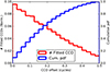 |
Fig. 2 Normalized distribution of constant clock offset deviations from complete 2π phase-delay cycles at 43.1 GHz. The red line represents the fitted values while the blue line represents the cumulative probability distribution function. We notice the peak near zero in the red line and, in the blue line, that half of the CCOs are within 0.15 cycles (~ 3.5 ps). |
4 Results
4.1 Differential phase-delay astrometry
The rms of the post-fit undifferenced delays range from 3.3 ps (baseline Kitt Peak−North Liberty observing source 08) to 36 ps (baseline Brewster−Kitt Peak observing source 19). For the differenced delays, the rms of the post-fit residuals range from 0.53 ps (Brewster−Pie Town observing the pair 19−20) to 10 ps (Fort Davis−Hancock observing the pair 18−20).
In Fig. 3, we show the undifferenced and differenced phase-delays for two representative baselines: Kitt Peak to Pie Town (KP), which corresponds to the shortest baseline in our sample (~ 420 km); and Hancock to Mauna Kea (HM), which corresponds to the longest baseline in our sample (~ 7500 km). The residual delays of all observed source pairs are shown in this figure.
The uncertainties in all observables were scaled to the rms of the post-fit residuals, arranged for each baseline and source pair, to minimize the effect of bad data on the final astrometric results (as also done in Martí-Vidal et al. 2008 and Martí-Vidal et al. 2016).
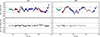 |
Fig. 3 Post-fit residual phase-delays for baselines Kitt Peak–Pie Town (left) and Hancock–Mauna Kea (right) for all observed sources: undifferenced delays (top); differenced delays (bottom). The dashed lines correspond to the delays of a ± 2π phase ambiguity at 43.1 GHz. Each color represents one source in the sample. The lack of residual differenced phase-delays between 20–25 h for the baseline HM is due to low S/N data of source 20 (magenta) in that interval. |
4.2 Changes in source separation with time and frequency
From the global astrometric analysis, we can analyze changes in the source core positions between our observations, either over time (i.e., between years 2000 and 2010) or between frequencies (i.e., Q and U bands). In our analysis, when the source structures are removed from the astrometric observables, a fiducial point in the source image has to be taken as the fiducial phase center (i.e., as the reference point in the source structure). We choose the brightness peak in the images as this phase-center point. By doing so, we minimize, by construction, the source-structure contribution to the visibility phases. Thus, the reference points in the astrometry are the intensity peaks of the sources. However, if there were any shift of the intensity peak with respect to any stable source component on the sky (e.g., the true source core), such a shift would appear as a position offset in our UVPAP astrometry analysis, in such a way that the true stable component of the source would remain fixed in the same position of the astrometry-corrected source image, across the different epochs.
We call θ the angular separation between a given pair of sources. As in Martí-Vidal et al. (2016), we have used source 07 (0716 + 734) as the absolute reference source in the Q band astrometry, because it has shown a rather compact structure at all epochs and frequencies. Since we relate the position of the sources to the intensity peaks at each frequency, we can think of the angular separation as a function of time (proper motions) and frequency (core-shifts). Thus, we can write θ(t, ν). In Martí-Vidal et al. (2016) we determined the changes in the angular separation between epochs for the case of almost the same frequency (ν ~ 15 GHz, U band). If we denote epochs 2000 and 2010 with indexes 1 and 2, respectively, the change in angular separation of a pair of sources between the two epochs at U band,  , will be
 (1)
(1)
where  and
and  are the angular separations of the pair of sources (at U band) in years 2000 and 2010, respectively. Indeed, these
  are the values reported in Table 3 and represented in Fig. 6 in Martí-Vidal et al. (2016). Since we have determined the position of the sources at Q band, we can now calculate the change in the angular separation between epochs and frequencies, i.e.,
 (2)
(2)
where  is the angular separation between a pair of sources at Q band in 2010. In Fig. 4, we show the changes in angular separation between sources as a function of source separation for the U band (epochs) and Q band (frequencies and epochs) with respectto the U1 reference positions.
Combining Eqs. (1) and (2) we can also calculate:
 (3)
(3)
Since we use the same a priori positions of the sources to calculate  and
and  ,
,  contains information about the combined core-shift of the pair of sources (i.e., the difference of the core-shifts between thetwo sources). We summarize the results of Eqs. (2) and (3) in Table 3. In Fig. 5, we show the difference in angular separation between sources at different frequencies in the year 2010. We find that all variations are compatible with zero at 1σ. Furthermore, if we apply the core-shift position corrections determined in Martí-Vidal et al. (2016) by means of phase-transfer phase-referencing calibration, we conclude that all frequency-dependent changes in the angular separations between sources are also compatible with zero at 1σ.
The uncertainties in the source motions between epochs 2000 and 2010 were estimated using a Monte Carlo approach. We generated a set of 1000 different realizations of the fit, obtained by adding random tropospheric delays, ionospheric delays, and antenna-position shifts, as discussed in Sect. 3.2. From each Monte Carlo iteration, the motions of all pairs of sources between epochs 2000 and 2010 were computed. The uncertainties in the motions were then obtained from their standard deviation over all the Monte Carlo iterations. The contributions to the error budget related to other (non-atmospheric) effects, such as station clocks or UT1–UTC, are much smaller than those included in the Monte Carlo analysis, and were already taken into account in the estimate of the position uncertainties made by UVPAP, which are based on the post-fit covariance matrix. These uncertainties were added in quadrature to those from the Monte Carlo analysis.
Results for the source pairs at U and Q bands.
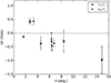 |
Fig. 4 Differences in source separations between years 2000 and 2010 among all the source pairs observed in common in the two epochs at the different frequencies. This is an updated version of Fig. 6 from Martí-Vidal et al. (2016). |
4.3 Inter-frequency differential phase-delay analysis
Once all the 2π ambiguities (and clock offsets) of the phase-delays are corrected at both bands, Q and U, all the data can be included into a single self-consistent fit (comprising data from both bands). The differences of delays between the bands for each source (we call them inter-frequency differential phase-delays (IFDPDs)) are sensitive to the change of source position with frequency (i.e., the core-shift). Given that the ionospheric effects were removed from the group (and phase) delay observables before the phase connection (using IONEX maps, as described in Martí-Vidal et al. 2008), at least to a first-order approximation, the remaining effects in the data are all non-dispersive (i.e., numerically the same for both bands). Therefore, we can use the same atmospheric model, clock drifts, and antenna positions to fit the delays at the two frequencies.
There is, though, a small instrumental effect left between the bands, which is related to the different optical paths followed by the signals at the different frequencies, from the antenna sub-reflectors to the VLBI backends. We account for this effect by including a new set of fittingparameters into the model, in the form of antenna-dependent constant clock offsets (common to all sources), for only Q band. If τU and τQ are the delays at U and Q band, respectively, for a given source at a given baseline and time, then
 (4)
(4)
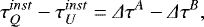
where τgeo is related to antenna positions and atmosphere (the same at both bands), τsou is the delay induced by source position (which encodes the core-shift) and τinst contains the instrumental effects (clock drifts and optical path into the system). The drift of the maser is the same at both bands, so that  –
– is only affected by the different (and constant) optical path of the signals between U and Q bands. This delay is modeled as
 (5)
(5)
where A and B are the antennas in the baseline and ΔτX is the extra path of the Q signal (with respect to U) at antenna X (i.e., the extra clock offsets added to the UVPAP model, for the IFDPD analysis). Using this set of extra parameters, the differences in phase-delays at the two frequencies can be used to determine the core shift, since Eq. (5) models the instrumental delay, so that only the term  –
–  remains unmodeled in Eq. (4.)
The IFDPD analysis is performed in a global fit, where all sources are fitted to the same geometrical and instrumental interferometer model. As was discussed in Martí-Vidal et al. (2008), the use of more than two sources in a global differential-astrometry fit increases the precision and robustness of the astrometry results, due to the extra redundancy in the observables (i.e., the same clock drifts and atmospheric model apply to all the differentsources and source pairs). Extending the global analysis to the IFDPD observables has thus clear advantages compared to the standard SFPR technique, where each target uses only gains interpolated from one calibrator.
We performed the IFDPD analysis, using a Monte Carlo approach, to determine the effects of atmosphere, clocks, and antenna positions on the estimated core-shifts. The atmospheric delay at each station was allowed to vary following Gaussian distributions with a variance of 0.1 ns (for the troposphere) and 0.5 TECU (for the ionosphere), which are realistic estimates of the uncertainty levels in the atmospheric models, as we previously discussed in Sect. 3.2. The antenna positions were left to vary following Gaussian distributions with a variance of 1 cm. On each iteration, the (antenna-dependent) CCOs were found for each antenna and source at Q band in an automatic way, as was also done in the global Q-band fit (see Sect. 3.2). In Fig. 6, we show the 2D histograms of the core-shifts for all sources with successful fringe detections at both bands, as estimated from the IFDPD analysis. The core-shift estimates obtained with the SFPR technique (reported in Martí-Vidal et al. 2016) are shown as red crosses for the sources with successful SFPR detections.
For sources 10, 11, and 18 the IFDPD core-shifts are almost degenerate (at sub-mas scales) among different directions on the sky. This degeneracy indicates strong coupling with the varying parameters in the Monte Carlo analysis (mainly, the atmosphere and its cross-talk with the CCOs at Q band). For source 20, the uncertainty derived from the Monte Carlo analysis is very large (of theorder of a milliarcsecond in the major axis of the 2D histogram distribution), which makes the result unusable. For sources 07, 00, 02, and 08 the IFDPD core-shifts have lower uncertainties, although we see a remarkable difference between the IFDPD and the SFPR core-shift estimates for source 07. At the moment of writing, we do not find any explanation for such a difference between the two methods. The SFPR result seems to agree better with the source morphology (Martí-Vidal et al. 2016).
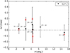 |
Fig. 5 Differences in source separations between U and Q bands in 2010. The red crosses correspond to the changes in angular separations estimated from the core-shift position corrections given in Martí-Vidal et al. (2016). |
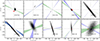 |
Fig. 6 In black, 2D histograms of the core-shifts in the S5 polar cap sample estimated from the IFDPD analysis (see Sect. 4.3). In red crosses, core-shifts estimated using the SFPR technique (Martí-Vidal et al. 2016). Blue (green) shaded areas indicate the orientations (within 1σ) of the main axis of the Gaussian intensity distributions fitted to the jet cores at U (Q) band (see Sect. 4.4). |
4.4 Visibility model-fitting of the core emission
As a complement to our global differenced phase-delay analysis, we have carried out a morphological study of the core regions at both bands. In principle, and as long as the core regions can be resolved at our VLBI resolutions, we would expect that the elongation of the jets in the core regions would be aligned to the direction of the core shifts. In addition to this, and according to the standard jet interaction model (e.g., Blandford & Königl 1979), the elongations of the core regions at both bands should have a similar orientation, as long as the jets are straight in these regions. Indeed, if the core emission at U and Q bands comes from the conical regions of the jets, the core sizes should be inversely proportional to the observing frequencies (e.g., Blandford & Königl 1979; Marscher 1980; Martí-Vidal et al. 2011).
Any deviation of the core morphology from these predictions, which are based on the standard jet model, may indicate either bent jet geometries or emission from non-conical (i.e., concave) jet regions, likely related to the Poynting-flux-dominated zone of the outflows close to the jet bases (e.g., Marscher 1980; Marscher et al. 2008; Martí-Vidal et al. 2013).
We have used the UVMULTIFIT program (Martí-Vidal et al. 2014), based on the CASA2 software by NRAO, to derive the sizes, morphologies, and orientations of the core regions of all sources detected in both bands. We model the morphology of the core emission in two steps. First, we fit the visibilities using one single elliptical Gaussian intensity distribution, centered at the intensity peak (the Gaussian position is left free in the fit, but witha constraint equal to the full width at half maximum (FWHM) of the restoring beam). Then, we CLEAN thepost-fit residual visibilities and define a second Gaussian intensity distribution, located now at the peak intensity of the residual image. This Gaussian is used to model any residual emission close to the core. The position of this second Gaussian is also left free, but with similar constraints to those of the first Gaussian. These two Gaussians are fitted simultaneously (to enable cross-talk between their structure parameters in the fit). This approach helps to minimize biases related to component blending at the core region, as long as the signal-to-noise ratio (S/N) of the visibilities is high enough (which is our case for all sources). We notice that this kind of analysis via Gaussian fitting is routine in VLBI analyses of AGN core-jet structures (e.g., the MOJAVE analysis procedure, Lister et al. 2009, 2013).
In Figs. 7 and 8, for example, we present some images that show the Gaussian fitting to the core+jet regions (left), as well as images of the post-fit residuals (right). In all cases, the unmodeled (i.e., residual) post-fit peak intensities are considerably lower than the pre-fit peak intensities. This indicates that most of the core emission can indeed be successfully modeled with an elliptical Gaussian intensity distribution. In Fig. 6, we show the orientations (within 1σ) of the main axis of the Gaussian intensity distributions fitted to the jet cores at both bands.
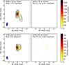 |
Fig. 7 Left: images of sources 08 (top) and 10 (bottom) at U band showing the core+jet emission fitted to Gaussian emission distributions (see text). The contours are spaced logarithmically in ten levels, running from two times the rms of the residuals to the image peak. Right: post-fit residuals of UVMULTIFIT after fitting Gaussian brightness distributions to the core+jet emission of each source. |
4.4.1 Fitting results
In Fig. 9, we show the orientations, ellipticities (i.e., minor-to-major axis ratios), and sizes of all the Gaussians fitted to the jet cores at both bands. Several conclusions can already be drawn from this comparison between the bands. On the one hand, the position angles of the major Gaussian axes are similar between the two bands for most sources (differences of a few sigmas are seen between the bands), with some outliers (sources 02, 07, 10, and 20). Hence, the jets seem to be rather straight for a large portion of the sample.
On the other hand, the axis ratio, which should be the same at both bands if the core emission originates in the conical jet region (since, in this region, the brightness distribution is self-similar at any frequency), shows remarkable systematics between the two bands. At the lowest frequency, the ratio is typically higher (i.e., the Gaussians are more elongated at the higher frequency). A natural explanation of this deviation from self-similarity is that there may be a contribution to the emission at Q band coming from the concave (i.e., Poynting-dominated) jet region, where there is a shallower dependence of the magnetic-field intensity and particle density with distance to the jet base (Marscher 1980), hence extending the core regions at the highest frequencies (Martí-Vidal et al. 2013). This interpretation is supported by the comparison of core sizes (Fig. 9, right), where the size of the minor Gaussian axis (i.e., the axis related to the width of the jet), when scaled by the frequency ratio from the observed U band size, is smaller than the observed Q band size. At the concave jet region, the jet width is not proportional to the distance from the jet base. Therefore, if the emission at Q band (or at least a fraction of it) comes from the concave jet region, the estimated jet width will be larger than the frequency-scaled size from the U band. Our results with visibility model-fitting thus seem to indicate that at least a fraction of the core emission at Q band is not originated in the conical jet region, and/or that the standard jet model may not apply to all sources in our sample at Q band. Of course, this will have an effect on the expected core shift, since it will be smaller in the concave jet region compared to that in the pure conicalmodel (e.g., Martí-Vidal et al. 2013).
4.4.2 Core-shifts vs. core-orientations
From the standard jet model, it is expected that the major axis of the Gaussian distributions fitted to the core (which would follow the local direction of the jet) will be in line with the direction of the core-shift. This statement holds as long as the jet remains straight in the region between the cores at both bands. We can test this by direct comparison of our core-shift estimates with the UVMULTIFIT results. Indeed, Rioja et al. (2015) find agreement between core-shift directions at several bands (from43 GHz up to 140 GHz), observed with the Korean VLBI Network (KVN) and the orientations of the jets in several AGNs. We notice, though, that the limited angular resolution of the KVN (beam larger than the core-jet regions) might introduce blending effects of the jet emission within the beam and partially mask the true core-shift in these sources. Instead, the VLBA angular resolution is adequate to resolve the core from the extended jets.
The two sources with highest S/N in the IFDPD core-shift estimates are 00 and 02 (see Sect. 4.3). In Fig. 10, we show a reconstruction of the jet core structure based on the Gaussians fitted with UVMULTIFIT. We show the full width at half maximum (FWHM) of the cores at both bands shifted one from the other using the IFDPD core-shift. For source 00, we see excellent agreement between the orientations of the Gaussians at both bands and the direction of the core-shift. This is indicative of a straight jet (we notice that source 00 falls on the 1:1 correlation in Fig. 9, left). Regarding source 02, the core-shift is almost aligned to the major axis of the core Gaussian at U band, although the core Gaussian at Q band shows a rotation of almost 90 degrees with respect to U band. This may be indicative of a strongly curved jet at pc scale from the central engine. Similar curved jet structures have indeed been reported for other AGNs (e.g., Savolainen et al. 2006; Molina et al. 2014).
A direct comparison between the SFPR core-shift direction and the orientation of the elliptical-Gaussian intensity distributions, fitted to the core emission at both bands, is shown in Fig. 11 (top). We notice that, for a correct comparison, an ambiguity of 180 degrees has to be applied to the position angles of the (axisymmetric) elliptical Gaussian distributions. We have done so by either adding or subtracting 180 degrees to the UVMULTIFIT estimates, so that the angles get as close as possible to the core-shift directions. For completeness, we show in Fig. 11 (bottom) the comparison between core position angles and IFDPD core-shift directions (only for those sources with clear, non-degenerate, detections). In both cases (SFPR and IFDPD), there is a hint of a weak correlation. For the SFPR, we find a correlation coefficient R2 of 0.59 and 0.56 for U and Q bands, respectively. Sources 19 and 07 are far from the correlation by about 50 degrees at both bands, whereas sources 08, 11, 10, 18 and 20 are about 20–40 degrees away.
The lack of a 1:1 correlation between the morphological jet direction (i.e., the position angle of the core Gaussian distributions) and the direction of the core shift indicates large departures of the sources from straight jets. Helicoidal jet shapes, coupled to opacity effects at the jet cores, could help explain both the different orientations of the cores at the different frequencies seen in some sources (Fig. 9, left), as well as the misorientation of the core-shift with respect to the core major axes (Fig. 11).
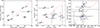 |
Fig. 9 Left: position angles of Gaussian intensity distributions fitted to the core emission at U band (horizontal axis) and Q band (vertical axis). Center, minor-to-major axis ratios of the same fitted Gaussian intensity distributions. Right: size of the minor Gaussian axis at U band (multiplied by the U/Q frequency ratio) vs. size of the minor Gaussian axis at Q band. |
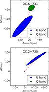 |
Fig. 10 Full width at half maximum (FWHM) of the Gaussian intensity distributions fitted to the cores of sources0016 + 731 (top) and 0212 + 735 (bottom). The U and Q distributions have been placed as indicated by the core-shifts estimated from our IFDPD analysis (red dashed line). We notice that the directions of the core-shifts almost coincide with the orientations of the main axis of the Gaussians at U band. |
 |
Fig. 11 Core-shift directions estimated using the SFPR (top) and the IFDPD (bottom) techniques vs. position angles of Gaussian intensity distributions fitted to the core emission at U (blue) and Q (green) bands. Only sources with successful (non-degenerate) core-shift detections are shown in the bottom figure. |
4.5 χ2 tests of jet resolution
The sizes of the Gaussian brightness distributions fitted with UVMULTIFIT are of the order of (or smaller than) the sizes of the synthesized VLBI beams. Therefore, eventual artifacts (related to source super-resolution) might be affecting the UVMULTIFIT results and/or non-unique elliptical Gaussians (i.e., different ellipticities and position angles) may fit the data with similarquality. If that was the case, the UVMULTIFIT estimates of jet orientations and sizes would not be robust.
We notice, though, that the possibility of achieving super-resolution in interferometric observations with high S/N is well studied (e.g., Martí-Vidal et al. 2012) and can indeed be routinely achieved with advanced deconvolution techniques, such as non-linear visibility model-fitting 3.
We have tested the robustness of the UVMULTIFIT results via tests of Likelihood Ratio (e.g., Wall & Jenkins 2012). The Likelihood Ratio gives us the probability of a model to be true against that of a null hypothesis, by comparing the probability ratio of the two models to the expected value of a χ2 distribution, whose number of parameters equals the difference in the number of fitting parameters of the two models being compared (i.e., the test model and the null-hypothesis model).
We performed two tests. On the one hand, the first test is a resolvability test, where the model of the null hypothesis is a point sourceand the test model is a circular Gaussian. In this case, the difference in degrees of freedom between models is one (i.e., the size of the Gaussian). On the other hand, the second test is an ellipticity test, where the model of the null hypothesis is a circular Gaussian and the test model is an elliptical Gaussian. In this case, the test model has two extra fitting parameters (i.e., axis ratio and position angle).
We notice that the Likelihood Ratio is sensitive to the absolute scale of the visibility uncertainties, which is not well defined (i.e., only the relative uncertainties can be estimated with precision during the calibration process of interferometry data). Indeed, the UVMULTIFIT program scales the visibility uncertainties after the fit, such that the post-fit reduced χ2 equals its expected value (i.e., unity). This assumes that the fitted model has been perfectly optimized to describe the data and could bias our hypothesis testing.
Therefore, in our Likelihood-Ratio tests, we have applied an alternative method to derive the correct absolute scale of the visibility uncertainties. We have assumed that the residual visibilities after a full CLEAN deconvolution (i.e., those for which the effects of the whole source structure have been completely removed) correspond to a reduced χ2 of unity. We measure the χ2 as a quantity proportional to the root-mean-square (rms) of the residual image (which is proportional to the rms in Fourier space, according tothe Parseval’s Theorem). This assumption allows us to derive a global scaling factor for the visibility uncertainties.
We have then used this scaling factor to derive the χ2 values for all the models fitted to the visibilities, by computing the rms of the images after the Fourier inversion of the post-fit residual visibilities. The resulting χ2 differences among models are given in Tables 4 and 5, together with the ratios between the χ2 improvements and those expected from the null hypothesis, with a p-value of 0.95. Hence, a ratio of one implies the acceptance of the test hypothesis with a likelihood of 0.95; ratios larger than one imply even higher probabilities for the acceptance of the test hypotheses. For cases where the χ2 of the null hypothesis is lower than that of the test hypothesis, we set a probability of 0 for the test hypothesis (and consider the test as failed). As can be seen in both Tables, the resolvability test is passed on all sources, whereas the ellipticity test passes on almost all cases at 43 GHz (it fails on 1749, and 1928) and at 15 GHz (it fails on 1039, 1150, and 1749).
Results of the Likelihood Ratio tests for the 43 GHz data.
5 Conclusions
We report on quasi-simultaneous VLBA observations of the S5 polar cap sample at U and Q bands, performed in December 2010 in phase-referencing mode, using the FFS capabilities of the VLBA, and compare them to earlier results at U band. We have performed a high-precision wide-angle astrometric analysis of a complete radio sample, and for the first time, we have globally connected the phase-delays at a frequency as high as 43.1 GHz. Since the delay corresponding to one 2π phase cycle at this frequency is so short (~23 ps), the Q band probably marks the observational limit for this astrometric technique, mainly due to the fast atmospheric variations and the long slewing time of the antennas between scans. A similar study at higher frequencies (e.g., 86 GHz with a phase cycle of ~ 12 ps), where the atmospheric conditions vary faster than at lower frequencies, might not be feasible with the current instrumentation.
Our successful global astrometric analysis at Q band enables us to study the changes in the source core positions between different epochs (year 2000 at U band and year 2010 at U∕Q bands) and/or between different frequencies (i.e., U and Q bands). From the inter-epoch analysis, we find that the differences in source separations among all the source pairs observed in common in the two epochs are compatible at the 1σ level between the U and Q bands. Besides, from an inter-frequency analysis in 2010, we find that the differences in source separations between U and Q bands are compatible at the 1σ level with those estimated from the core-shift position corrections given in Martí-Vidal et al. (2016) by means of the SFPR technique.
We have performed an IFDPD analysis to study the core-shift effect between the U and Q bands in a way that is independent from the SFPR technique. For sources 10, 11, and 18 the IFDPD core-shifts are almost degenerate (at sub-mas scales) across different directions on the sky, perhaps due to strong coupling between the parameters associated with the atmosphere (mainly residual ionosphere) and the CCOs at Q band in the Monte Carlo analysis. This issue might be leading to unreliable estimates of the core-shift directions for these sources. For sources 00, 02, 07, and 17 the uncertainties in the IFDPD core-shift directions are lower. The core-shift estimates of those sources are more accurate and less affected by atmospheric/CCO effects. The absolute values of the core-shifts determined with all methods presented in this paper are of the same order as those predicted by the statistical study of Kovalev et al. (2008) using a simplified SSA jet model (e.g., Lobanov 1998), if extrapolated to the whole S5 polar cap sample at U and Q bands.
We have fitted the core emission at U and Q bands to Gaussian intensity distributions. We find that the position angles of the major Gaussian axes are similar between the two bands for most of the sources except for some exceptions (sources 02, 07, 10, and 20). This result indicates that a considerable fraction of the total sample shows rather straight jets. Besides, we compared the core-shift directions to the core orientations at both bands and found that there is good agreement between the core orientations at U band and the core-shifts for the sources with the most accurate core-shift estimates (sources 00, 02, 07 and 17). This is an expected result since the orientation of the Q band core has less of an effect on the core-shift orientation than on the orientation of the U band core.
On the other hand, from the analysis of the axis ratio of the core Gaussians at each frequency, we conclude that at least a fraction of the Q band emission is likely to come from the concave jet region, where the jet width is not proportional to the distance from the jet base.
We have presented three different methods to study the core-shift effect and we conclude that, even though they do not agree in the estimate of the core-shift directions in some cases, they are all compatible in the absolute value of the core-shifts. In some cases, the discrepant orientations are due to insufficient signal for the method used. In other cases, the discrepancies reflect assumptions of the methods and could be explained by curvatures in the jets and departures from conical jets.
Results of the Likelihood Ratio tests for the 15 GHz data.
Acknowledgements
We thank Irwin I. Shapiro for comprehensive comments and suggestions that helped us to improve the manuscript. FJA, JMM, and JCG were partially supported by the Spanish MINECO projects AYA2012-38491-C02-01 and AYA2015-63939-C2-2-P and the Generalitat Valenciana projects PROMETEO/2009/104 and PROMETEOII/2014/057. IMV thanks the Alexander von Humboldt Foundation for his post-doctoral fellowship in years 2009−2011 (which covered a part of the research work reported here). The National Radio Astronomy Observatory is a facility of the National Science Foundation operated under cooperative agreement by Associated Universities, Inc.
References
- Alef, W., & Porcas, R. W. 1986, A&A, 168, 365 [NASA ADS] [Google Scholar]
- Bietenholz, M. F., Bartel, N., & Rupen, M. P. 2004, ApJ, 615, 173 [NASA ADS] [CrossRef] [Google Scholar]
- Blandford, R. D., & Königl, A. 1979, ApJ, 232, 34 [NASA ADS] [CrossRef] [Google Scholar]
- Charlot, P., Boboltz, D. A., Fey, A. L., et al. 2010, AJ, 139, 1713 [NASA ADS] [CrossRef] [Google Scholar]
- Croke, S. M., & Gabuzda, D. C. 2008, MNRAS, 386, 619 [NASA ADS] [CrossRef] [Google Scholar]
- Eckart, A., Witzel, A., Biermann, P., et al. 1986 A&A, 168, 17 [NASA ADS] [Google Scholar]
- Fromm, C. M., Ros, E., Perucho, M., et al. 2013, A&A, 557, A105 [NASA ADS] [CrossRef] [EDP Sciences] [Google Scholar]
- Guirado, J. C., Marcaide, J. M., Pérez-Torres, M. A., & Ros, E. 2000, A&A, 353, L37 [NASA ADS] [Google Scholar]
- Guirado, J. C., Marcaide, J. M., Ros, E., Pérez-Torres, M. A., & Martí-Vidal, I. 2004, Proc. of the 7th European VLBI Network Symp. (Observatorio Astrono Nacional of Spain), 327 [Google Scholar]
- Jimenez-Monferrer, S., Marcaide, J. M., Guirado, J. C., & Martí-Vidal, I. 2007, Proc. Sci., 103 [Google Scholar]
- Königl, A. 1981, ApJ, 243, 700 [NASA ADS] [CrossRef] [Google Scholar]
- Kovalev, Y. Y., Lobanov, A. P., Pushkarev, A. B., & Zensus, J. A. 2008, A&A, 483, 759 [NASA ADS] [CrossRef] [EDP Sciences] [Google Scholar]
- Kovalev, Y. Y., Petrov, L., & Plavin, V. 2017, A&A, 598, L1 [NASA ADS] [CrossRef] [EDP Sciences] [Google Scholar]
- Lister, M. L., Cohen, M. H., Homan, D. C., et al. 2009, AJ, 138, 1874 [NASA ADS] [CrossRef] [Google Scholar]
- Lister, M. L., Aller, M. F., Aller, H. D., et al. 2013, AJ, 146, 120 [NASA ADS] [CrossRef] [Google Scholar]
- Lobanov, A. P. 1998, A&A, 330, 79 [NASA ADS] [Google Scholar]
- Marcaide, J. M., & Shapiro, I. I. 1983, AJ, 88, 1133 [NASA ADS] [CrossRef] [Google Scholar]
- Marscher, A. P. 1980, ApJ, 235, 386 [NASA ADS] [CrossRef] [Google Scholar]
- Marscher, A. P., Jorstad, S. G., D’Arcangelo, F. D., et al. 2008, Nature, 452, 966 [NASA ADS] [CrossRef] [PubMed] [Google Scholar]
- Martí-Vidal, I., Marcaide J. M., Guirado J. C., Pérez-Torres, M. A., & Ros, E. 2008, A&A, 478, 267 [NASA ADS] [CrossRef] [EDP Sciences] [Google Scholar]
- Martí-Vidal, I., Marcaide, J. M., Alberdi, A., et al. 2011, A&A, 533, A111 [NASA ADS] [CrossRef] [EDP Sciences] [Google Scholar]
- Martí-Vidal, I., Pérez-Torres, M. A., & Lobanov, A. P. 2012, A&A, 541, A135 [NASA ADS] [CrossRef] [EDP Sciences] [Google Scholar]
- Martí-Vidal, I., Muller, S., Combes, F., et al. 2013, A&A, 558, A12 [NASA ADS] [CrossRef] [EDP Sciences] [Google Scholar]
- Martí-Vidal, I., Vlemmings, W. H. T., Muller, S., & Casey, S. 2014, A&A, 563, A136 [NASA ADS] [CrossRef] [EDP Sciences] [Google Scholar]
- Martí-Vidal, I., Abellán, F. J., Marcaide, J. M., et al. 2016, A&A, 596, A27 [NASA ADS] [CrossRef] [EDP Sciences] [Google Scholar]
- Middelberg, E., Roy, A. L., Walker, R. C., & Falcke, H. 2005, A&A, 433, 897 [NASA ADS] [CrossRef] [EDP Sciences] [Google Scholar]
- Molina, S. N., Agudo, I., Gomez, J. L., et al. 2014, A&A, 566, A26 [NASA ADS] [CrossRef] [EDP Sciences] [Google Scholar]
- Pérez-Torres, M. A., Marcaide, J. M., Guirado, J. C., et al. 2000, A&A, 360, 161 [NASA ADS] [Google Scholar]
- Pérez-Torres,M. A., Marcaide, J. M., Guirado, J. C., & Ros, E. 2004, A&A, 428, 847 [NASA ADS] [CrossRef] [EDP Sciences] [Google Scholar]
- Petrov, L., & Kovalev, Y. Y. 2017, MNRAS, 467, L71 [NASA ADS] [Google Scholar]
- Porcas, R. W. 2009, A&A, 505, 1 [Google Scholar]
- Rioja, M., & Dodson, R., 2011, AJ, 141, 114 [NASA ADS] [CrossRef] [Google Scholar]
- Rioja, M. J., Dodson, R., Jung, T., & Sohn, B. W. 2015, AJ, 150, 202 [NASA ADS] [CrossRef] [Google Scholar]
- Ros, E., Marcaide, J. M., Guirado, J. C., et al. 1999, A&A, 348, 381 [NASA ADS] [Google Scholar]
- Ros, E., Marcaide, J. M., Guirado, J. C., & Pérez-Torres, M. A. 2001, A&A, 376, 1090 [NASA ADS] [CrossRef] [EDP Sciences] [Google Scholar]
- Savolainen, T., Wiik, K., Valtaoja, E., et al. 2006, ApJ, 647, 172 [NASA ADS] [CrossRef] [Google Scholar]
- Wall, J. V., & Jenkins, C. R. 2012, Practical Statistics for Astronomers, (Cambridge, UK: Cambridge University Press) [CrossRef] [Google Scholar]
See, e.g., Martí-Vidal et al. (2011), where the jet of the AGN in M 81 was successfully modeled with an elliptical Gaussian, in a very similar way to the modeling performed here.
All Tables
All Figures
|
Fig. 1 Distribution of the residual delay rates for all the baselines, sources, and scans of our observations. The dashed lines at 0.13 ps s−1 illustrate that most of the values are good enough to ensure the phase-delay connection at 43.1 GHz (see text). |
| In the text | |
|
Fig. 2 Normalized distribution of constant clock offset deviations from complete 2π phase-delay cycles at 43.1 GHz. The red line represents the fitted values while the blue line represents the cumulative probability distribution function. We notice the peak near zero in the red line and, in the blue line, that half of the CCOs are within 0.15 cycles (~ 3.5 ps). |
| In the text | |
|
Fig. 3 Post-fit residual phase-delays for baselines Kitt Peak–Pie Town (left) and Hancock–Mauna Kea (right) for all observed sources: undifferenced delays (top); differenced delays (bottom). The dashed lines correspond to the delays of a ± 2π phase ambiguity at 43.1 GHz. Each color represents one source in the sample. The lack of residual differenced phase-delays between 20–25 h for the baseline HM is due to low S/N data of source 20 (magenta) in that interval. |
| In the text | |
|
Fig. 4 Differences in source separations between years 2000 and 2010 among all the source pairs observed in common in the two epochs at the different frequencies. This is an updated version of Fig. 6 from Martí-Vidal et al. (2016). |
| In the text | |
|
Fig. 5 Differences in source separations between U and Q bands in 2010. The red crosses correspond to the changes in angular separations estimated from the core-shift position corrections given in Martí-Vidal et al. (2016). |
| In the text | |
|
Fig. 6 In black, 2D histograms of the core-shifts in the S5 polar cap sample estimated from the IFDPD analysis (see Sect. 4.3). In red crosses, core-shifts estimated using the SFPR technique (Martí-Vidal et al. 2016). Blue (green) shaded areas indicate the orientations (within 1σ) of the main axis of the Gaussian intensity distributions fitted to the jet cores at U (Q) band (see Sect. 4.4). |
| In the text | |
|
Fig. 7 Left: images of sources 08 (top) and 10 (bottom) at U band showing the core+jet emission fitted to Gaussian emission distributions (see text). The contours are spaced logarithmically in ten levels, running from two times the rms of the residuals to the image peak. Right: post-fit residuals of UVMULTIFIT after fitting Gaussian brightness distributions to the core+jet emission of each source. |
| In the text | |
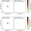 |
Fig. 8 As in Fig. 7, but at Q band. |
| In the text | |
|
Fig. 9 Left: position angles of Gaussian intensity distributions fitted to the core emission at U band (horizontal axis) and Q band (vertical axis). Center, minor-to-major axis ratios of the same fitted Gaussian intensity distributions. Right: size of the minor Gaussian axis at U band (multiplied by the U/Q frequency ratio) vs. size of the minor Gaussian axis at Q band. |
| In the text | |
|
Fig. 10 Full width at half maximum (FWHM) of the Gaussian intensity distributions fitted to the cores of sources0016 + 731 (top) and 0212 + 735 (bottom). The U and Q distributions have been placed as indicated by the core-shifts estimated from our IFDPD analysis (red dashed line). We notice that the directions of the core-shifts almost coincide with the orientations of the main axis of the Gaussians at U band. |
| In the text | |
|
Fig. 11 Core-shift directions estimated using the SFPR (top) and the IFDPD (bottom) techniques vs. position angles of Gaussian intensity distributions fitted to the core emission at U (blue) and Q (green) bands. Only sources with successful (non-degenerate) core-shift detections are shown in the bottom figure. |
| In the text | |
Current usage metrics show cumulative count of Article Views (full-text article views including HTML views, PDF and ePub downloads, according to the available data) and Abstracts Views on Vision4Press platform.
Data correspond to usage on the plateform after 2015. The current usage metrics is available 48-96 hours after online publication and is updated daily on week days.
Initial download of the metrics may take a while.