| Issue |
A&A
Volume 613, May 2018
|
|
|---|---|---|
| Article Number | A15 | |
| Number of page(s) | 31 | |
| Section | Cosmology (including clusters of galaxies) | |
| DOI | https://doi.org/10.1051/0004-6361/201732248 | |
| Published online | 23 May 2018 | |
Scale dependence of galaxy biasing investigated by weak gravitational lensing: An assessment using semi-analytic galaxies and simulated lensing data
1
Argelander-Institut für Astronomie, Universität Bonn,
Auf dem Hügel 71,
53121
Bonn, Germany
e-mail: This email address is being protected from spambots. You need JavaScript enabled to view it.
2
Faculty of Physics, Ludwig-Maximilians University,
Scheinerstr. 1,
81679
München,
Germany
3
Excellence Cluster Universe,
Boltzmannstr. 2,
85748
Garching, Germany
Received:
7
November
2017
Accepted:
12
December
2017
Abstract
Galaxies are biased tracers of the matter density on cosmological scales. For future tests of galaxy models, we refine and assess a method to measure galaxy biasing as a function of physical scale k with weak gravitational lensing. This method enables us to reconstruct the galaxy bias factor b(k) as well as the galaxy-matter correlation r(k) on spatial scales between 0.01 h Mpc−1 ≲ k ≲ 10 h Mpc−1 for redshift-binned lens galaxies below redshift z ≲ 0.6. In the refinement, we account for an intrinsic alignment of source ellipticities, and we correct for the magnification bias of the lens galaxies, relevant for the galaxy-galaxy lensing signal, to improve the accuracy of the reconstructed r(k). For simulated data, the reconstructions achieve an accuracy of 3–7% (68% confidence level) over the above k-range for a survey area and a typical depth of contemporary ground-based surveys. Realistically the accuracy is, however, probably reduced to about 10–15%, mainly by systematic uncertainties in the assumed intrinsic source alignment, the fiducial cosmology, and the redshift distributions of lens and source galaxies (in that order). Furthermore, our reconstruction technique employs physical templates for b(k) and r(k) that elucidate the impact of central galaxies and the halo-occupation statistics of satellite galaxies on the scale-dependence of galaxy bias, which we discuss in the paper. In a first demonstration, we apply this method to previous measurements in the Garching-Bonn Deep Survey and give a physical interpretation of the lens population.
Key words: gravitational lensing: weak / large-scale structure of Universe / cosmology: observations / galaxies: statistics
© ESO 2018
1 Introduction
The standard paradigm of cosmology describes the large-scale distribution of matter and galaxies in an expanding Universe (Dodelson 2003, and references therein). Strongly supported by observations, this model assumes a statistically homogeneous and isotropic Universe with cold dark matter (CDM) as the dominating form of matter. Matter in total has the mean density Ωm ≈ 0.3 of which ordinary baryonic matter is just Ωb ≈ 0.05; as usual densities are in units of the critical density (or its energy equivalent). The largest fraction ΩΛ ≈ 0.7 in the cosmological energy density is given by a cosmological constant Λ or so-called dark energy, resulting in a flat or approximately flat background geometry with curvature parameter K = 0 (Einstein 1917; Planck Collaboration XIII 2016, and references therein). The exact physical nature of dark matter is unknown but its presence is consistently inferred through visible tracers from galactic to cosmological scales at different epochs in the cosmic history (Bertone et al. 2005, for a review). In particular the coherent shear of distant galaxy images (background sources) by the tidal gravitational field of intervening matter gives direct evidence for the (projected) density field of dark matter (Clowe et al. 2004). The basic physics of galaxy formation inside dark-matter halos and the galaxy evolution seems to be identified and reasonably well matched by observations, although various processes, such as star formation and galaxy-gas feedback, are still not well understood or worked out in detail (Mo et al. 2010). Ultimately, the ability of the ΛCDM model to quantitatively describe the observed richness of galaxy properties from initial conditions will be a crucial validation test.
One galaxy property of importance is spatial distribution. Galaxies are known to be differently distributed than matter in general; they are so-called biased tracers of the matter density field (Kaiser 1984). The details of the biasing mechanism are related to galaxy physics (Springel et al. 2018, 2005; Weinberg et al. 2004; Somerville et al. 2001; Benson et al. 2000; Peacock & Smith 2000). An observed galaxy bias for different galaxy types and redshifts consequently provides input and tests for galaxy models. Additionally, the measurement of galaxy bias is practical for studies that rely on fiducial values for the biasing of a particular galaxy sample or on the observational support for a high galaxy-matter correlation on particular spatial scales (e.g. van Uitert et al. 2018; Hildebrandt et al. 2013; Simon 2013; Mehta et al. 2011; Reyes et al. 2010; Baldauf et al. 2010). In this context, we investigate the prospects of weak gravitational lensing to measure the galaxy bias (e.g. Kilbinger 2015; Munshi et al. 2008; Schneider et al. 2006, for a review).
There are clearly various ways to express the statistical relationship between the galaxy and matter distribution, which both can be seen as realisations of statistically homogeneous and isotropic random fields (Desjacques et al. 2016). With focus on second-order statistics we use the common parameterisation in Tegmark & Bromley (1999). This defines galaxy bias in terms of auto- and cross-correlation power spectra of the random fields for a given wave number k: (i) a bias factor b(k) for the relative strength between galaxy and matter clustering; and (ii) a factor r(k) for the galaxy-matter correlation. The second-order biasing functions can be constrained by combining galaxy clustering with cosmic-shear information in lensing surveys (Foreman et al. 2016; Cacciato et al. 2012; Simon 2012; Pen et al. 2003). In applications of these techniques, galaxy biasing is then known to depend on galaxy type, physical scale, and redshift, thus reflecting interesting galaxy physics (Chang et al. 2016; Buddendiek et al. 2016; Pujol et al. 2016; Prat et al. 2018; Comparat et al. 2013; Simon et al. 2013, 2007; Jullo et al. 2012; Pen et al. 2003; Hoekstra et al. 2002).
Our interest here is the quality of lensing measurements of galaxy bias. For this purpose, we focus on the method by van Waerbeke (1998) and Schneider (1998), first applied in Hoekstra et al. (2001) and Hoekstra et al. (2002), where one defines relative aperture measures of the galaxy number density and the lensing mass to observe b(k) and r(k) as projections on the sky, averaged in bands of radial and transverse direction. The advantage of this method is its model independence apart from a cosmology-dependent normalisation. As an improvement, we define a new procedure to de-project the lensing measurements of the projected biasing functions, giving direct estimates of b(k) and r(k) for a selected galaxy population. In addition, we account for the intrinsic alignment of source galaxies that are utilised in the lensing analysis (Kirk et al. 2015). To eventually assess the accuracy and precision of our de-projection technique, we compare the results to the true biasing functions for various galaxy samples in a simulated survey of about 1000 deg2 angular area, constructed with a semi-analytic galaxy model by Henriques et al. (2015, H15 hereafter), and data from the Millennium Simulation (Springel et al. 2005). To this end, a large part of this paper deals with the construction of flexible template models of b(k) and r(k) that we forward-fit to the relative aperture measures. These templates are based on a flexible halo-model prescription, which additionally allows us a physical interpretation of the biasing functions (Cooray & Sheth 2002). Some time is therefore also spent on a discussion of the scale dependence of galaxy bias, which will be eminent in future applications of our technique.
The structure of this paper is as follows. In Sect. 2, we describe the construction of data for a mock lensing survey to which we apply our de-projection technique. With respect to number densities of lens and source galaxies on the sky, the mock data are similar to realistic galaxy samples in the Canada-France-Hawaii Telescope Lensing Survey (CFHTLenS; Heymans et al. 2012). We increase the simulated survey area, however, to ~ 1000deg2 in order to assess the quality of our methodology for current (ground-based) surveys in future applications. In Sect. 3, we revise the relation of the spatial biasing functions to their projected counterparts, which are observable through the aperture statistics. This section also adds to the technique of Hoekstra et al. (2002) new, potentially relevant higher-order corrections in the lensing formalism. It also incorporates a treatment of the intrinsic alignment of sources into the aperture statistics. Section 4 derives our template models of the spatial biasing functions, applied for a de-projection. Section 5 summarises the template parameters and explores their impact on the scale dependence of galaxy bias. The methodological details for the statistical inference of b(k) and r(k) from noisy measurements are presented in Sect. 6. We apply this inference technique to the mock data in the results described in Sect. 7 and assess its accuracy, precision, and robustness. As a first demonstration, we apply our technique to previous measurements in Simon et al. (2007). We finally discuss our results in Sect. 8.
Selection criteria applied to our mock galaxies to emulate stellar-mass samples consistent with SES13 and for the two additional colour-selected samples RED and BLUE.
2 Data
This section details our mock data, that is lens and source catalogues, to which we apply our de-projection technique in the following sections. A reader more interested in the method details for the recovery of galaxy bias with lensing data could proceed to the next sections.
2.1 Samples of lens galaxies
Our galaxy samples use a semi-analytic model (SAM) according to H15, which is implemented on the Millennium Simulation (Springel et al. 2006). These SAMs are the H15 mocks that are also used in Saghiha et al. (2017). The Millennium Simulation (MS) is an N-body simulation of the CDM density field inside a comoving cubic volume of 500 h−1 Mpc side length, and it has a spatial resolution of 5 h−1 kpc sampled by 1010 mass particles. The fiducial cosmology of the MS has the density parameters Ωm = 0.25 = 1 −ΩΛ and Ωb = 0.045, σ8 = 0.9 for the normalisation of the linear matter power spectrum, a Hubble parameter H0 = 100 h km s−1 Mpc−1 with h = 0.73, and a spectral index for the primordial matter power spectrum of nspec = 1.0. All density parameters are in units of the critical density  , where GN denotes Newton’s constant of gravity. The galaxy mocks are constructed by populating dark matter halos in the simulation based on the merger history of halos and in accordance with the SAM details. We project the positions of the SAMs inside 64 independent light cones onto a 4 × 4 deg2 piece of sky. The resulting total survey area is hence 1024 deg2.
We then select galaxies from the mocks to emulate the selection in redshift and stellar mass in Simon et al. (2013), SES13 henceforth. Details on the emulation process can be found in Saghiha et al. (2017). We give only a brief summary here. The mock galaxy and source samples are constructed to be compatible with those in recent lensing studies, dealing with data from the CFHTLenS (Saghiha et al. 2017; Velander et al. 2014; Erben et al. 2013; Heymans et al. 2012). Our selection proceeds in two steps. First, we split the galaxy catalogues into stellar mass, including emulated measurement errors, and i′ -band brightness to produce the stellar-mass samples SM1 to SM6; the photometry uses the AB-magnitude system. Second, we randomly discard galaxies in each stellar-mass sample to obtain a redshift distribution that is comparable to a given target distribution. As targets, we employ the photometric redshift bins “low-z” and “high-z” in SES13, which are the redshift distributions in CFHTLenS after a cut in photometric redshift zp. The low-z bin applies 0.2 ≤ zp < 0.44, and the high-z bin applies 0.44 ≤ zp < 0.6. Figure 5 in SES13 gives the different target distributions. Our selection criteria for SM1 to SM6 are listed in Table 1. We note here that randomly removing galaxies at redshift z adds shot noise but does not change the matter-galaxy correlations and the (shot-noise corrected) galaxy clustering.
In addition to SM1-6, we define two more samples, RED and BLUE, based on the characteristic bimodal distribution of u − r colours (Table 1). Both samples initially consist of all galaxies in SM1 to SM6 but are then split depending on the u − r colours of galaxies: the division is at (u − r)(z) = 1.93 z + 1.85, which varies with z to account for the reddening with redshift. We crudely found (u − r)(z) by identifying by eye the mid-points  between the red and blue mode in u − r histograms of CFHTLenS1 SM1-6 galaxies in four photometric-redshift bins with means {zi} = {0.25, 0.35, 0.45, 0.55} and width Δz = 0.1 (Hildebrandt et al. 2012). Then we fit a straight line to the four empirical data points
  and obtain the above (u − r)(z) as best fit. To split the mocks, we identify the precise redshifts z in H15 with the photometric redshifts zp in CFHTLenS which, for the scope of this work, is a sufficient approximation. Similar to the previous stellar-mass samples, we combine theredshift posteriors of all CFHTLenS-galaxies RED or BLUE to define the target distributions for our corresponding mock samples.
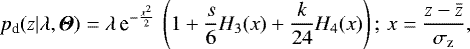
For the following galaxy-bias analysis, we estimate the probability density function (PDF) pd (z) of each galaxy sample from the mock catalogues in the foregoing step. Simply using histograms of the sample redshifts may seem like a good idea but is, in fact, problematic because the histograms depend on the adoptedbinning. This is especially relevant for the prediction of galaxy clustering that depends on  (see Eq. (22)). Instead, we fit for pd(z) a smooth four-parameter Gram-Charlier series
 (1)
(1)
with the Hermite polynomials H3(x) = x3 − 3x and H4(x) = x4 − 6x2 + 3 to a mock sample {zi: i = 1…n} of n galaxy redshifts; λ is a normalisation constant that depends on the parameter combination 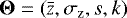 and is defined by
 (2)
(2)
For an estimate  of the parameters Θ, we maximise the log-likelihood
 (3)
(3)
with respect to Θ. This procedure selects the PDF  that is closest to the sample distribution of redshifts zi in a Kullback-Leibler sense (Knight 1999). The mean
  and variance
  in the fit matches that of the redshift distribution in the mock lens sample. The resulting densities for all our lens samples are shown in the two top panels of Fig. 1.
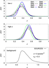 |
Fig. 1 Models of the probability densities pd(z) of galaxy redshifts in our lens samples SM1 to SM6, RED and BLUE (two top panels), and the density ps (z) of the source sample (bottom panel). |
2.2 Shear catalogues
For mock source catalogues based on the MS data, we construct lensing data by means of multiple-lens-plane ray tracing as described in Hilbert et al. (2009). The ray tracing produces the lensing convergence κ(θ |zs) and shear distortion γ(θ|zs) for 40962 line-of-sight directions θ on 64 regular angular grids and a sequence of ns = 31 source redshifts zs,i between zs = 0 and zs = 2; we denote by Δzi = zs,i+1 − zs,i the difference between neighbouring source redshifts. Each grid covers a solid angle of Ω =4 × 4 deg2. For each grid, we then compute the average convergence for sources with redshift PDF ps (z) by
 (4)
(4)
and the average shear γ(θ) from the sequence γ(θ|zs) accordingly. For ps(z), we employ the estimated PDF of CFHTLenS sources that is selected through i′ < 24.7 and 0.65 ≤ zp < 1.2, weighted by their shear-measurement error (SES13; see the bottom panel in Fig. 1). The mean redshift of sources is  . To assign source positions on the sky, we uniform-randomly pick a sample {θi: i = 1…n} of positions for each grid; the amount of positions is
  for a number density of
  sources, which roughly equals the effective number density of sources in SES13.
Depending on the type of our lensing analysis, we assign a source at θi of one of the following three values for the simulated sheared ellipticity ϵi: (i) ϵi = γ(θi) for source without shape noise; (ii) ϵi = A(γ(θi), ϵs) for noisy sources with shear; and (iii)  for noisy sources with reduced shear gi = γ(θi)∕[1 − κ(θi)]. We define here by
  the conformal mapping of two complex numbers x and y, and by ϵs a random shape noise drawn from a bivariate, truncated Gaussian PDF with zero mean, 1D dispersion σϵ = 0.3, and an exclusion of values beyond |ϵs|≥ 1.
2.3 Power spectra
We obtain the true spatial galaxy-galaxy, galaxy-matter, and matter-matter power spectra for all galaxy samples at a given simulation snapshot with fast Fourier transform (FFT) methods. For a choice of pair of tracers (i.e. simulation matter particles or galaxies from different samples) in a snapshot, we compute a series of raw power spectra by “chaining the power” (Smith et al. 2003). We cover the whole simulation volume as well as smaller sub-volumes (by a factor 43 to 2563, into which the whole box is folded) by regular meshes of 5123 points (providing a spatial resolution from ~1 h−1 Mpc for the coarsest mesh to ~5 h−1 kpc for the finest mesh). We project the tracers onto these meshes using clouds-in-cells (CIC) assignment (Hockney & Eastwood 1981).
We FFT-transform the meshes, record their raw power spectra, apply a shot-noise correction (except for cross-spectra), a deconvolution to correct for the smoothing by the CIC assignment, and an iterative alias correction (similar to what is described in Jing 2005). From these power spectra, we discard small scales beyond half their Nyquist frequency as well as large scales that are already covered by a coarser mesh, and combine them into a single power spectrum covering a range of scales from modes ~ 0.01 h Mpc−1 to modes ~ 100 h Mpc−1.
The composite power spectra are then used as input to estimate alias corrections for the partial power spectra from the individual meshes with different resolutions, and the process is repeated until convergence. From the resulting power spectra, we then compute the true biasing functions, Eq. (10), which we compare to our lensing-based reconstructions in Sect. 7.
3 Projected biasing functions as observed with lensing techniques
The combination of suitable statistics for galaxy clustering, galaxy-galaxy lensing, and cosmic-shear correlations on the sky allows us to infer, without a concrete physical model, the z-averaged spatial biasing functions b(k) and r(k) as projections b2D(θap) and r2D (θap) for varying angular scales θap. Later on, we forward-fit templates of spatial biasing functions to these projected functions to perform a stable de-projection. We summarise here the relation between (b(k), r(k)) and the observable ratio-statistics (b2D(θap), r2D(θap)). We include corrections to the first-order Born approximation for galaxy-galaxy lensing and galaxy clustering, and corrections for the intrinsic alignment of sources.
3.1 Spatial biasing functions
We define galaxy bias in terms of two biasing functions b(k) and r(k) for a given spatial scale 2π k−1 or wave number k in the following way. Let δ(x) in ![Mathematical equation: $\rho(\vec{x})=\overline{\rho}\,[1+\delta(\vec{x})]$](/articles/aa/full_html/2018/05/aa32248-17/aa32248-17-eq19.png) be the density fluctuations at position x of a random density field ρ(x), and
be the density fluctuations at position x of a random density field ρ(x), and  denotes the mean density. A density field is either the matter density ρm(x) or the galaxy number density ng(x) with densitycontrasts δm(x) and δg(x), respectively. We determine the fluctuation amplitude for a density mode k by the Fourier transform of δ(x),
 (5)
(5)
All information on the two-point correlations of  is contained in the power spectrum P(k) defined through the second-order correlation function of modes,
 (6)
(6)
where k = |k| is the scalar wave number and δD(s) is the Dirac Delta distribution. Specifically, we utilise three kinds of power spectra,
 (7) (8) (9)
namely the matter power spectrum Pm(k), the galaxy-matter cross-power spectrum Pgm(k), and the galaxy power spectrum Pg(k). The latter subtracts the shot noise  from the galaxy power spectrum by definition. In contrast to the smooth matter density, the galaxy number density is subject to shot noise because it consists of a finite number of discrete points that make up the number density field. Traditionally, the definition of Pg (k) assumes a Poisson process for the shot noise in the definition of Pg(k) (Peebles 1980).
The biasing functions (of the second order) express galaxy bias in terms of ratios of the foregoing power spectra,
 (10)
(10)
Galaxies that sample the matter density by a Poisson process have b(k) = r(k) = 1 for all scales k and are dubbed “unbiased”; for b(k) > 1, we find that galaxies cluster stronger than matter at scale k, and vice versa for b(k) < 1; a decorrelation of r(k)≠1 indicates either stochastic bias, non-linear bias, a sampling process that is non-Poisson, or combinations of these cases (Dekel & Lahav 1999; Guzik & Seljak 2001).
3.2 Aperture statistics and galaxy-bias normalisation
The projected biasing functions b(k) and r(k) are observable by taking ratios of the (co-)variances of the aperture mass and aperture number count of galaxies (van Waerbeke 1998; Schneider 1998). To see this, let 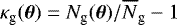 be the density contrast of the number density of galaxies Ng(θ) on the sky in the direction θ, and
 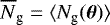 be their mean number density. We define the aperture number count of Ng (θ) for an angular scale θap at position θ by
 (11)
(11)
where
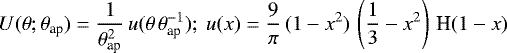 (12)
(12)
is the aperture filter of the density field, and H(x) is the Heaviside step function of our polynomial filter profile u(x). The aperture filter is compensated, that is  . Similarly for the (average) lensing convergence κ(θ) of sources in direction θ, the aperture mass is given by
 (13)
(13)
The aperture statistics consider the variances  and
and  of
of  and Map(θap;θ), respectively, across the sky, as well as their co-variance
  at zero lag.
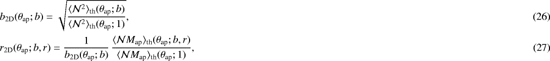
From these observable aperture statistics, we obtain the galaxy bias factor b2D (θap) and correlation factor r2D(θap) through the ratios
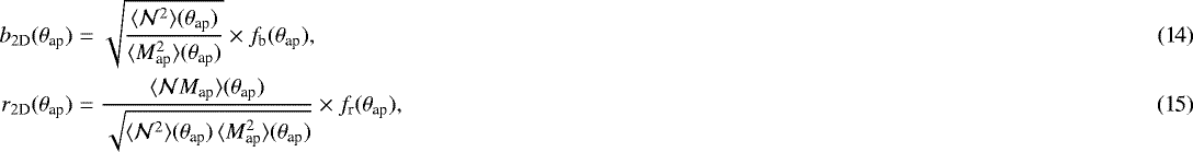 (14) (15)
where
 (16) (17)
normalise the statistics according to a fiducial cosmology, that means the aperture statistics with subscript “th” as in  denote the expected (co-)variance for a fiducial model. The normalisation is chosen such that we have b2D (θap) = r2D(θap) = 1 for unbiased galaxies given the distributions of lenses and sources with distance χ as in the survey, hence the “(θap;1)” in the arguments of the normalisation. The normalisation functions ff and fb are typically weakly varying withangular scale θap (Hoekstra et al. 2002). In addition, they depend weakly on the fiducial matter power spectrum Pm (k;z); they are even invariant with respect to an amplitude change Pm(k;z)↦υ Pm(k;z) with some number υ > 0. We explore the dependence on the fiducial cosmology quantitatively in Sect. 7.3.
For this study, we assume that the distance distribution of lenses is sufficiently narrow, which means that the bias evolution in the lens sample is negligible. We therefore skip the argument χ in b(k; χ) and r(k; χ), and we use a b(k) and r(k) independent of χ for average biasing functions instead.
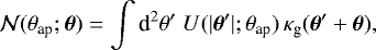
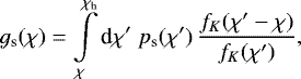
The relation between (b(k), r(k)) and (b2D(θap), r2D(θap)) is discussed in the following. Let pd(χ) dχ and ps(χ) dχ be the probability to find a lens or source galaxy, respectively, at comoving distance [χ, χ + dχ). The matter power spectrum at distance χ shall be Pm(k;χ), and  is a shorthand for the transverse spatial wave number k at distance χ that corresponds to the angular wave number ℓ. The function fK(χ) denotes the comoving angular-diameter distance in the given fiducial cosmological model. The additive constant 0.5 in
  applies a correction to the standard Limber approximation on the flat sky, which gives more accurate results for large angular scales (Kilbinger et al. 2017; Loverde & Afshordi 2008). According to theory, the aperture statistics are then
![Mathematical equation: \begin{align} & \langle {\mathcal{N}^2} \rangle_{\textrm{th}}({\theta}_{\textrm{ap}};b) = 2\pi\int\limits_0^{\infty}{\textrm{d}}\ell\,\ell\,P_{\textrm{n}}(\ell;b)\,\left[I(\ell{\theta}_{\textrm{ap}})\right]^2\!\!,\\ & \langle {\mathcal{N}M_{\textrm{ap}}} \rangle_{\textrm{th}}({\theta}_{\textrm{ap}};b,r) = 2\pi\int\limits_0^{\infty}{\textrm{d}}\ell\,\ell\,P_{\textrm{n}\kappa}(\ell;b,r)\,\left[I(\ell{\theta}_{\textrm{ap}})\right]^2\!\!,\\ &\langle {M_{\textrm{ap}}^2} \rangle_{\textrm{th}}({\theta}_{\textrm{ap}})= 2\pi\int\limits_0^{\infty}{\textrm{d}}\ell\,\ell\,P_{\kappa}(\ell)\,\left[I(\ell{\theta}_{\textrm{ap}})\right]^2\!\!,\end{align}](/articles/aa/full_html/2018/05/aa32248-17/aa32248-17-eq42.png) (18) (19) (20)
(18) (19) (20)
with the angular band-pass filter
 (21)
(21)
the angular power spectrum of the galaxy clustering
 (22)
(22)
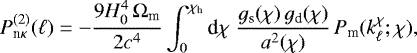
the galaxy-convergence cross-power
 (23)
(23)
and the convergence power-spectrum
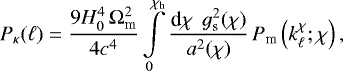 (24)
(24)
all in the Born and Limber approximation. In the integrals, we use the lensing kernel
 (25)
(25)
the scale factor a(χ) at distance χ, the maximum distance χh of a source, and the nth-order Bessel function Jn(x) of the first kind. By c we denote the vacuum speed of light. The power spectra and aperture statistics depend on specific biasing functions as indicated by the b and r in the arguments. For given biasing functions b(k) and r(k), we obtain the normalised galaxy bias inside apertures therefore through
 (26) (27)
which can be compared to measurements of Eqs. (14) and (15).
3.3 Intrinsic alignment of sources
Recent studies of cosmic shear find evidence for an alignment of intrinsic source ellipticities that contribute to the shear-correlation functions (Hildebrandt et al. 2017; Abbott et al. 2016; Troxel & Ishak 2015; Heymans et al. 2013; Joachimi et al. 2011; Mandelbaum et al. 2006). These contributions produce systematic errors in the reconstruction of b(k) and r(k) if not included in their normalisation fb and fr. Relevant are “II”-correlations between intrinsic shapes of sources in  and “GI”-correlations between shear and intrinsic shapes in both
  and
and  . The GI term in
  can be suppressed by minimising the redshift overlap between lenses and sources. Likewise, the II term is suppressed by a broad redshift distribution of sources which, however, increases the GI amplitude. The amplitudes of II and GI also vary with galaxy type and luminosity of the sources (Joachimi et al. 2011).
An intrinsic alignment (IA) of sources has an impact on the ratio statistics b2D (θap) and r2D (θap), Eqs. (14) and (15), mainly through  if we separate sources and lenses in redshift. The impact can be mitigated by using an appropriate model for
  and
and  in the normalisation of the measurements. For this study, we do not include II or GI correlations in our synthetic mock data but, instead, predict the amplitude of potential systematic errors when ignoring the intrinsic alignment for future applications in Sect. 7.3.
For a reasonable prediction of the GI and II contributions to  , we use the recent non-evolution model utilised in Hildebrandt et al. (2017). This model is implemented by using
 (28)
(28)
instead of (24) in Eq. (20). The new II and GI terms are given by
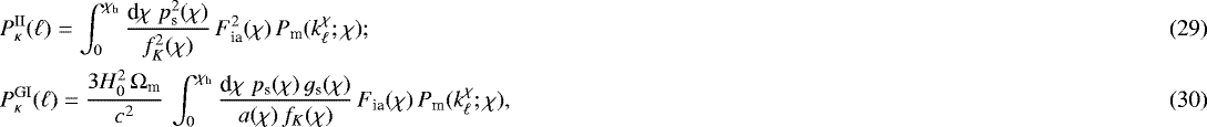 (29) (30)
where
 (31)
(31)
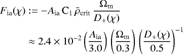
controls the correlation amplitude in the so-called “non-linear linear” model (see Hirata & Seljak 2004; Bridle & King 2007; or Joachimi et al. 2011; for details). The factor Aia scales the amplitude; it broadly falls within Aia ∈ [−3, 3] for recent cosmic-shear surveys and is consistent with Aia ≈ 2 for sources in the Kilo-Degree Survey (Joudaki et al. 2018; Hildebrandt et al. 2017; Heymans et al. 2013). For the normalisation of Fia (χ), we use  , and the linear structure-growth factor D+(χ), normalised to unity for χ = 0 (Peebles 1980). By comparing
  and Pn(ℓ) in Eq. (22) we see that II contributions are essentially the clustering of sources on the sky (times a small factor). Likewise,
  is essentially the correlation between source positions and their shear on the sky (cf. Eq. (23)). In this IA model, we assume a scale-independent galaxy bias for sources in the IA modelling since Fia (χ) does not depend on k.
In Fig. 2, we plot the predicted levels of II and GI terms in the observed  for varying values of Aia as black and red lines for our MS cosmology and the ps(z) in our mock survey. The corresponding value of Aia is shown asa number in the figure key. We use negative values of Aia for GI to produce positive correlations for the plot; the corresponding predictions for − Aia have the same amplitude as those for Aia but with opposite sign. The II terms, on the other hand, are invariant with respect to a sign flip of Aia. All curves in the plot use a matter power spectrum Pm(k;χ) computed with Halofit (Smith et al. 2003) and the update in Takahashi et al. (2012). For comparison, we plot as blue line GG the theoretical
  without GI and II terms. For |Aia|≈ 3, GI terms can reach levels up to 10% to 20% of the correlation signal for θap ≳ 1′, whereas II terms are typically below 10%. The GI and II terms partly cancel each other for Aia > 0 so that the contamination is worse for negative Aia.
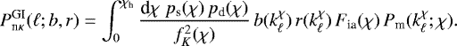
Moreover, we quantify the GI term in  by using in (19) the modified power spectrum
 (32)
(32)
with
 (33)
(33)
This is the model in Joudaki et al. (2018; see their Eq. (11)) with an additional term  that accounts for a decorrelation of the lens galaxies. This GI model is essentially the relative clustering between lenses and unbiased sources on the sky and therefore vanishes in the absence of an overlap between the lens and source distributions, which means that ∫ dχ ps(χ) pd(χ) = 0. In Fig. 3, we quantify the relative change in
  owing to the GI term for different values of Aia. Since the change is very similar for all galaxy samples in the same redshift bin, we plot only the results for SM4. The overlap between sources and lenses is only around 4% for low-z samples and, therefore, the change stays within 2% for all angular scales considered here (SES13). On the other hand, for high-z samples where we have roughly 14% overlap between the distributions, the change can amount to almost 10% for Aia ≈±2 and could have a significant impact on the normalisation.
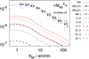 |
Fig. 2 Levels of GI and II contributions to |


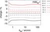 |
Fig. 3 Relative change of |

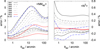 |
Fig. 4 Relative errors in the aperture statistics due to magnification bias of the lenses. Left: errors for |


3.4 Higher-order corrections
Corrections to the (first-order) Born approximation or for the magnification of the lenses cannot always be neglected as done in Eq. (23) (e.g. Ziour & Hui 2008; Hilbert et al. 2009; Hartlap 2009). This uncorrected equation over-predicts the power spectrum Pnκ(ℓ) by up to 10% depending on the galaxy selection and the mean redshift of the lens sample; the effect is smaller in a flux-limited survey but also more elaborate to predict as it depends on the luminosity function of the lenses. Hilbert et al. (2009) tests this for the tangential shear around lenses by comparing (23) to the full-ray-tracing results in the MS data, which account for contributions from lens-lens couplings and the magnification of the angular number density of lenses.
For a volume-limited lens sample, Hartlap (2009, H09 hereafter), derives the second-order correction (in our notation)
 (34)
(34)
where
 (35)
(35)
for a more accurate power spectrum  that correctly describes the correlations in the MS. Physically, this correction accounts for the magnification of the projected number density of lens galaxies by matter in the foreground. We find that the thereby corrected
  can be different to the uncorrected aperture statistic by up to a few % (see left-hand panel in Fig. 4). This directly affects the normalisation of r2D (θap): the measured, normalised correlation r2D(θap) would be systematically low. We obtain Fig. 4 by comparing the uncorrected to the corrected
  for each of our lens-galaxy samples. In accordance with H09, we find that the systematic error is not negligible for some lens sample, and we therefore include this correction by employing
  instead of Pn κ (ℓ) in the normalisation fr (θap) and in the prediction r2D (θap;b, r). This improves the accuracy of the lensing reconstruction of r(k) by up to a few %, most notably the sample blue high-z, especially around k ≈ 1 h Mpc−1, which corresponds to θap ≈ 10′.
Additional second-order terms for Pnκ(ℓ) arise due to a flux limit of the survey (Eqs. (3.129) and (3.130) in H09), but they require a detailed model of the luminosity function for the lenses. We ignore these contributions here because our mock lens samples, selected in redshift bins of Δ z ≈ 0.2 and for stellar masses greater than 5 × 10⁹ M⊙, are approximately volume limited because of the lower limit of stellar masses and the redshift binning (see Sect. 4.1 in Simon et al. 2017, which uses our lens samples).
Similarly, by
 (36)
(36)
H09 gives a second-order correction for Pn(ℓ;b) in addition to more corrections for flux-limited surveys (Eqs. (3.140)–(3.143)). We include  by using
  instead of Eq. (22) in the following for fb(θap) and b2D(θap;b, r), although this correction is typically below half a % here (see the right-hand panel in Fig. 4).
4 Model templates of biasing functions
Apart from the galaxy-bias normalisation, the ratio statistics b2D and r2D are model-free observables of the spatial biasing functions, averaged for the radial distribution of lenses. The de-projection of the ratio statistics into (an average) b(k) and r(k) is not straightforward due to the radial and transverse smoothing in the projection. Therefore, for a de-projection we construct a parametric family of templates that we forward-fit to the ratio statistics. In principle, this family could be any generic function but we find that physical templates that can be extrapolated to scales unconstrained by the observations result in a more stable de-projection. To this end, we pick a template prescription that is motivated by the halo-model approach but with more freedom than is commonly devised (Cooray & Sheth 2002, for a review). Notably, we derive explicit expressions for b(k) and r(k) in a halo-model framework.
4.1 Separation of small and large scales
Before we outline the details of our version of a halo model, used to construct model templates, we point out that any halo model splits the power spectra Pm(k), Pgm(k), and Pg (k) into one- and two halo terms,
 (37)
(37)
The one-halo term P1h(k) dominates at small scales, quantifying the correlations between density fluctuations within the same halo, whereas the two-halo term P2h (k) dominates the power spectrum at large scales where correlations between fluctuations in different halos and the clustering of halos become dominant.
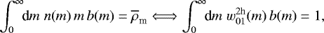
We exploit this split to distinguish between galaxy bias on small scales (one-halo terms) and galaxy bias on large scales (two-halo terms), namely
 (38)
(38)
and
 (39)
(39)
and we derive approximations for both regimes separately. We find that the two-halo biasing functions are essentially constants, and the one-halo biasing functions are only determined by the relation between matter and galaxy density inside halos.
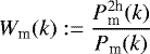
To patch together both approximations of the biasing functions in the one-halo and two-halo regime, we then do the following. Based on Eq. (10), the function b2 (k) is a weighted mean of b1h(k) and b2h(k):
![Mathematical equation: \begin{eqnarray*} \nonumber b^2(k)&=& \frac{P^{1\textrm{h}}_{\textrm{g}}(k)+P^{2\textrm{h}}_{\textrm{g}}(k)} {P_{\textrm{m}}(k)} \\ \nonumber&=& \frac{P^{1\textrm{h}}_{\textrm{m}}(k)\,[b^{1\textrm{h}}(k)]^2} {P_{\textrm{m}}(k)} + \frac{P^{2\textrm{h}}_{\textrm{m}}(k)\,[b^{2\textrm{h}}(k)]^2 } {P_{\textrm{m}}(k)} \\&=& \Big(1-W_{\textrm{m}}(k)\Big)\,[b^{1\textrm{h}}(k)]^2+W_{\textrm{m}}(k)\,[b^{ 2\textrm{h}}(k)]^2, \end{eqnarray*}](/articles/aa/full_html/2018/05/aa32248-17/aa32248-17-eq82.png) (40)
(40)
where the weight
 (41)
(41)
is the amplitude of the two-halo matter power spectrum relative to the total matter power spectrum. Deep in the one-halo regime we have Wm(k) ≈ 0 but Wm(k) ≈ 1 in the two-halo regime. Since the two-halo biasing is approximately constant, the scale dependence of galaxy bias is mainly a result of the galaxy physics inside halos and the shape of Wm(k).
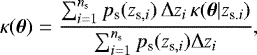
Once the weight Wm(k) is determined for a fiducial cosmology, it does not rely on galaxy physics and we can use it for any model of b1h (k) and b2h (k). In principle, the weight Wm(k) could be accurately measured from a cosmological simulation by correlating only the matter density from different halos for  , which is then normalised by the full power spectrum Pm(k) in the simulation. We, however, determine Wm(k) by computing the one-halo and two-halo term of Pm(k) with the setup of Simon et al. (2009). Our results for Wm(k) at different redshifts are plotted in Fig. 5. There we find that the transition between the one-halo and two-halo regime, Wm ~ 0.5, is at k ~ 0.3 h Mpc−1 for z = 0, whereas the transition point moves to k ~ 1 h Mpc−1 for z ~ 1.
Similar to b(k), we can expand the correlation function r(k) in terms of its one-halo and two-halo biasing functions. To this end, let
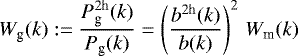 (42)
(42)
be a weight by analogy to Wm(k). For unbiased galaxies, that is b2h(k) = b(k) = 1, we simply have Wg(k) = Wm(k). Using the definition of r(k) in Eq. (10) and Eq. (39), we generally find
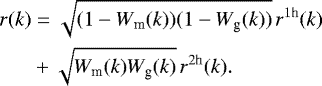 (43)
(43)
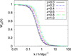 |
Fig. 5 Weight Wm(k) of the two-halo term in the matter-power spectrum for varying redshifts z. |
4.2 Halo-model definitions
For approximations of the biasing functions in the one- and two-halo regime, we apply the formalism in Seljak (2000) and briefly summarise it here. All halo-related quantities depend on redshift. In the fits with the model later on, we use for this the mean redshift of the lens galaxies.
We shall denote by n(m) dm the (comoving) number density of halos within the halo-mass range [m, m + dm); ⟨N|m⟩ is the mean number of galaxies inside a halo of mass m; ⟨N(N − 1)|m⟩ is the mean number of galaxy pairs inside a halo of mass m. Let u(r, m) be the radial profile of the matter density inside a halo or the galaxy density profile. Also let
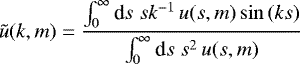 (44)
(44)
be its normalised Fourier transform. Owing to this normalisation, profiles obey ũ (k, m) = 1 at k = 0. To assert a well-defined normalisation of halos, we truncate them at their virial radius rvir, which we define by the over density  within the distance rvir from the halo centre and by Δvir(z) as in Bullock et al. (2001). Furthermore, the mean matter and galaxy number density (comoving) are
 (45)
(45)
The one-halo terms of the galaxy power spectrum Pg(k), the matter power spectrum Pm(k), and the galaxy-matter cross-power spectrum Pgm(k) are
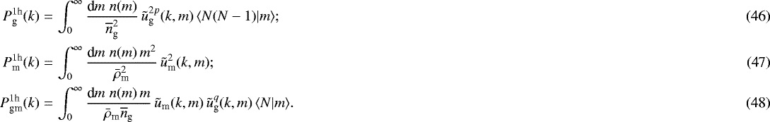 (46) (47) (48)
In these equations, the exponents p and q are modifiers of the statistics for central galaxies, which are accounted for in the following simplistic way: central galaxies are by definition at the halo centre r = 0; one galaxy inside a halo is always a central galaxy; their impact on galaxy power spectra is assumed to be only significant for halos that contain few galaxies. Depending on whether a halo contains few galaxies or not, the factors (p, q) switch on or off a statistics dominated by central galaxies through
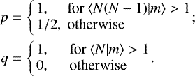 (49)
(49)
We note that p and q are functions of the halo mass m. Later in Sect. 4.6, we consider also more general models where there can be a fraction of halos that contains only satellite galaxies. We achieve this by mixing (46)–(48) with power spectra in a pure-satellite scenario, this means a scenario where always p ≡ q ≡ 1.
We now turn to the two-halo terms in this halo model. We approximate the clustering power of centres of halos with mass m by  , where Plin(k) denotes the linear matter power spectrum, and bh(m) is the halo bias factor on linear scales; the clustering of halos is thus linear and deterministic in this description. Likewise, this model approximates the cross-correlation power-spectrum of halos with the masses m1 and m2 by bh (m1) bh(m2) Plin(k). The resulting two-halo terms are then
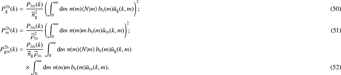 (50) (51) (52)
The two-halo terms ignore power from central galaxies because it is negligible in the two-halo regime.
4.3 A toy model for the small-scale galaxy bias
We first consider an insightful toy model of b(k) and r(k) at small scales. In this model, both the matter and the galaxy distribution shall be completely dominated by halos of mass m0, such that we find an effective halo-mass function n(m) ∝ δD(m − m0); its normalisation is irrelevant for the galaxy bias. In addition, the halos of the toy model shall not cluster so that the two-halo terms of the power spectra vanish entirely. The toy model has practical relevance in what follows later because the one-halo biasing functions that we derive afterwards are weighted averages of toy models with different m0. For this reason, most of the features can already be understood here, albeit not all, and it already elucidates biasing functions on small scales.
Let us define the variance  of the halo-occupation distribution (HOD) in excess of a Poisson variance ⟨N|m0⟩ by
 (53)
(53)
If the model galaxies obey Poisson statistics, they have  . We can nowwrite the mean number of galaxy pairs as
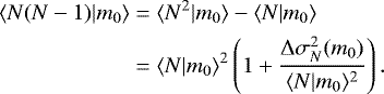 (54)
(54)
By using Eqs. (46)–(48) with n(m) ∝ δD(m − m0), the correlation factor reads
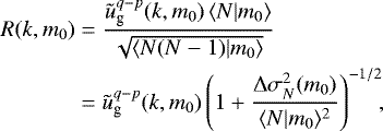 (55)
(55)
and the bias factor is
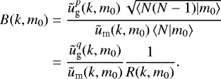 (56)
(56)
To avoid ambiguities in the following, we use capital letters for the biasing functions in the toy model.
We dub galaxies “faithful tracers” of the matter density if they have both (i) ũg (k, m) = ũm(k, m) and (ii) no central galaxies (p = q = 1). Halos with relatively small numbers of galaxies, that is ⟨N|m0⟩, ⟨N(N − 1)|m0⟩≲ 1, are called “low-occupancy halos” in the following. This toy model then illustrates the following points.
-
Owing to galaxy discreteness, faithful tracers are biased if they not obey Poisson statistics. Namely, for a sub-Poisson variance,
 , they produce opposite trends R(k, m0) > 1 and B(k, m0) < 1 with k, and vice versa for a super-Poisson sampling, but generally we find the relation R(k, m0) × B(k, m0) = 1.
 -
Nevertheless faithful tracers obey B(k, m0), R(k, m0) ≈ 1 if the excess variance becomes negligible, that is if
 . The discreteness of galaxies therefore becomes only relevant in low-occupancy halos.
 -
A value of R(k, m0) > 1 occurs once central galaxies are present (p, q < 1). As a central galaxy is always placed at the centre, central galaxies produce a non-Poisson sampling of the profile um(r, m0). In contrast to faithful galaxies with a non-Poisson HOD, we then find agreeing trends with scale k for R(k, m0) and B(k, m0) if
 . Again, this effect is strong only in low-occupancy halos.
 -
The biasing functions in the toy model are only scale-dependent if galaxies are not faithful tracers. The bias function B(k, m0) varies with k if either ũm(k, m0)≠ũg(k, m0) or for central galaxies (p≠1). The correlation function R(k, m0) is scale-dependent only for central galaxies, that is p − q≠0, which then obeys
 . Variations with k become small for both functions, however, if ũm(k, m0), ũg(k, m0) ≈ 1, which is on scales larger than the size rvir of a halo.
We stress again that a counter-intuitive r(k) > 1 is a result of the definition of Pg(k) relative to Poisson shot-noise and the actual presence of non-Poisson galaxy noise. One may wonder here if r > 1 is also allowed for biasing parameters defined in terms of spatial correlations rather than the power spectra. That this is indeed the case is shown in Appendix A for completeness.
4.4 Galaxy biasing at small scales
Compared to the foregoing toy model, no single halo mass scale dominates the galaxy bias at any wave number k for realistic galaxies. Nevertheless, we can express the realistic biasing functions b1h (k) and r1h (k) in the one-halo regime as weighted averages of the toy model B(k, m) and R(k, m) with modifications.
To this end, we introduce by
 (57)
(57)
the “mean biasing function”, which is the mean number of halo galaxies ⟨N|m⟩ per halo mass m in units of the cosmic average  (Cacciato et al. 2012). If galaxy numbers linearly scale with halo mass, that means ⟨N|m⟩∝ m, we find a mean biasing function of b(m) = 1, while halos masses devoid of galaxies have b(m) = 0. For convenience, we make useof ⟨N|m⟩∝ m b(m) instead of ⟨N|m⟩ in the following equations because we typically find ⟨N|m⟩∝ mβ with β ≈ 1: b(m) is therefore usually not too different from unity.
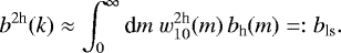
Using Eqs. (46) and (47) we then find
![Mathematical equation: \begin{equation*}[b^{1\textrm{h}}(k)]^2= \frac{P^{1\textrm{h}}_{\textrm{g}}(k)}{P^{1\textrm{h}}_{\textrm{m}}(k)} = \int_0^{\infty}{\textrm{d}} m\;w_{20}^{1\textrm{h}}(k,m)\, b^2(m)\,B^2(k,m), \end{equation*}](/articles/aa/full_html/2018/05/aa32248-17/aa32248-17-eq106.png) (58)
(58)
with  being one case in a family of (one-halo) weights,
![Mathematical equation: \begin{equation*} w_{ij}^{1\textrm{h}}(k,m):= \frac{n(m)\,m^2\,\tilde{u}_{\textrm{m}}^i(k,m)\,[b(m)\,\tilde{u}_{\textrm{g}}(k,m)]^j} {\int_0^{\infty}\!\textrm{d} m\;n(m)\,m^2\,\tilde{u}_{\textrm{m}}^i(k,m)\,[b(m)\,\tilde{u}_{\textrm{g}}(k,m)]^j}. \end{equation*}](/articles/aa/full_html/2018/05/aa32248-17/aa32248-17-eq108.png) (59)
(59)
This family and the following weights w(k, m) are normalised, which means that ∫ dm w(k, m) = 1. The introduction of these weight functions underlines that the biasing functions are essentially weighted averages across the halo mass spectrum as, for example, ![Mathematical equation: $[b^{1\textrm{h}}(k)]^2$](/articles/aa/full_html/2018/05/aa32248-17/aa32248-17-eq109.png) , which is the weighted average of b2(m) B2(k, m).
, which is the weighted average of b2(m) B2(k, m).
The effect of  is to down-weight large halo masses in the bias function because
  decreases with m1 for a fixed m2 < m1 and k. Additionally, the relative weight of a halo with mass m decreases towards larger k because ũm(k, m) tends to decrease with k. As a result, at a given scale k only halos below a typical mass essentially contribute to the biasing functions (Seljak 2000).
We move on to the correlation factor r1h(k) in the one-halo regime. Using Eqs. (46)–(48) and the relations
 (60) (61) (62)
we write
 (63)
(63)
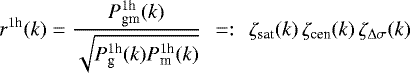
as product of the three separate factors
 (64) (65) (66)
with the following meaning:
-
The first factor ζsat(k) quantifies, at spatial scale k, the correlation between the radial profiles of the matter density
 and the (average) number density of satellite galaxies
  across the halo mass spectrum n(m). As upperbound we always have |ζsat(k)|≤ 1 because of the Cauchy-Schwarz inequality when applied to the nominator of Eq. (64). Thus ζsat(k) probably reflects best what we intuitively understand by a correlation factor between galaxies and matter densities inside a halo. Since it only involves the average satellite profile, the satellite shot-noise owing to a HOD variance is irrelevant at this point. The next two factors can be seen as corrections to ζsat(k) owing tocentral galaxies or a non-Poisson HOD variance.
 -
The second factor ζcen(k) is only relevant in the sense of ζcen(k)≠1 through low-occupancy halos with central galaxies (q≠1). It has the lower limit ζcen(k) ≥ 1 because of ũg(k, m) ≤ 1 and hence
 . This correction factor can therefore at most increase the correlation r1h(k).
 -
The third factor ζΔσ(k) is the only one that is sensitive to an excess variance
 of the HOD, namely through R(k, m). In the absence of central galaxies, that means for p ≡ q ≡ 1,
  is the (weighted) harmonic mean of R2(k, m), or the harmonic mean of the reduced
 ![Mathematical equation: $[\tilde{u}_{\textrm{g}}(k,m)\,R(k,m)]^2\le R^2(k,m)$](/articles/aa/full_html/2018/05/aa32248-17/aa32248-17-eq120.png) otherwise.
otherwise.
As sanity check, we note the recovery of the toy model by setting n(m) ∝ δD(m − m0) in (58) and (63). In contrast to the toy model, the templates b1h (k) and r1h (k) can be scale-dependent even if B(k, m) and R(k, m) are constants. This scale dependence can be produced by a varying  or ζsat(k).
4.5 Galaxy biasing at large scales
From the two-halo terms (50)–(52), we can immediately derive the two-halo biasing functions. The bias factor is
 (67)
(67)
where we have introduced into the integrals the normalised (two-halo) weights
![Mathematical equation: \begin{equation*} w_{ij}^{2\textrm{h}}(m):= \frac{n(m)\,[m\,b(m)]^i\,m^j}{\int_0^{\infty}{\textrm{d}} m\;n(m)\,[m\,b(m)]^i\,m^j}. \end{equation*}](/articles/aa/full_html/2018/05/aa32248-17/aa32248-17-eq123.png) (68)
(68)
We additionally approximate ũ(k, m) ≈ 1 for the two-halo regime. This is a reasonable approximation because virialised structures are typically not larger than ~ 10 h−1 Mpc and hence exhibit ũ(k, m) ≈ 1 for k ≪ 0.5 h Mpc−1. Therefore, we find an essentially constant bias function at large scales,
 (69)
(69)
We have used here  , which follows from the constraint Pm(k) → Plin(k) for k → 0 and Eq. (51). To have more template flexibility, we leave bls as a free parameter and devise Eq. (69) only if no large-scale information is available by observations.
The two-halo correlation function at large scales is exactly
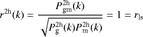 (70)
(70)
due to Ph(k;m1, m2) = bh(m1) bh(m2) Pm(k) for the assumed halo clustering. Evidently, the large-scale matter-galaxy correlation is fixed to rls = 1. The correlation is necessarily high because the model galaxies are always inside halos so that galaxies closely follow the matter distribution at large scales.
We notethat rls≠1 is physically conceivable although it is usually excluded in halo models (Tegmark & Peebles 1998). To test for an actually high correlation rls = 1 in real data, we may use rls as a free parameter in the templates.
4.6 Fraction of central galaxies
Up to here, we assumed either one central galaxy for every halo that hosts galaxies or pure samples of satellite galaxies, meaning p ≡ q ≡ 1. In reality where we select sub-populations of galaxies, not every sub-sample automatically provides a central galaxy in every halo; a central galaxy could belong to another galaxy population, for instance. For more template flexibility, we thus assume that only a fraction fcen of halos can have central galaxies from the selected galaxy population; the other fraction 1 − fcen of halos has either only satellites or central galaxies from another population. Both halo fractions nevertheless shall contain ⟨N|m⟩ halo galaxies on average. Importantly, fcen shall be independent of halo mass. This is not a strong restriction because the impact of central galaxies becomes only relevant for low-occupancy halos whose mass scale m is confined by ⟨N|m⟩≲ 1 anyway.
The extra freedom of fcen≠1 in the templates modifies the foregoing power spectra. On the one hand, the two-halo power spectra are unaffected because they do not depend on either p or q. On the other hand, for the one-halo regime, we now find the linear combination
 (71) (72)
because halos with (or without) central galaxies contribute with probability fcen (or 1 − fcen) to the one-halo term. In Eqs. (71) and (72) the Pcen(k) denote the one-halo power spectra of halos with central galaxies, and the Psat(k) denote spectra of halos with only satellites. Both cases are covered in the foregoing formalism for appropriate values of p, q: satellite-only halos with superscript “sat” are obtained by using p ≡ q ≡ 1; halos with central galaxies, superscript “cen”, use the usual mass-dependent expressions (49).
As result, we can determine the bias factor for the mixture scenario with (71) by
![Mathematical equation: \begin{equation*}[b^{1\textrm{h}}(k)]^2= f_{\textrm{cen}}\,[b_{\textrm{cen}}(k)]^2 + (1-f_{\textrm{cen}})\,[b_{\textrm{sat}}(k)]^2. \end{equation*}](/articles/aa/full_html/2018/05/aa32248-17/aa32248-17-eq128.png) (73)
(73)
Here bcen(k) denotes Eq. (58) in the central-galaxy scenario, whereas bsat(k) denotes the satellite-only scenario of this equation. Similarly for the correlation r1h (k) we obtain with (71) and (72)
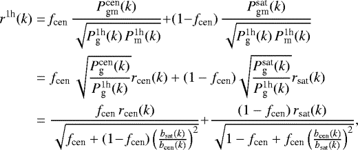 (74)
(74)
because
![Mathematical equation: \begin{equation*} P_{\textrm{g}}^{1\textrm{h}}(k)= f_{\textrm{cen}}\,[b_{\textrm{cen}}(k)]^2\,P^{1\textrm{h}}_{\textrm{m}}(k)+ (1-f_{\textrm{cen}})\,[b_{\textrm{sat}}(k)]^2\,P^{1\textrm{h}}_{\textrm{m}}(k). \end{equation*}](/articles/aa/full_html/2018/05/aa32248-17/aa32248-17-eq130.png) (75)
(75)
The function rcen(k) denotes Eq. (63) in the central-galaxy scenario, and rsat(k) is the satellite-only scenario.
5 Parameters of model templates and physical discussion
In this section, we summarise the concrete implementation of our templates, and we discuss their parameter dependence for a physical discussion on the scale-dependent galaxy bias.
5.1 Normalised excess variance
For a practical implementation of our templates, we find it useful to replace  in Eq. (53) by the “normalised excess variance”
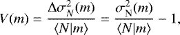 (76)
(76)
which typically has a small dynamic range with values between minus and plus unity. To see this, we discuss its upper and lower limits in the following.
First, the normalised excess variance has a lower limit because the average number of galaxy pairs is always positive,
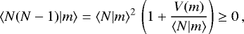 (77)
(77)
which imposes V (m) ≥−⟨N|m⟩. As additional constraint we have a positive variance
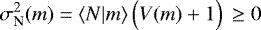 (78)
(78)
or V(m) ≥−1, so that we use
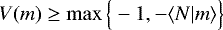 (79)
(79)
for a valid set of template parameters.
Second for the upper limit of V (m), we imagine that there is a maximum Nmax(m) for the amount of halo galaxies (of the selected population) inside a halo of mass m. A maximum Nmax(m) makes physical sense because we cannot squeeze an arbitrary number of galaxies into a halo. Nevertheless, their amount 0 ≤ N(m) ≤ Nmax(m) will be random with PDF P(N|m). Of this PDF we already know that its mean is ⟨N|m⟩. For its the maximum possible variance  , we note that
  cannot be larger than that for halos with a bimodal distribution of only two allowed galaxy numbers N(m) ∈{0, Nmax(m)} that shall occur with probability 1 −λ and λ, respectively. The mean of this bimodal PDF is ⟨N|m⟩ = λ Nmax(m), and its variance
  consequently satisfies
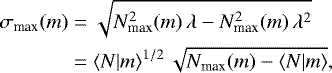 (80)
(80)
which is the upper limit for any P(N|m). Together with the lower bound of V (m), we thus arrive at
 (81)
(81)
This means that halos that are (on average) filled close to the limit, that is ⟨N|m⟩≈ Nmax(m) ≥ 1, have a HOD variance that is sub-Poisson,close to V (m) = −1. This should be especiallythe case for halos with ⟨N|m⟩≈ 1. On the other hand, halos with Nmax(m) ≈ 1 and low occupancy, ⟨N|m⟩≪ 1, necessarily obey Poisson statistics or are close to that, which means that V (m) ≈ 0. On the other extreme end, spacious halos well below the fill limit, Nmax(m) ≫ 1 and Nmax(m) ≫⟨N|m⟩, have sufficient headroom to allow for a super-Poisson variance, which means that V (m) > 0. In the following, we adopt the upper limit V (m) ≤ +1 meaning that we a priori do not allow the HOD variance to become larger than twice the Poisson variance.
List of free template parameters.
5.2 Implementation
Generally the functions V (m) and b(m) are continuous functions of the halo mass m. We apply, however, an interpolation with 20 interpolation points on a equidistant logarithmic m-scale for these functions, spanning the range 108 h−1 M⊙ to 1016 h−1 M⊙; between adjacent sampling points we interpolate linearly on the log-scale; we set b(m) = V (m) = 0 outside the interpolation range. Additionally, we find in numerical experiments with unbiased galaxies that the halo mass scale has to be lowered to 104 h−1 M⊙ to obtain correct descriptions of the bias. We therefore include two more interpolation points at 104 and 106 h−1 M⊙ to extend the mass scale to very low halo masses. For the large-scale bias, we set rls ≡ 1 but leave bls as a free parameter.
To predict the number density  of galaxies, Eq. (45), and to determine (p, q) for a given mass m, we have to obtain ⟨N|m⟩ from b(m). For this purpose, we introduce another parameter mpiv, which is the pivotal mass of low-occupancy halos, defined by ⟨N|mpiv⟩ = 1 such that
 (82)
(82)
The (comoving) number density of galaxies  is then given by
 (83)
(83)
for which we use  . With this parameterisation, the normalisation of b(m) is irrelevant in all equations of our bias templates. Nevertheless, b(m) can be shown to obey
 (84)
(84)
which follows from Eqs. (57) and (45). When plotting b(m), we make sure that it is normalised correspondingly.
Furthermore for the templates, we assume that satellite galaxies always trace the halo matter density so that ũg (k, m) ≡ũm(k, m). This assumption could be relaxed in a future model extension. For the matter density profile ũm(k, m), we assume an Navarro-Frenk-White profile (Navarro et al. 1996) with a mass concentration as in Seljak (2000) and a halo mass spectrum n(m) according to Sheth & Tormen (1999). For the average biasing functions b(k) and r(k), we evaluate n(m), bh (m), and ũm(k, m) at the mean redshift of the lens galaxies. As a model for Pm(k;χ) in Sect. 3.2 we employ the publicly available code nicaea2 version 2.5 (Kilbinger et al. 2009) that provides an implementation of Halofit with the recent update by Takahashi et al. (2012) and the matter transfer function in Eisenstein & Hu (1998) for baryonic oscillations.
We list all free parameters of the templates in Table 2. Their total number is 47 by default. In a future application, we may also consider rls a free parameter to test, for instance, the validity of rls = 1. If no large-scale information on the aperture statistics is available, we predict bls from Eq. (69), reducing the degrees of freedom in the model by one.
To obtain the biasing functions b(k) and r(k) from the set of parameters, we proceed as follows. We first compute the one-halo terms (58) and (63) for two separate scenarios: with and without central galaxies. Both scenarios are then mixed according to Eqs. (73) and (74) for the given value of fcen. Finally, we patch together the one- and two-halo biasing functions according to Eqs. (43) and (40) with a weight Wm(k) for the fiducial cosmology.
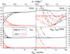 |
Fig. 6 Family of templates b(k) (black lines) and r(k) (red lines) for the range of wave numbers k in the top axis; the left-hand y axis applies to the panels in the first column, the right-hand axis to the second column. The aperture scale θap = 4.25∕(k fK(zd)) (bottom axis) crudely traces the projected b2D(θap) and r2D(θap) for lens galaxies at zd = 0.3. Each panel varies only one template parameter. See text for more details. |
5.3 Physical discussion
Figure 6 is a showcase of conceivable biasing functions and their relation to the underlying galaxy physics, which we compute in the aforementioned way. The wave number k is plotted on the top axis, whereas the bottom axis is defined by θap = 4.25∕(k fK(zd)) for a lens redshift of zd = 0.3, which is essentially a simplistic prediction for b2D(θap) and r2D(θap) as observed by the lensing technique in Sect. 3. For the discussion here, we concentrate on the spatial biasing functions.
We plot both b(k) and r(k) inside each panel. The black lines show a family of b(k) that we obtain by varying one template parameter at a time in a fiducial model; the red lines are families of r(k). The varied parameter is indicated in the top right corner of each panel. We assume a large-scale bias bls according to Eq. (69) with the theoretical halo bias bh(m) in Tinker et al. (2005). The fiducial model has: (i) no central galaxies, fcen = 0; (ii) a constant b(m) > 0 for m ∈ [109, 1015] h−1 M⊙ but vanishing everywhere else; (iii) a Poisson HOD-variance, V (m) = 0, for all halo masses; and (iv) a pivotal mass of mpiv = 1011 h−1 M⊙. This setup results in a large-scale bias factor of bls = 1.48. The details of the panels are as follows.
-
The bottom left panel varies fcen between zero and 100% in steps of 20% (bottom to top lines). Affected by a change of fcen are only the small scales k ≳ 10 h−1 Mpc (or θap ≲ 1 arcmin) that are strongly influenced by low-mass, low-occupancy halos.
-
The bottom right panel increases mpiv from 109 h−1 M⊙ (bottom line) to 1013 h−1 M⊙ (top line) in steps of one dex. An impact on the bias functions is only visible if we have either a non-Poisson HOD variance or central galaxies. We hence set fcen = 20% compared to the fiducial model. A greater value of mpiv shifts the mass scale of low-occupancy halos to larger masses and thus their impact on the bias functions to larger scales.
-
In the top left panel, we adopt a sub-Poisson model of V (m) = max{−0.5, −⟨N|m⟩} for halos with m ≤ mv. We step up the mass scale mv from 1010 h−1 M⊙ (bottom line for r; top line for b) to 1014 h−1 M⊙ (top line for r; bottom line for b) in one dex steps. Similar to the toy model in Sect. 4.3, a sub-Poisson variance produces opposite trends for b and r: if b goes up, r goes down, and vice versa. The effect is prominent at small scales where low-occupancy halos significantly contribute to the bias functions. Conversely to what is shown here, these trends in b and r change signs if we adopt a super-Poisson variance instead of a sub-Poisson variance for m ≤ mv, which means that V (m) > 0.
-
The top right panel varies the mean biasing function b(m). To achieve this we consider a mass-cutoff scale mf beyond which halos do not harbour any galaxies, that means b(m) = 0. We reduce this cutoff from mf = 1015 h−1 M⊙ down to 1011 h−1 M⊙ by one dex in each step (top to bottom line). This gradually excludes galaxies from high-mass halos on the mass scale. Broadly speaking, we remove galaxies from massive clusters first, then groups, and retain only field galaxies in the end. In the same way as for a non-Poisson HOD or present central galaxies, this gives rise to a strong scale dependence in the bias functions but now clearly visible on all scales. Despite its complex scale dependence, the correlation factor stays always r(k) ≤ 1 because of the Poisson HOD variance and the absence of central galaxies in the default model.
This behaviour of the biasing functions is qualitatively similar to what is seen in the related analytic model by Cacciato et al. (2012), where deviations from either faithful galaxies, a Poissonian HOD, or a constant mean biasing function b(m) ≡ 1 are also necessary for biased galaxies. Moreover, the scale dependence that is induced by central galaxies or a non-Poisson HOD variance is there, as for our templates, restricted to small scales in the one-halo (low-occupancy halo) regime, typically below a few h−1 Mpc. However, their model has a different purpose than our templates and is therefore less flexible. To make useful predictions of biasing functions for luminosity-selected galaxies, they assume (apart from different technicalities as to the treatment of centrals and satellites) that: the mean galaxy number ⟨N|m⟩ is strongly confined by realistic conditional luminosity functions (b(m) is not free); their “Poisson function” β(m):= V (m)∕⟨N|m⟩ + 1 is a constant (V (m) is not free); the large-scale biasing factor bls is determined by b(m). Especially, the freedom of b(m) facilitates our templates with the flexibility to vary over a large range of scales (top right panel in Fig. 6), which may be required for galaxies with a complex selection function.
6 Practical inference of biasing functions
In this section, we construct a methodology to statistically infer the biasing functions b(k) and r(k) from noisy observations of the lensing aperture statistics  ,
,  , and
, and  . The general idea is to utilise the model templates in Sect. 5 and to constrain the space of their parameters by the likelihood of the observed ratio statistics b2D(θap) and r2D(θap). The posterior distribution of templates will constitute the posterior of the de-projected biasing functions.
To estimate the aperture statistics from lens and source catalogues, we employ standard techniques that we summarise in Appendix B for a practical reference. We shall assume that we have measurements of the aperture statistics and their joint error covariance in the following, based on estimates of lens-lens, lens-shear, and shear-shear correlation functions between 1.4 arcsec to 280 arcmin and 64 jackknife samples. The aperture statistics are computed for nine radii θap between 1.8 arcmin and 140 arcmin.
6.1 Statistical analysis
In our statistical analysis, we fit for a set of nd aperture radii θi a model of the aperture statistics b2D(θi;b) and r2D(θi;b, r), Eqs. (26) and (27), to the measurement of the ratio statistics b2D (θi) and r2D (θi), Eqs. (14) and (15). Ratios of the noisy aperture statistics result in a skewed error distribution for b2D and r2D, which we account for in a non-Gaussian model likelihood that assumes Gaussian errors for the aperture moments  ,
,  ,
,  themselves (and positive values for the variances).
With regard to the validity of a (truncated) Gaussian model for the aperture moments, at least for current cosmic-shear studies this is known to be a sufficiently accurate approximation (e.g. Hildebrandt et al. 2017; Kilbinger et al. 2013). Nevertheless, our statistical tests in Appendix C find evidence for non-Gaussian statistics in our mock data, especially for the variance  on scales of one degree or larger. This may bias the reconstruction of b(k) and r(k), which will eventually be contained in our assessment of systematic errors later on.
To motivate our model likelihood for b2D(θi) and r2D(θi), let us first consider a simpler case where  and ŷ = y + δy are measurements of two numbers x and y, respectively, with a bivariate PDF pδ(δx, δy) for the noise in the measurement. Our aim shall be to constrain the ratio
  . The posterior PDF
  of R given
  and ŷ can be written as the marginal PDF
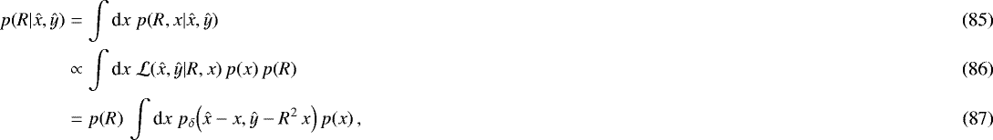 (85) (86) (87)
where  shall be the likelihood of
  given a value pair (x, R), and the product p(x) p(R) is the joint prior of (x, R) (see Gelman et al. 2003, for a introduction to Bayesian statistics). We see that the integral in the last line,
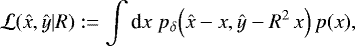 (88)
(88)
has to be the likelihood of  for a given ratio R. We are thus essentially fitting a two-parameter model (R, x) to ŷ = R2 x and
  followed by a marginalising over x. Coming back to our statistical analysis of the aperture statistics, y and x would be here
  and
and  , for example, and
  is the (projected) bias factor b2D. For our full analysis, however, we have to jointly constrain b2D and the correlation factor r2D for a set of aperture radii θi in a more general approach.
To implement a general approach involving nd aperture radii and both the bias and correlation factors for all radii simultaneously, we combine the measurements of aperture moments inside the data vector with the (observed) elements
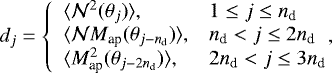 (89)
(89)
and we fit this vector by the parameters m(Θ, x) with template parameters Θ (Table 2) and (theoretical) vector elements
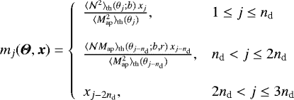 (90)
(90)
using a PDF pδ(δd) that accounts for the correlated noise δd in the aperture statistics. The details of this PDF are given below. We note that the explicit normalisation fb (θi) and fr (θi) disappears here because both the theoretical and observed ratio statistics {(b2D(θi), r2D(θi))} are normalised in exactly the same way. However, the normalisation is indirectly present through the ratio of theoretical aperture moments in m(Θ, x) so that a wrong normalisation will introduce a bias in the reconstruction. Similar to the previous illustration, we integrate over the nuisance parameter 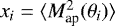 to obtain the marginal likelihood
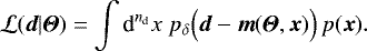 (91)
(91)
We adopt a uniform prior p(x) for x with the additional condition that the variance of the aperture mass has to be positive or zero.
The measurement noise δd in the aperture statistics approximately obeys Gaussian statistics, which are characterised by a noise covariance N =⟨δd δdT⟩; the mean ⟨δd ⟩ vanishes by definition. The exact covariance N, however, is unknown so that we estimate N from the data themselves by  , obtained with njk jackknife realisations of the data (Appendix B). We include the uncertainty of
  in the posterior of the spatial biasing functions by analytically marginalising over its statistical error. As shown in Sellentin & Heavens (2016), this produces for Gaussianδd a multivariate t-distribution for the noisemodel pδ(δd),
 (92)
(92)
where  .
.
To approximately evaluate (91), we perform a numerical Monte Carlo integration
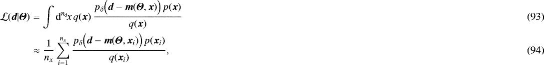 (93) (94)
for which
 (95)
(95)
is a so-called importance function of the Monte Carlo integral, and 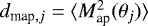 are the measured variances of the aperture mass at θj; the vectors xi ~ q(x) are nx random realisations of the importance function; the matrix
  denotes our estimate for the inverse covariance of noise in dmap, that is that of
  alone, which we also obtain from jackknife samples and the estimator in Hartlap et al. (2007). The purpose of the importance function q(x) is to improve the convergence of the Monte Carlo sum (94) by producing a higher density of sampling points xi where most of the probability mass of pδ(d −m(Θ, x)) is located (e.g. Kilbinger et al. 2010). We note that for any q(x) the sum always converges to the same
  as long as q(x) is proper and q(x) > 0 for all x. To save computation time, we initially prepare nx = 103 realisations xi and reuse these for every new estimation of the marginal likelihood in (94).
We explore the posterior distribution of parameters Θ in the template, that is
 (96)
(96)
by applying sampling with the Multiple-Try Metropolis, where the constant evidence E(d) is not of interest here (Martino & Read 2012). We assume that the prior p(Θ) is uniform on a linear scale for all parameters within their defined boundaries (see Sect. 5.2) and 0 < bls ≤ 3. Different Monte Carlo chains can be combined by joining the different sets of sampling points from independent Monte Carlo runs. If the joint sample is too large to be practical, a resampling can be applied. This means we randomly draw a subset of points Θi from the joint sample. Depending on the details of the adopted Monte Carlo Markov chain (MCMC) algorithm, the probability of drawing Θi in the resampling has to be proportional to its weight, in case points are not equally weighted.
Finally to conclude the reconstruction, we map the Monte Carlo realisations of Θ in the joint sample to a set of spatial biasing functions. The final set then samples the posterior distribution of b(k) and r(k).
6.2 Marginalisation of errors in the galaxy-bias normalisation
For our analysis, the fiducial cosmology and the intrinsic alignment of sources is exactly known by the cosmological model in the mock data. For future applications, however, it may be necessary to additionally marginalise over an a priori uncertainty p(π) of cosmological parameters π for the normalisation of the galaxy bias, meaning that the Θ posterior is
 (97)
(97)
where  is the likelihood of d for a given set Θ and fiducial cosmology π. Numerically the marginalisation over π can be achieved, as indicated by the right-hand side of (97), by (i) randomly drawing a realisation πi from the prior p(π), (ii) by performing the Monte Carlo sampling of the posterior in Eq. (96) for the fixed fiducial cosmology πi ~ p(π), and (iii) by combining the different chains with varying π. Concretely, let us call the resulting Monte Carlo sample from step (ii)
  . We repeat this step nπ times for different cosmologies. For joining the chains in step (iii), we randomly draw one Θi from each sample
  to produce nπ new vectors Θ that go into the final sample. We repeat this random selection of nπ-tupels until the final sample has the desired size. We may apply the same technique to also marginalise over errors in the redshift distributions of lenses and sources, or the uncertainties in the II and GI models.
6.3 Galaxy number density as prior
The halo model provides a prediction of the mean galaxy density  , Eq. (83), that can be included in the template fit to improve the constraints on the otherwise poorly constrained pivotal mass mpiv. We may achieve this by adding the log-normal likelihood
 (98)
(98)
to the logarithm of the marginal likelihood in (94). Here we denote by  the root-mean-square (RMS) error of the logarithmic number density
  estimated from the data.
A reasonable prior on  can also be found if
  is not available as it is assumed here. The number density of galaxies is for redshifts z ≲ 2 typically of the order of 10−2 to 10−1 h3 Mpc−3, or smaller for sub-samples (e.g. Conselice et al. 2016). Therefore in the reconstruction of our biasing functions, we employ a weak Gaussian prior of
 (99)
(99)
for the galaxy number density, and we impose an upper limit of  to prevent a non-physically high number density of galaxies. We found that the upper limit improves the convergence of the MCMCs as chains can get stuck at low values of mpiv with unrealistically high values of
  .
.
7 Results
In the following, we report our results for the reconstructed biasing functions for the galaxy samples SM1 to SM6, RED, and BLUE inside the two redshift bins low-z ( ) and high-z (
 ). We concentrate on the reconstruction accuracy and precision although the template parameters found in the reconstructions are also available in Appendix D. If not stated otherwise, the results are for mock sources with a shape-noise dispersion σϵ = 0.3 and without reduced shear. As an additional test of the methodology, we use generic templates for a non-physical model of the spatial biasing functions and compare the results to those of our physical templates. Furthermore, we estimate the systematic error in the bias normalisation originating from various conceivable sources. The final sub-section is a demonstration of our technique with data from the Garching-Bonn Deep Survey (GaBoDS).
7.1 Reconstruction accuracy and precision
Figures 7 and 8 are a direct comparison of our reconstructed biasing functions for all samples (shaded regions) to the true  and
and  in the three-dimensional simulation cube of the MS shown as red data points; we use the snapshot redshifts
  for low-z and high-z respectively.The shaded regions indicate the 68% and 95% posterior intervals (PI) of our posterior constraints. In order to accommodate many reconstructions, we have shifted the biasing function along the y axes by a constant value that is indicated in the legend of each plot. We note that most functions are shifted downwards so that relative errors might appear larger than in reality. The left panels show b(k), the right panels r(k). Figure 7 displays only reconstructions for the stellar-mass samples where the top row is for the low-z samples and the bottom row for the high-z samples. Similarly, Fig. 8 shows the results for the RED and BLUE samples, now low-z and high-z combined inone figure.
Overall we find a good agreement between a reconstruction and the true biasing functions, although significant disagreements are also visible. Most prominently, we find disagreements at large scales, this means at small wave numbers k ≈ 0.05 h Mpc−1, for the low-z b(k) of RED, SM1, and SM5; or at small scales, k ≈ 10 h−1 Mpc, for the high-z r(z) of SM2 or BLUE; the function low-z b(k) of SM2 and SM3 is a few per cent offset on all scales, which may be an indication of a normalisation error. The disagreement at high k ≳ 10 h−1 Mpc could be related to insufficient sampling by our MCMC because the results improve significantly for samples without shape noise, which reduces the statistical error at θap ≈ 2′ (not shown). It is also possible that the statistical model of the likelihood in Eq. (92) is inaccurate and, as a consequence, underestimates the error distribution in the tail of the posterior at large k.
To quantify the method accuracy, we compare the reconstruction b(k) or r(k) to the true biasing function by the following metrics  and Δf; the subscript “f” is either “b” for b(k) or “r” for r(k). The metrics compare the biasing functions at a discrete set {ki: i = 1…nk} of nk = 10 wave numbers between 0.05 ≤ k ≤ 10 h Mpc−1, which we equally space on a log scale. In the equations, we denote by f(k) the posterior median of either b(k) or r(k) in the reconstruction, and σ2(k) is the variance of the posterior at a given k. In addition, we denote by ftrue(k) the true biasing function and by
  its standard error. The variance
  is indicated by the error bars of the red data points in Figs. 7 and 8; it is usually negligible compared to σ2 (k). Our first metric
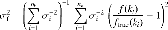 (100)
(100)
then quantifies the average fractional error over the range of k, weighted by the inverse statistical error  . For
. For  , we change the lower limit of k to 0.3 h Mpc−1 to avoid a seemingly too optimistic metric: by definitionr(k) is in the reconstruction close to the true r(k) = 1 of the MS data, which makesσi relatively small and therefore assigns too much weight to k ≲ 0.3 h Mpc−1. The second metric
 (101)
(101)
yields the most significant deviation in units of σi; it is a measure for the strongest outlier within the k-range.
Table 3 lists σf (in %) and Δf for all galaxy samples and redshift bins; the last rows are averages and dispersions for each table column. The table consists of two blocks of which we summarise the left-hand columns, “physical”, here, and the right-hand column, “generic”, in Sect. 7.2 hereafter. The values for σb are typically in the range 5.4 ± 2.9% for low-z samples and slightly better with 3.6 ± 1.7% for the high-z samples. The accuracy of σr is consistently 3.0 ± 2.0% for both redshift bins. For the outlier statistics, we find on average Δb = 2.2 ± 1.2σ and Δr = 2.2 ± 1.8σ for all redshifts, which, however, can attain high values of 6 − 7σ in a few cases, high-z BLUE and SM2 for instance. We find these high values to be associated with mismatches of r(k) at k ≈ 10 h Mpc−1. This corresponds to θap ≈ 1′, thus to the lower limit of the angular scales that we sample in the mock analysis (cf. bottom and top x-axis in Fig. 6).
Moreover, we quantify the statistical precision of our reconstruction at wave number ki by the ratio of σ(ki) and the median of the posterior of either f(ki). For an average over all galaxy samples and the reconstruction within the range 0.05 ≤ k ≤ 10 h Mpc−1, we find a precision of 6.5 ± 2.1% for b(k) and 5.5 ± 5.7% for r(k); we combine the low-z and high-z samples because the precision is very similar for both bins. The errors denote the RMS variance of the precision.
In summary, we find that a method accuracy of around 5% with most significant deviations at scales of k ≳ 10 h Mpc−1 which, however, are not supported by the measurements and have to be extrapolated by the templates. The statistical precision of the reconstructions is typically between 5–10% for our fiducial survey and lens samples.
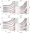 |
Fig. 7 Biasing functions b(k) (left panels) and r(k) (right panels) for all mock galaxy samples SM1 to SM6 and two redshift bins. The top figure is for the low-z samples ( |


Overview of the reconstruction accuracy by listing the mean fractional errors σb,r and extreme outliers Δb,r of the inferred biasing functions b(k) and r(k), respectively, in %.
7.2 De-projection with generic templates
We repeat the reconstruction of b(k) and r(k) for our mock data with the Padé approximants
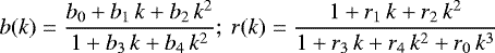 (102)
(102)
as generic templates of the biasing functions in Sect. 6.1 (without an  regularisation). The bi and ri denote ten coefficients, which we restrict to |bi|, |ri|≤ 100 in the fit. These generic model templates are related to the fitting function for b2 (k) in Cole et al. (2005). We found that the Padé approximants are very good descriptions of the red data points in Figs. 7 and 8. By fitting generic templates we therefore investigate whether the foregoing inaccuracies in the reconstruction with the physical templates might be related to a model bias. If this is the case, we should obtain a better reconstruction here. We note that the particular approximant of r(k) asserts r → 1 for k → 0, and that in the generic templates, unlike the physical templates, b(k) is independent from r(k).
Compared to the halo model, the generic templates produce a similar (low-z) or somewhat worse (high-z) reconstruction but are prone to more extreme deviations from the true biasing functions. The right-hand block of values (“generic” in Table 3) summarises the metrics of the reconstructions with the generic templates and compares them to the metrics with the physical templates (“physical” on the left-hand side). We find an increased inaccuracy for the high-z samples, especially for SM5, SM6, and RED; in particular the reconstruction of low-z RED has not improved here. The worse reconstruction for high-z is because of the inability of the generic templates to extrapolate to small spatial scales which is more important for high-z where the same angular range corresponds to larger spatial scales. In a few cases, the generic templates produce very significant deviations, mostly on small scales and indicated by Δb,r, which are absent in the physical templates.
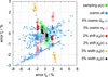 |
Fig. 9 Average error in the galaxy-bias normalisation fb (x-axis) and fr (y-axis). The points show as indistinguishable the errors of all galaxy samples SM1-4, BLUE, and RED together; the point styles indicate the redshift bin and what is varied. Symbols as in the figure key indicate the low-z samples, inverted symbols indicate the high-z samples (e.g. solid and open circles). The “cosmo” and “sampling p(z)” data points reuse the same galaxy samples many times with random normalisation errors. The solid line marks the estimated error for high-z samples dueto the baryon uncertainty. The fiducial cosmology is WMAP9. See text for more details. |
7.3 Errors in the galaxy-bias normalisation
The ratio statistics are normalised with respect to unbiased galaxies in a fiducial model. Systematic errors in the normalisation affect the amplitude of the de-projected biasing functions. Therefore, we explore the robustness of the overall amplitude of b(k) and r(k) with respectto changes in the fiducial cosmology and the adopted redshift distributions in the normalisation (see Eqs. (16) and (17) that are evaluated for the unbiased galaxies). We note that fb and fr normally show little dependence on θap so that changes in the fiducial model mainly scale the projected biasing functions up or down.
The functions fb(θap) and fr(θap) will be the correct normalisation of the galaxy bias. For Fig. 9, we then compute  (and
(and  ) for variations in the normalisation parameters, and we compute the quadratic mean of relative errors
  over the angular range 1′ ≤ θap ≤ 140′. The data points inside the figure indicate these means
  (x-axis) and
  (y-axis) for particular lens samples. To have a good representation of the scatter between possible lens-galaxy samples, we show results for all galaxy samples SM1-SM6, RED, and BLUE in the same redshift bin together by the same point style if they are subject to the same parameter variation. We give the normalisation errors a plus sign if the average of δb (θap) is positive, and a negative sign otherwise. This flags b(k) (or r(k)) that are overall too high (positive) or too low (negative). We apply variations relative to a default model which has WMAP9+eCMB+BAO+H0 cosmological parameters (Hinshaw et al. 2013); redshift distributions as shown in Fig. 1; a non-linear matter power spectrum according to Takahashi et al. (2012). Inside the plot, data points have the styles shown in the figure key for low-z samples and an inverted point style for high-z samples, such as solid circles (low-z) and open circles (high-z). We vary the following parameters in the default model to quantify their impact on the normalisation.
-
The data points “cosmo all” randomly draw combinations of cosmological parameters from an error distribution centred on the fiducial model
 (103)
(103)In this distribution, errors are uncorrelated and Gaussian with a dispersion of
 (104)
(104)relative to the fiducial π. The exception is Ωλ which we setto Ωλ = 1 −Ωm in all realisations (a fixed K = 0 geometry). These errors are on the optimistic side but consistent with constraints from combined cosmological probes. In addition for each set of parameters, we plot data points for three different transfer functions of Pm(k;χ): Bardeen et al. (1986), and Eisenstein & Hu (1998) with and without baryonic acoustic oscillations (BAOs). These are combined with two different Halofit models of the non-linear power spectrum: Smith et al. (2003) and the more accurate Takahashi et al. (2012). By these variations we mean to broadly account for model uncertainties in the non-linear power spectrum, which produces extra scatter in the plot. In particular, the 10–20% difference between the two versions of Halofit in the regime k ≳ 1 h Mpc−1 accounts to some extent for the theoretical uncertainty of baryons on the small-scale power spectrum (e.g. Springel et al. 2018; Foreman et al. 2016; Harnois-Déraps et al. 2015; Semboloni et al. 2011). We find that errors in the cosmological parameters or the non-linear power spectrum mainly affect the normalisation of b(k), which can be off by about 3.0% (68% confidence level, CL hereafter). The error in r(k) is within 1.1% (68% CL) for high-z or smaller 0.4% (68% CL) for the low-z samples (solid symbols). The straight line inside the figure indicates the locus of errors for the high-z samples that are produced by the baryon uncertainty in the non-linear power spectrum.
For “cosmo Ωm”, we only vary Ωm in the cosmological parameters with the foregoing dispersion. This results in a distribution of data points that is very similar to “cosmo all”. For comparison, “cosmo σ8” varies only σ8. The scatter is now restricted to a small region. Therefore, the normalisation error owing to cosmological parameters is mainly explained by the variations in Ωm.
-
For the data points “sampling p(z)”, we add random shot noise to the redshift distributions. The idea here is that redshift distributions are estimated from a sub-sample of galaxies, which gives rise to sampling noise in the estimated distributions used for normalisation (see e.g. Hildebrandt et al. 2017 who use a weighted sample of spectroscopic redshifts to model the redshift PDF of the full galaxy sample). To emulate the sampling shot noise, we randomly draw n redshifts z ~ p(z) from the true p(z) to build a finely binned histogram of a noisy redshift distribution (Δz = 0.015). We then employ this histogram for
 and
and  . As fiducial values for our 1024 deg2 survey, we adopt n = 104 for the lenses and n = 105 for the sources. These fiducial values imply that we estimate p(z) from spectroscopic redshifts of ~0.5% of the sources and roughly 1%, 2%, 20%, 1% of the lenses in the samples SM1, SM4, SM6, RED/BLUE, respectively. The result is a similar scatter for the low-z and the high-z samples in Fig.1. The error is typically within 0.5% for b(k) and r(k) (68% CL).
 -
The datapoints “shift pd(z)” vary the mean in the lens redshift distribution. For this, we systematically shift z↦z (1 + δz) by δz = ±2%, which is twice as large as the typical error on the mean redshift reported in Hildebrandt et al. (2017). The impact differs for the low-z (solid circles) and the high-z samples (open circles). For systematically higher redshifts in low-z, this means δz > 0, b(k) is too large and r(k) is too low. For high-z and δz > 0, we find that both b(k) and r(k) are too high in amplitude. For δz < 0, the effects are exactly reversed. The overall systematic normalisation error is nevertheless not greater than typically 2% for b(k) and 1−2% for r(k).
-
The datapoints “width pd(z)” vary the width of the lens redshift distribution. This we emulate by mapping
 to a new PDF that is then used for the normalisation. For a Gaussian density pd(z), this maps the dispersion to σ↦σ (1 − δσ) while leaving the mean and Gaussian shape in the new PDF unchanged. For skewed distributions, δσ≠0 also moves the mean of the PDF. To account for this unwanted (small) side effect, we shift every PDF to assure that it retains its original mean redshift. We consider δσ = ±5% here. The effect of squeezing, this means δσ > 0, is similar for low-z and high-z: b(k) is too low, r(k) is too high, with errors of around 2 − 3% for b(k) and r(k). A stretching, δσ < 0, has the reverse effect on both redshift bins.
 -
The data points “shift ps(z)” and “width ps(z)” explore the effect of errors in the mean or width of the source ps(z). Shifting by δz = +2% produces too high b(k) for low-z and high-z (1.9%), too high r(k) for low-z (0.5%), and a too low r(k) for high-z (1.0%). The reverse behaviour is present for systematically lower redshifts with δz = −2%. Changes in the width of the distribution with δσ = ±5% have a 0.5% effect for b(k) and r(k), with low-z samples being slightly less affected: a systematically wider distribution gives a too low b(k) and a too high r(k); the reverse effects apply for systematically narrower distributions, that is for δσ > 0.
-
The intrinsic alignment of sources contributes to both
 and
and  and thereby can have an impact on b2D
and r2D. We account for this in the normalisation by II and GI models (see Sect. 3.3). If unaccounted for, as assumed here, we bias b2D
by the error in
and thereby can have an impact on b2D
and r2D. We account for this in the normalisation by II and GI models (see Sect. 3.3). If unaccounted for, as assumed here, we bias b2D
by the error in  that is used in the normalisation fb, Eq. (16). This error is plotted in Fig. 10 for varying values of
Aia
and angular scales θap. The normalisation error in r2D
is determined by the error in
that is used in the normalisation fb, Eq. (16). This error is plotted in Fig. 10 for varying values of
Aia
and angular scales θap. The normalisation error in r2D
is determined by the error in  used for fr, Eq. (17), which is plotted in Fig. 11 for SM4 high-z
as an example; the errors of other high-z
samples are comparable. For the low-z
samples, the overlap of lens and source redshifts is small so that the error in
used for fr, Eq. (17), which is plotted in Fig. 11 for SM4 high-z
as an example; the errors of other high-z
samples are comparable. For the low-z
samples, the overlap of lens and source redshifts is small so that the error in  is negligible compared to the error in
  . Therefore, the normalisation error for r2D
in low-z
samples is approximately that of b2D
in Fig. 10. For |Aia|≲ 2, the normalisation error of b2D
and r2D
is typically within ± 5% at scales θap ≳ 1′.
. Therefore, the normalisation error for r2D
in low-z
samples is approximately that of b2D
in Fig. 10. For |Aia|≲ 2, the normalisation error of b2D
and r2D
is typically within ± 5% at scales θap ≳ 1′.
A summary of normalisation errors and their estimated magnitude is listed in Table 4. We find that the response to errors in the redshift distributions is approximately linear for δz and δσ that are within several % so that the quoted values could be scaled.
Summary of possible systematic errors and their expected impact on the reconstruction of b(k) or r(k) for a WMAP9 cosmology and our galaxy samples.
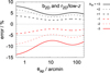 |
Fig. 10 Systematic relative errors in b2D(θap) (low-z and high-z) and r2D(θap) (only low-z) when II andGI terms are ignored in the normalisation of the galaxy bias. Different lines show predictions for different values of Aia with sourcesas in our mock survey. The fiducial cosmology is WMAP9. |
7.4 Shear bias and reduced shear
As another source of systematic error, we consider a residual bias in the shear estimators that has not been properly corrected for in the lensing pipeline. Following (Kitching et al. 2012; K+12 hereafter), we quantify a shear bias by ⟨γ⟩ = (1 + m) γ + c for average estimated shear ⟨γ⟩ in an ensemble of sources that are subject to the same γ: m is the so-called multiplicative bias and c is the additive bias. For a crude estimate of the impact of m on the measurement of b2D(θap) and r2D(θap), we assume a constant and real-valued m. A value of m≠0 produces a bias of 1 + m in the measured aperture statistics  and
and  . Therefore, applying our methodology while ignoring m will scale the amplitude of b(k), Eq. (14), by
  but it will not change r(k) in Eq. (15). Contemporary lensing techniques reach a typical accuracy of |m|≈ 1%, therefore we expect a similarly small systematic error for b(k) (K+12).
A residual additive bias c does not affect the aperture statistics if it is constant. If, on the other hand, c varies at a scale within the sensitiveℓ-range of the aperture filter, we could have significant contributions to the measured  , depending on the power of the c-fluctuations. Our polynomial filter in Eq. (12) has its maximum sensitivity for the angular wave number
  or angular scale θc = 2π∕ℓc ≈ 1.44 θap (van Waerbeke 1998). The typical residual amplitudes of c after a calibration correction of ξ± are of the order of 10−5 (K+12; Appendix D4 in Hildebrandt et al. 2017) so that systematic errors owing to c fluctuations are probably below one % for
  , which is the case for θap ≲ 2 deg and typical sources with zs ≈ 1 (see the data points in Fig. 2). The statistic
  is not affected by the additive shear bias in the likely absence of correlations between lens positions and fluctuations of c, or is presumably corrected for by subtracting the correlation between random lens positions and shear in the data (see the estimator in Eq. B.3).
With regard to reduced shear, our analysis assumes that the ϵi are estimates of shear γ(θi), whereas they are in reality estimates of the reduced shear gi = γi∕(1 − κi). While ⟨ϵi⟩ = γi is a good approximation for weak gravitational lensing and substantially simplifies the formalism in Sect. 3, we will have some systematic error. To quantify this error, we redo the reconstruction of the biasing functions for a new shear catalogue where the intrinsic source ellipticities are sheared by gi rather than γi; source positions and intrinsic shapes do not match between the old and new catalogues. For the new catalogues, we obtain a set of values  , Eq. (100), which we statistically compare to the previous values σf in Table 3 by fitting an average parameter δred for the relative difference, defined by
  , to all samples and redshift bins. For all values of σb and σr combined, we find no significant differences between the new and old shear catalogues, which means δred is consistent with zero; the upper limit is δred ≲ 13% (68% CL). For an average of ⟨σf ⟩ = 3.8%, the additional inaccuracy due to reduced shear is therefore less than 13% ×⟨σf⟩≈ 0.5%.
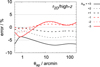 |
Fig. 11 As in Fig. 10 but now for r2D(θap) high-z. Shown are results from SM4 but the values are similar for the other samples. |
7.5 Garching-Bonn Deep Survey
Finally, we apply our procedure in a first demonstration to data in the GaBoDS (Simon et al. 2007, SHS07 hereafter; Hetterscheidt et al. 2007). Because of its comparatively small effective survey area of roughly 15 square degree, the statistical power of GaBoDS is no longer competitive to measurements in contemporary surveys. Nevertheless, the results presented here shed some new light on the nature of the lens galaxies in SHS07 and round off the past GaBoDS analysis. We plan to apply our methodology to more recent lensing data in an upcoming paper.
As lens sample in GaBoDS we choose FORE-I galaxies, which comprise R ≤ 21.0 flux-limited galaxies with mean redshift  ; the RMS dispersion of the lens redshifts is 0.16. The source galaxies are flux-selected between 21.5 ≤ R ≤ 24.0 and have
  (see Fig. 3 in SHS07 for the redshift distributions of lenses and sources in these samples). For the estimators, we bin the two-point correlation functions (B.2)–(B.4) between 7 arcsec and 46 arcmin using 4100 linear bins and merge the catalogues of the npatch = 52 GaBoDS fields also used in SHS07. In contrast to SHS07, we only use six aperture scales between 2 and 23 arcmin, equidistant on a logarithmic scale, because of the strong correlation of errors between similar aperture scales. The correlation matrix of statistical (jackknife) errors can be found in Fig. 12. Furthermore, we normalise the new measurements by a WMAP9 cosmology, Eq. (103). In contrast to the foregoing analyses with our mock MS data, for which we measure the aperture statistics up to degree scales, we here have to use Eq. (69) to extrapolate the large-scale bias bls, which is then no longer a free parameter. For the halo bias factor bh(m), needed in this extrapolation, we employ the fitting formula in Tinker et al. (2005). Owing to the lack of information on an intrinsic alignment of GaBoDS sources, we do assume Aia = 0. A value of |Aia|≲ 2 could therefore shift the amplitude of b2D by up to 10% to 15%, mainly because of the GI term, and that of r2D by up to 2%.
Our updated measurements are shown in the left panel of Fig. 13 as b2D and r2D by the black data points designated in SHS+07. To obtain these points from the observed aperture-moment statistics, we randomly draw realisations of the aperture statistics from a Gaussian likelihood based on our jackknife data covariance. The open squares show the median and 68 percentiles of the normalised bias parameters from this Monte Carlo process, computed with Eqs. (14) and (15) for each realisation; the open circles are the mean of the realisations, which are different to the median owing to the skewness in the error distribution. The shaded regions indicate the 68% and 95% PI of the posterior (projected) biasing functions. The red stars are measurements with VIRMOS-DESCART data, broadly consistent with ours, for flux-limited galaxies with a similar selection function (Hoekstra et al. 2002).
The right panel of Fig. 13 depicts the posterior of the template parameters that provide a physical interpretation of the galaxy bias. We take from here that the scale dependence of the galaxy bias mainly originates in a scale dependence of b(m): between halo masses of 1013 to 1014 h−1 M⊙ there is a relative scarcity of galaxies, which is qualitatively comparable to the BLUE low-z sample (see Fig. D.1). The HOD variance is consistent with a Poisson model, that means V (m) = 0, albeit only weakly constrained. The 68% PI of the pivotal halo mass is mpiv = 1011.48+0.72−0.81 h−1 M⊙, and the fraction fcen = 0.50 ± 0.31 of halos open for central galaxies is essentially the uniform prior, which has the variance  and the mean 0.5. The posterior galaxy number density is
  .
.
Figure 14 displays the posterior distribution of the de-projected biasing functions and the 68% PI for FORE-I galaxies. The biasing functions are an average for the redshift range covered by the lens galaxies. The GaBoDS data probe primarily the one-halo regime θap ≲ 20 arcmin; the large-scale bias of  visible at k ≪ 1 h Mpc−1 is extrapolated. The red data points show the biasing functions of BLUE low-z for a qualitative comparison.
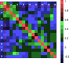 |
Fig. 12 Correlation matrix Cij of measurement errors for three kinds of aperture statistics of FORE-I lenses in the GaBoDS analysis. The integers on the two axes inside the matrix refer to either the i or j index. Values 1 ≤ k ≤ 6 for k being either i or j refer to errors of |

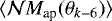

8 Discussion
In this study, we have outlined and successfully tested a refined technique to measure in contemporary lensing surveys the scale-dependent galaxy bias down to non-linear scales of k ~ 10 h−1 Mpc for lens galaxies at z ≲ 0.6. To test our reconstruction technique, we employ a fiducial survey with a sky coverage of ~ 1000 deg2, and a photometry and a survey depth as in CFHTLenS. To construct realistic samples of lenses and sources, we have prepared mock catalogues that are consistent with those used in SES13 and Saghiha et al. (2017). Despite some variations in survey depth and area, these survey parameters are similar to the ongoing Kilo-Degree Survey (KiDS), Dark Energy Survey (DES), or the survey with the Hyper Suprime-Cam (Kuijken et al. 2015; Becker et al. 2016; Aihara et al. 2018). If the galaxy-bias normalisation is perfect, our technique applied to these data can achieve a statistical precision within the range of 5–10% (68% CL), if similar lens and source samples are targeted, and a slightly better accuracy of 3−7% (68% CL; see Table 3). For the high-z samples, the accuracy will be somewhat higher with 3−5%. On the other hand, it is clear from our overview Table 4 that the accuracy of the galaxy-bias normalisation is in fact limited, mainly by our knowledge of the intrinsic alignment of sources, cosmological parameters, and the galaxy redshift distributions. With a broad knowledge of |Aia|≲ 2 and the specifications for the normalisation errors in Table 4, we conclude that systematic errors would potentially degrade the overall accuracy to approximately 15% for b(k) and 10% for r(k). For fully controlled intrinsic alignment of sources, these errors could be reduced by 5%. An additional reduction by 3% may be possible by controlling the redshift distributions (their mean and variance) in the normalisation to 1% accuracy. For the fiducial cosmology, the knowledge of Ωm is of most importance while the normalisation of the ratio statistics is less affected by σ8.
For a future method improvement, various problems could be of interest: (i) approximations in the formalism or estimators of Sect. 3; (ii) an inaccurate statistical model for the likelihood function; (iii) a model bias in the templates. We discuss a few problems in the following. With regard to our statistical model, we find indeed evidence for deviations from a Gaussian model of the joint aperture statistics (see Appendix C); a Gaussian model is explicitly assumed in Eq. (91). However, the magnitude of a bias owing to a Gaussian model is not clear and requires more research. For example, deviations from a Gaussian distribution in broadly related cosmological analyses with the aperture mass Map are reported in Simon et al. (2015) and Hartlap et al. (2009) where non-Gaussian corrections to the likelihood produce insignificant changes in one case but not in the other. Interestingly for our data, the most inaccurate reconstruction (for small k) is that of RED low-z, which shows a strong indication of a non-Gaussian error distribution for  at large angular scales (see Table B.1). Moreover, our likelihood model employs an error covariance that we estimate by the jackknife technique. The jackknife technique is known to underestimate cosmic variance, in particular for angular scales comparable to the size of sub-fields used for the jackknife sample (Friedrich et al. 2016). However, this problem is partly addressed inour analysis by using ratio statistics, which is less affected by cosmic variance (Bernstein & Cai 2011). While this may not be sufficient for future surveys, it seems to be so for contemporary surveys because cosmic variance is included in our assessment of the reconstruction accuracy. Finally, a model bias in our templates for b(k) and r(k) is arguably unlikely, at least for our simulated galaxy samples, because the purely generic models in Eq. (102) do not produce a more accurate reconstruction of the biasing functions although they are excellent fits to the true biasing functions (see Table 3). Nevertheless, a relevant model bias could arise through our assumption of a non-evolving galaxy bias for galaxy samples with a distance distribution that is broad compared to the galaxy-bias evolution.
Our physical templates for the biasing functions b(k) and r(k) are also insightful for a basic physical interpretation of the scale dependence of galaxy bias. On the one hand, the physical parameters in the physical templates describe the HOD of the actual galaxy population. On the other hand, these HOD parameters have only a moderate accuracy because our relatively simple halo model lacks the implementation of recently identified effects such as halo exclusion, non-linear or stochastic halo clustering, assembly bias, galaxy conformity, or a scale-dependent halo-bias function (Baldauf et al. 2013; Gao & White 2007; Kauffmann et al. 2013; Tinker et al. 2005). And our model has a comparably simplistic treatment of central galaxies. According to Cacciato et al. (2012), by taking ratios of the aperture statistics we are, however, probably less sensitive to these shortfalls in the halo model. We therefore expect the HOD parameters in our templates not to be more accurate than 10–20% compared to the true HOD in the lens sample, based on the reported biases in the cited literature. We stress that this does not necessarily pose a problem for the de-projection as long as the templates are good fits to the true biasing functions. With regard to a basic interpretation of galaxy bias, we nevertheless take from the discussion in Sect. 5.3 that central galaxies and a non-Poisson HOD variance produce a scale-dependent bias most prominently towards small scales, namely in the regime that is dominated by low-occupancy halos with m ≲ mpiv. A strong scale dependence over a wider range of spatial or angular scales and a non-monotonic behaviour may be produced by a mean biasing function b(m) that varies with halo mass m; in particular only b(m) affects the large-scale bias. Interestingly here, the effect of central galaxies is different from that of a non-Poisson variance: central galaxies increase both b(k) and r(k) for larger k, whereas a non-Poisson variance induces opposite trends for b(k) and r(k). Therefore, the measurement of biasing functions can in principle constrain both b(m) and the excess variance V (m) to test galaxy models, although predictably with limited accuracy in contemporary surveys (see Fig. D.2).
A demonstration of our reconstruction technique to data in the GaBoDS suggests that the R ≤ 21 flux-limited sample of lens galaxies FORE-I consists mainly of blue galaxies in the field. Figure 14 reports our reconstruction of the biasing functions for the FORE-I sample in Simon et al. (2007). The physical parameters in the right panel of Fig. 13 show that these galaxies tend to avoid halos in the broad mass range 1013–1014 h−1 M⊙ and thereby produce the relatively low (mean) values of b2D ≈ 0.8 and r2D ≈ 0.6 and their scale dependence between a few and 20 arcmin (left panel; see also the measurements by H+02 for similar lens galaxies with comparable results). Consequently, they are presumably in majority field and group galaxies. The reconstructed biasing functions also broadly match those of BLUE low-z, which supports this interpretation. Clearly, the BLUE low-z sample does not have the same selection function as FORE-I so that this comparison is certainly only qualitative. For a quantitative test of galaxy models with more recent galaxy surveys, simulated and observed galaxies have to be carefully selected to obtain consistent samples. If this succeeds, both our little demonstration with the 15 deg2 GaBoDS data and the multiplicity of biasing functions visible in Figs. 7 and 8 promise useful constraints for galaxy models.
 |
Fig. 13 Left:posterior model of r2D(θap) (top) and b2D(θap) (bottom) based on the GaBoDS measurements FORE-I (shaded regions with 68% and 95% PI). Shown as black open squares are the median values and a 68% interval around the median for the measured b2D and r2D; the open circles indicate the mean. The red-star data points H+02 show the measurements by Hoekstra et al. (2002) for comparison. Right: 68% PI posterior of the excess HOD variance V (m) with open box for the mass scale of the pivotal mass mpiv (top); 68% PI posterior of the mean biasing function b(m) and fcen as open triangle (bottom). The fiducial model has WMAP9 parameters. |
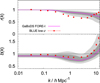 |
Fig. 14 Reconstructed biasing functions of FORE-I galaxies in GaBoDS. Shown are the 68% and 95% PI of b(k) in the bottom panel and that of r(k) in the top panel. The biasing function are an average over the redshift range 0.34 ±0.16 for a WMAP9 cosmology. The red data points show the biasing function of BLUE low-z, which have asimilar b(m). |
Acknowledgements
We thank Hananeh Saghiha for preparing the RED and BLUE galaxy samples. We also thank Catherine Heymans and Indiarose Friswell for comments on the shear bias, and Peter Schneider for general comments on the paper. This work has been supported by Collaborative Research Center TR33 “The Dark Universe” and by the Deutsche Forschungsgemeinschaft through the project SI 1769/1-1. Patrick Simon also acknowledges support from the GermanFederal Ministry for Economic Affairs and Energy (BMWi) provided via DLR under project no. 50QE1103 –and expresses his deep gratitude towards his curiosity-inspiring Opa Siegfried Kamradt. Stefan Hilbert acknowledges support by the DFG cluster of excellence “Origin and Structure of the Universe” (www.universe-cluster.de).
Appendix A Impact of shot-noise subtraction on real-space biasing functions
Let the functions ξg(x) = ⟨δg(0)δg(x)⟩, ξmg(x) = ⟨δg(0)δm(x)⟩, and ξm (x) = ⟨δm(0)δm(x)⟩ be the correlation between density contrasts of galaxies and matter at lag x, and
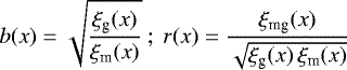 (A.1)
(A.1)
the biasing functions in real space. We show for two specific scenarios of the toy model in Sect. 4.3 that the subtraction of Poisson-shot noise can produce r(x) > 1 for x > 0. To this end, we first work out the real-space biasing functions b(x) and r(x) for the toy model. The correlation function ξ(x) for a given power spectrum P(k) is
:= \frac{1}{2\pi^2x}\int_0^{\infty}{\textrm{d}} k\;k\,P(k)\,\sin{(k\,x)}, \end{equation*}](/articles/aa/full_html/2018/05/aa32248-17/aa32248-17-eq241.png) (A.2)
(A.2)
where we have defined the integral operator [P](x) on the function P(k). For our toy model, we hence find ξg(x) = [Pg](x), ξgm(x) = [Pgm](x), and ξm (x) = [Pm](x) with the one-halo terms Eqs. (46)–(48) and n(m) ∝ δD(m − m0). We assume x > 0 in the following. After some algebra, we find
} {[\tilde{u}_{\textrm{m}}^2](x)}\,\frac{1}{r(x)}; \\ r(x)&=& \frac{[\tilde{u}_{\textrm{m}}\cdot\tilde{u}^q_{\textrm{g}}](x)} {\sqrt{[\tilde{u}_{\textrm{g}}^{2p}](x)\,[\tilde{u}_{\textrm{m}}^2](x)}}\, \left(1+\frac{{\mathrm{\Delta}}\sigma_N^2(m_0)}{\langle {N|m_0} \rangle}\right)^{-1/2}\!\!\!, \end{eqnarray}](/articles/aa/full_html/2018/05/aa32248-17/aa32248-17-eq242.png) (A.3) (A.4)
(A.3) (A.4)
where $](/articles/aa/full_html/2018/05/aa32248-17/aa32248-17-eq243.png) denotes the Fourier back-transform of the product
denotes the Fourier back-transform of the product  ; it is hence the convolution of f(x) and g(x). These equations assume um(x) ≥ 0 for all lags x such that the convolution
 =[\tilde{u}_{\textrm{m}}\cdot\tilde{u}_{\textrm{m}}](x)$](/articles/aa/full_html/2018/05/aa32248-17/aa32248-17-eq245.png) is positive definite as well. Now, for faithful galaxies we have ũm(k, m0) = ũg(k, m0) and p = q = 1, and therefore analogous to (b(k), r(k))
is positive definite as well. Now, for faithful galaxies we have ũm(k, m0) = ũg(k, m0) and p = q = 1, and therefore analogous to (b(k), r(k))
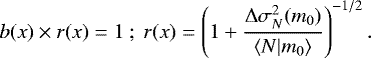 (A.5)
(A.5)
Clearly, we find r(x) > 1 for a sub-Poisson HOD variance also for real-space biasing functions. Moreover, for galaxies with ũm(k, m0) = ũg(k, m0), Poisson HOD variance ( ), and central galaxies in low-occupancy halos (p = 1∕2, q = 0), we arrive at
}{[\tilde{u}_{\textrm{m}}^2](x)}}. \end{equation*}](/articles/aa/full_html/2018/05/aa32248-17/aa32248-17-eq248.png) (A.6)
(A.6)
Therefore, also here we find r(x) > 1 for at least some lags x because the convolution of um(x) with itself has to be <u_{\textrm{m}}(x)$](/articles/aa/full_html/2018/05/aa32248-17/aa32248-17-eq249.png) for some x.
for some x.
Appendix B Estimators of aperture statistics
The aperture statistics can be obtained from three kinds of two-point correlation functions based on the positions  of nd lens galaxies on the sky and the positions
  , shear estimators ϵi, and statistical weights wi of ns source galaxies. We estimate these correlation functions as follows.
First, we estimate the shear-shear correlation functions ξ± (ϑ) = ⟨γt(θ + ϑ)γt(θ)⟩±⟨γ×(θ + ϑ)γ×(θ)⟩ for a separation ϑ of two sources, where the tangential, γt, and cross components, γ×, of γ at the source positions are defined relative to the vector ϑ connecting a source pair through γt + i γ× = −ϑ*∕ϑ γ; position or separation vectors use the usual complex-valued notation in a local Cartesian frame on the sky (Bartelmann & Schneider 2001). We define for all estimators a galaxy pair ij with positions  and
and  to be within the separation bin
  if
if 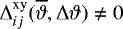 for
for
 (B.1)
(B.1)
Then we estimate the average ξ±(ϑ) for source pairs within the bin  by
by
 (B.2)
(B.2)
where ϵt,i and ϵt,j refer to thetangential components of the shear estimator of the ith or jth source in the pair ij relative to  , and likewise for ϵ×,i and ϵ×,j (Schneider et al. 2002).
Second, we estimate the mean tangential shear  of sources atseparation ϑ from lenses located at θd by
 (B.3)
(B.3)
where now ϵt,j is the tangential component of ϵj relative to  , and
, and  is the first term on the right-hand side of (B.3) for a large sample of random lens positions (Singh et al. 2016).
Third, for the correlation function ωω(ϑ) = ⟨κg(θ + ϑ)κg(θ)⟩ of the lens clustering on the sky, we employ the estimator in Landy & Szalay (1993),
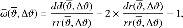 (B.4)
(B.4)
where dd is the normalised number of lens pairs in the separation bin, rr the normalised number of pairs with random positions  out of nr ≫ nd in total, anddr is the normalised number of lens-random pairs:
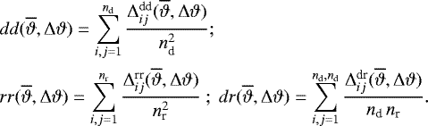 (B.5)
(B.5)
To combine the estimates from npatch different patches, we merge their lens and source catalogues with constant position offsets for each patch such that we never have pairs of galaxies from different patches inside a separation bin. The probability of finding a random-lens position inside a particular patch in the merged catalogue is proportional to the effective, unmasked area of the patch, which is always 16 deg2 for the mock data. For the analysis of the 64 patches mock data, we use as angular binning 5000 linear bins between 1.4 arcsec and 5.7 deg.
Results of KS-test for Gaussianity for three kinds of the aperture statistic at scales θ = 2, 20, 60, 120 arcmin (in this order).
We transform the estimates of the three two-point correlation functions into estimates of the aperture statistics for several θap ∈ [1′, 140′] by a numerical integration of the following equations
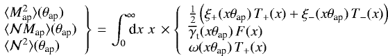 (B.6)
(B.6)
based on the auxiliary functions
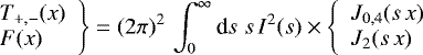 (B.7)
(B.7)
with analytic expressions for T±(x) and F(x) as in Simon et al. (2007). Because of the lower cutoff at 1.4 arcsec in the correlation functions (we set them zero here), we cannot use values of the aperture statistics below around two arcmin where the transformation bias grows to about 10% (Kilbinger et al. 2006). To estimate the statistical errors or covariances between the three aperture statistics and angular scales θap, we employ the jackknife technique with npatch sub-samples that we obtain by removing one patch at a time from the merged catalogue (Friedrich et al. 2016).
In Fig. 2, we plot estimates of  in our mock data as points with statistical errors obtained with the jackknife technique (inflated by a factor of five). The three different styles of the data points are for: (i) shear with shape noise of sources (solid squares); (ii) reduced shear with shape noise (open circles); and (iii) shear without shape noise (solid triangles). The data points are a very good match to a theoretical model GG for the MS cosmology (blue solid line), and they are consistent with each other at the same θap. The statistical errors of data without shape noise are similar to those for sources with shape noise for θap ≳ 10′, which indicates that cosmic variance dominates in this regime for our fiducial survey.
Appendix C Non-Gaussianity of measurement errors
In this appendix, we test for a non-Gaussian distribution of statistical errors in the aperture statistics  ,
,  , and
, and  with a one-dimensional Kolmogorov-Smirnov (KS) test. We perform the KS tests separately for each aperture statistics, denoted by x in the following, and the aperture scales θap ∈{2′, 20′, 60′, 120′}. Since we have only one simulated lensing survey with 1024 deg2 of data, we split the data into independent patches and test the empirical distributions of measurements xi in n = 64 patches of area 4 × 4 deg2 each. We standardise the measurements by computing
  , where
  and σx are the mean and standard deviation, respectively, of the sample {xi: i = 1…n}. For the KS test, we then compare the distribution
  in the mock data to the average distribution F(z) of n normally distributed measurements using the test statistic
  ; here we define the function I(z) = 1 for z ≤ 0 and I(z) = 0 otherwise.
The resulting p-values of our Dn are listed in Table B.1; p-values smaller than 0.05 indicate a conflict with a Gaussian distribution (95% CL). We perform the test for each galaxy sample and redshift bin. For every galaxy sample, we make new realisations of the source catalogues by randomly changing the source positions in the patch and the intrinsic shapes. This explains the differences in the test results for  at identical angular scales. While we expect some failures of the KS test by chance, tensions are clearly visible for
  at θap ≳ 60′ and for
  of the strongly clustered sample RED low-z.
In summary, for  and
and  a Gaussian likelihood of errors is a fair approximation, whereas for
  and around degree scales or more, non-Gaussian features in the error distribution, mainly cosmic variance, are detectable. We note that evidence for non-Gaussian distributions does not necessarily mean that a Gaussian likelihood is an insufficient approximation for a shear analysis.
Appendix D Template parameters of reconstructed biasing functions
Table D.1, and Figs. D.2 and D.1 summarise the posterior distribution of template parameters that are the basis for the inferred biasing function shown in Figs. 7 and 8. The high uncertainties of most parameters therein reflect the high degeneracy of the template model. We see weak trends for the mean biasing function b(m) in Fig. D.1: galaxies with low stellar masses or blue galaxies prefer a relatively high number of galaxies inside halos below ~ 1013 h−1 M⊙, while higherstellar masses or red galaxies are under-represented in this regime (see in particular the RED high-z sample). The excess variance V (m), shown in Fig. D.2, is almost always consistent with a Poisson variance although a very tentative sub-Poisson variance may be visible just below mpiv in some cases (SM3 or SM4, for instance), but usually gets smeared out by the uncertainty of mpiv.
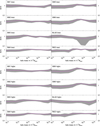 |
Fig. D.1 Mean biasing function b(m) for the mock galaxy samples SM1 to SM6 and the colour-selected samples BLUE and RED in the low-z (top) and high-z (bottom) redshift bin. The shaded regions indicate the 68% PI about the median for our fiducial mock survey. |
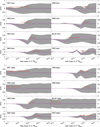 |
Fig. D.2 Excess variance V (m) for the mock galaxy samples SM1 to SM6 and the colour-selected samples BLUE and RED in the low-z (top) and high-z (bottom) redshift bin. The shaded regions indicate the 68% PI about the median for our fiducial mock survey. For each panel, the open square shows the median mass scale of the pivotal mass mpiv and its error bars the 68% PI. |
Summary of estimated model parameters in our simulated lensing analysis for the various galaxy samples and redshift bins.
References
- Abbott, T., Abdalla, F. B., Allam, S., et al. 2016, Phys. Rev. D, 94, 022001 [NASA ADS] [CrossRef] [Google Scholar]
- Aihara, H., Arimoto, N., Armstrong, R., et al. 2018, PASJ, 70, 54 [Google Scholar]
- Baldauf, T., Smith, R. E., Seljak, U., & Mandelbaum, R. 2010, Phys. Rev. D, 81, 063531 [NASA ADS] [CrossRef] [Google Scholar]
- Baldauf, T., Seljak, U., Smith, R. E., Hamaus, N., & Desjacques, V. 2013, Phys. Rev. D, 88, 083507 [NASA ADS] [CrossRef] [Google Scholar]
- Bardeen, J. M., Bond, J. R., Kaiser, N., & Szalay, A. S. 1986, ApJ, 304, 15 [NASA ADS] [CrossRef] [Google Scholar]
- Bartelmann, M., & Schneider, P. 2001, Phys. Rep., 340, 291 [NASA ADS] [CrossRef] [Google Scholar]
- Becker, M. R., Troxel, M. A., MacCrann, N., et al. 2016, Phys. Rev. D, 94, 022002 [NASA ADS] [CrossRef] [Google Scholar]
- Benson, A. J., Cole, S., Frenk, C. S., Baugh, C. M., & Lacey, C. G. 2000, MNRAS, 311, 793 [NASA ADS] [CrossRef] [Google Scholar]
- Bernstein, G. M., & Cai, Y.-C. 2011, MNRAS, 416, 3009 [NASA ADS] [CrossRef] [Google Scholar]
- Bertone, G., Hooper, D., & Silk, J. 2005, Phys. Rep., 405, 279 [NASA ADS] [CrossRef] [Google Scholar]
- Bridle, S., & King, L. 2007, New J. Phys., 9, 444 [NASA ADS] [CrossRef] [Google Scholar]
- Buddendiek, A., Schneider, P., Hildebrandt, H., et al. 2016, MNRAS, 456, 3886 [NASA ADS] [CrossRef] [Google Scholar]
- Bullock, J. S., Kolatt, T. S., Sigad, Y., et al. 2001, MNRAS, 321, 559 [Google Scholar]
- Cacciato, M., Lahav, O., van den Bosch, F. C., Hoekstra, H., & Dekel, A. 2012, MNRAS, 426, 566 [NASA ADS] [CrossRef] [Google Scholar]
- Chang, C., Pujol, A., Gaztañaga, E., et al. 2016, MNRAS, 459, 3203 [NASA ADS] [CrossRef] [Google Scholar]
- Clowe, D., Gonzalez, A., & Markevitch, M. 2004, ApJ, 604, 596 [NASA ADS] [CrossRef] [Google Scholar]
- Cole, S., Percival, W. J., Peacock, J. A., et al. 2005, MNRAS, 362, 505 [NASA ADS] [CrossRef] [Google Scholar]
- Comparat, J., Jullo, E., Kneib, J.-P., et al. 2013, MNRAS, 433, 1146 [NASA ADS] [CrossRef] [Google Scholar]
- Conselice, C. J., Wilkinson, A., Duncan, K., & Mortlock, A. 2016, ApJ, 830, 83 [Google Scholar]
- Cooray, A., & Sheth, R. 2002, Phys. Rep., 372, 1 [NASA ADS] [CrossRef] [Google Scholar]
- Dekel, A., & Lahav, O. 1999, ApJ, 520, 24 [NASA ADS] [CrossRef] [MathSciNet] [Google Scholar]
- Desjacques, V., Jeong, D., & Schmidt, F. 2016, Phys. Rep., submitted, [arXiv:1611.9787] [Google Scholar]
- Dodelson, S. 2003, Modern cosmology (Amsterdam: Academic Press) [Google Scholar]
- Einstein, A. 1917, in Sitzungsberichte der Königlich Preußischen Akademie der Wissenschaften (Berlin), 142 [Google Scholar]
- Eisenstein, D. J., & Hu, W. 1998, ApJ, 496, 605 [NASA ADS] [CrossRef] [Google Scholar]
- Erben, T., Hildebrandt, H., Miller, L., et al. 2013, MNRAS, 433, 2545 [NASA ADS] [CrossRef] [Google Scholar]
- Foreman, S., Becker, M. R., & Wechsler, R. H. 2016, MNRAS, 463, 3326 [NASA ADS] [CrossRef] [Google Scholar]
- Friedrich, O., Seitz, S., Eifler, T. F., & Gruen, D. 2016, MNRAS, 456, 2662 [NASA ADS] [CrossRef] [Google Scholar]
- Gao, L., & White, S. D. M. 2007, MNRAS, 377, L5 [NASA ADS] [CrossRef] [Google Scholar]
- Gelman, A., Carlin, J., Stern, H., & Rubin, D. 2003, Bayesian Data Analysis, 2nd Ed., Chapman & Hall/CRC Texts in Statistical Science (Taylor & Francis) [Google Scholar]
- Guzik, J., & Seljak, U. 2001, MNRAS, 321, 439 [NASA ADS] [CrossRef] [Google Scholar]
- Harnois-Déraps, J., van Waerbeke, L., Viola, M., & Heymans, C. 2015, MNRAS, 450, 1212 [NASA ADS] [CrossRef] [Google Scholar]
- Hartlap, J. 2009, Ph.D thesis, Universität Bonn, Germany, http://hss.ulb.uni-bonn.de/2009/1796/1796.htm [Google Scholar]
- Hartlap, J., Simon, P., & Schneider, P. 2007, A&A, 464, 399 [NASA ADS] [CrossRef] [EDP Sciences] [Google Scholar]
- Hartlap, J., Schrabback, T., Simon, P., & Schneider, P. 2009, A&A, 504, 689 [NASA ADS] [CrossRef] [EDP Sciences] [Google Scholar]
- Henriques, B. M. B., White, S. D. M., Thomas, P. A., et al. 2015, MNRAS, 451, 2663 [NASA ADS] [CrossRef] [Google Scholar]
- Hetterscheidt, M., Simon, P., Schirmer, M., et al. 2007, A&A, 468, 859 [NASA ADS] [CrossRef] [EDP Sciences] [Google Scholar]
- Heymans, C., Van Waerbeke, L., Miller, L., et al. 2012, MNRAS, 427, 146 [NASA ADS] [CrossRef] [Google Scholar]
- Heymans, C., Grocutt, E., Heavens, A., et al. 2013, MNRAS, 432, 2433 [NASA ADS] [CrossRef] [Google Scholar]
- Hilbert, S., Hartlap, J., White, S. D. M., & Schneider, P. 2009, A&A, 499, 31 [NASA ADS] [CrossRef] [EDP Sciences] [Google Scholar]
- Hildebrandt, H., Erben, T., Kuijken, K., et al. 2012, MNRAS, 421, 2355 [NASA ADS] [CrossRef] [Google Scholar]
- Hildebrandt, H., van Waerbeke, L., Scott, D., et al. 2013, MNRAS, 429, 3230 [NASA ADS] [CrossRef] [Google Scholar]
- Hildebrandt, H., Viola, M., Heymans, C., et al. 2017, MNRAS, 465, 1454 [Google Scholar]
- Hinshaw, G., Larson, D., Komatsu, E., et al. 2013, ApJS, 208, 19 [NASA ADS] [CrossRef] [Google Scholar]
- Hirata, C. M., & Seljak, U. 2004, Phys. Rev. D, 70, 063526 [NASA ADS] [CrossRef] [Google Scholar]
- Hockney, R. W., & Eastwood, J. W. 1981, Computer Simulation Using Particles Computer Simulation Using Particles, (New York: McGraw-Hill) [Google Scholar]
- Hoekstra, H., Yee, H. K. C., & Gladders, M. D. 2001, ApJ, 558, L11 [NASA ADS] [CrossRef] [Google Scholar]
- Hoekstra, H., van Waerbeke, L., Gladders, M. D., Mellier, Y., & Yee, H. K. C. 2002, ApJ, 577, 604 [NASA ADS] [CrossRef] [Google Scholar]
- Jing, Y. P. 2005, ApJ, 620, 559 [NASA ADS] [CrossRef] [Google Scholar]
- Joachimi, B., Mandelbaum, R., Abdalla, F. B., & Bridle, S. L. 2011, A&A, 527, A26 [NASA ADS] [CrossRef] [EDP Sciences] [Google Scholar]
- Joudaki, S., Blake, C., Johnson, A., et al., 2018, MNRAS, 474, 4894 [NASA ADS] [CrossRef] [Google Scholar]
- Jullo, E., Rhodes, J., Kiessling, A., et al. 2012, ApJ, 750, 37 [NASA ADS] [CrossRef] [Google Scholar]
- Kaiser, N. 1984, ApJ, 284, L9 [NASA ADS] [CrossRef] [Google Scholar]
- Kauffmann, G., Li, C., Zhang, W., & Weinmann, S. 2013, MNRAS, 430, 1447 [NASA ADS] [CrossRef] [Google Scholar]
- Kilbinger, M. 2015, Rep. Prog. Phys., 78, 086901 [Google Scholar]
- Kilbinger, M., Schneider, P., & Eifler, T. 2006, A&A, 457, 15 [NASA ADS] [CrossRef] [EDP Sciences] [Google Scholar]
- Kilbinger, M., Benabed, K., Guy, J., et al. 2009, A&A, 497, 677 [NASA ADS] [CrossRef] [EDP Sciences] [Google Scholar]
- Kilbinger, M., Wraith, D., Robert, C. P., et al. 2010, MNRAS, 405, 2381 [NASA ADS] [Google Scholar]
- Kilbinger, M., Fu, L., Heymans, C., et al. 2013, MNRAS, 430, 2200 [NASA ADS] [CrossRef] [Google Scholar]
- Kilbinger, M., Heymans, C., Asgari, M., et al. 2017, MNRAS, 472, 2126 [NASA ADS] [CrossRef] [Google Scholar]
- Kirk, D., Brown, M. L., Hoekstra, H., et al. 2015, Space Sci. Rev., 193, 139 [NASA ADS] [CrossRef] [Google Scholar]
- Kitching, T. D., Balan, S. T., Bridle, S., et al. 2012, MNRAS, 423, 3163 [NASA ADS] [CrossRef] [Google Scholar]
- Knight, K. 1999, Mathematical Statistics, Chapman & Hall/CRC Texts in Statistical Science (CRC Press) [CrossRef] [Google Scholar]
- Kuijken, K., Heymans, C., Hildebrandt, H., et al. 2015, MNRAS, 454, 3500 [NASA ADS] [CrossRef] [Google Scholar]
- Landy, S. D., & Szalay, A. S. 1993, ApJ, 412, 64 [NASA ADS] [CrossRef] [Google Scholar]
- Loverde, M., & Afshordi, N. 2008, Phys. Rev. D, 78, 123506 [NASA ADS] [CrossRef] [Google Scholar]
- Mandelbaum, R., Hirata, C. M., Ishak, M., Seljak, U., & Brinkmann, J. 2006, MNRAS, 367, 611 [NASA ADS] [CrossRef] [Google Scholar]
- Martino, L., & Read, J. 2013, Comput. Stat., 28, 2797 [CrossRef] [Google Scholar]
- Mehta, K. T., Seo, H.-J., Eckel, J., et al. 2011, ApJ, 734, 94 [NASA ADS] [CrossRef] [Google Scholar]
- Mo, H., van den Bosch, F. C., & White, S. 2010, Galaxy Formation and Evolution [CrossRef] [Google Scholar]
- Munshi, D., Valageas, P., van Waerbeke, L., & Heavens, A. 2008, Phys. Rep., 462, 67 [NASA ADS] [CrossRef] [Google Scholar]
- Navarro, J. F., Frenk, C. S., & White, S. D. M. 1996, ApJ, 462, 563 [NASA ADS] [CrossRef] [Google Scholar]
- Peacock, J. A., & Smith, R. E. 2000, MNRAS, 318, 1144 [NASA ADS] [CrossRef] [Google Scholar]
- Peebles, P. J. E. 1980, The large-scale structure of the Universe (Princeton University Press) [Google Scholar]
- Pen, U.-L., Lu, T., van Waerbeke, L., & Mellier, Y. 2003, MNRAS, 346, 994 [NASA ADS] [CrossRef] [Google Scholar]
- Planck Collaboration XIII. 2016, A&A, 594, A13 [NASA ADS] [CrossRef] [EDP Sciences] [Google Scholar]
- Prat, J., Sánchez, C., Miquel, R., et al. 2018, MNRAS, 473, 1667 [NASA ADS] [CrossRef] [Google Scholar]
- Pujol, A., Chang, C., Gaztañaga, E., et al. 2016, MNRAS, 462, 35 [NASA ADS] [CrossRef] [Google Scholar]
- Reyes, R., Mandelbaum, R., Seljak, U., et al. 2010, Nature, 464, 256 [NASA ADS] [CrossRef] [PubMed] [Google Scholar]
- Saghiha, H., Simon, P., Schneider, P., & Hilbert, S. 2017, A&A, 601, A98 [NASA ADS] [CrossRef] [EDP Sciences] [Google Scholar]
- Schneider, P. 1998, ApJ, 498, 43 [NASA ADS] [CrossRef] [Google Scholar]
- Schneider, P., Kochanek, C., & Wambsganss, J. 2006, Gravitational lensing: strong, weak and micro, Saas-Fee Advanced Course: Swiss Society for Astrophysics and Astronomy (Springer) [Google Scholar]
- Schneider, P., van Waerbeke, L., Kilbinger, M., & Mellier, Y. 2002, A&A, 396, 1 [NASA ADS] [CrossRef] [EDP Sciences] [Google Scholar]
- Seljak, U. 2000, MNRAS, 318, 203 [NASA ADS] [CrossRef] [Google Scholar]
- Sellentin, E., & Heavens, A. F. 2016, MNRAS, 456, L132 [NASA ADS] [CrossRef] [Google Scholar]
- Semboloni, E., Hoekstra, H., Schaye, J., van Daalen, M. P., & McCarthy, I. G. 2011, MNRAS, 417, 2020 [NASA ADS] [CrossRef] [Google Scholar]
- Sheth, R. K., & Tormen, G. 1999, MNRAS, 308, 119 [NASA ADS] [CrossRef] [Google Scholar]
- Simon, P. 2012, A&A, 543, A2 [NASA ADS] [CrossRef] [EDP Sciences] [Google Scholar]
- Simon, P. 2013, A&A, 560, A33 [NASA ADS] [CrossRef] [EDP Sciences] [Google Scholar]
- Simon, P., Hetterscheidt, M., Schirmer, M., et al. 2007, A&A, 461, 861 [NASA ADS] [CrossRef] [EDP Sciences] [Google Scholar]
- Simon, P., Hetterscheidt, M., Wolf, C., et al. 2009, MNRAS, 398, 807 [NASA ADS] [CrossRef] [Google Scholar]
- Simon, P., Erben, T., Schneider, P., et al. 2013, MNRAS, 430, 2476 [NASA ADS] [CrossRef] [EDP Sciences] [Google Scholar]
- Simon, P., Semboloni, E., van Waerbeke, L., et al. 2015, MNRAS, 449, 1505 [NASA ADS] [CrossRef] [Google Scholar]
- Simon, P., Saghiha, H., Hilbert, S., Schneider, P., & Boever, C. 2017, A&A, submitted [arXiv:1710.099027] [Google Scholar]
- Singh, S., Mandelbaum, R., Seljak, U., Slosar, A., & Vazquez Gonzalez, J. 2017, MNRAS, 471, 3827 [NASA ADS] [CrossRef] [Google Scholar]
- Smith, R. E., Peacock, J. A., Jenkins, A., et al. 2003, MNRAS, 341, 1311 [NASA ADS] [CrossRef] [Google Scholar]
- Somerville, R. S., Lemson, G., Sigad, Y., et al. 2001, MNRAS, 320, 289 [NASA ADS] [CrossRef] [Google Scholar]
- Springel, V., White, S. D. M., Jenkins, A., et al. 2005, Nature, 435, 629 [NASA ADS] [CrossRef] [PubMed] [Google Scholar]
- Springel, V., Frenk, C. S., & White, S. D. M. 2006, Nature, 440, 1137 [NASA ADS] [CrossRef] [PubMed] [Google Scholar]
- Springel, V., Pakmor, R., Pillepich, A., et al. 2018, MNRAS, 475, 676 [NASA ADS] [CrossRef] [Google Scholar]
- Takahashi, R., Sato, M., Nishimichi, T., Taruya, A., & Oguri, M. 2012, ApJ, 761, 152 [NASA ADS] [CrossRef] [Google Scholar]
- Tegmark, M., & Bromley, B. C. 1999, ApJ, 518, L69 [NASA ADS] [CrossRef] [Google Scholar]
- Tegmark, M., & Peebles, P. J. E. 1998, ApJ, 500, L79 [NASA ADS] [CrossRef] [Google Scholar]
- Tinker, J. L., Weinberg, D. H., Zheng, Z., & Zehavi, I. 2005, ApJ, 631, 41 [NASA ADS] [CrossRef] [Google Scholar]
- Troxel, M. A.,& Ishak, M. 2015, Phys. Rep., 558, 1 [NASA ADS] [CrossRef] [Google Scholar]
- van Uitert, refgnE., Joachimi, B., Joudaki, S., et al. 2018, MNRAS, 476, 4662 [NASA ADS] [CrossRef] [Google Scholar]
- van Waerbeke,L. 1998, A&A, 334, 1 [NASA ADS] [Google Scholar]
- Velander, M., van Uitert, E., Hoekstra, H., et al. 2014, MNRAS, 437, 2111 [NASA ADS] [CrossRef] [Google Scholar]
- Weinberg, D. H., Davé, R., Katz, N., & Hernquist, L. 2004, ApJ, 601, 1 [NASA ADS] [CrossRef] [Google Scholar]
- Ziour, R., & Hui, L. 2008, Phys. Rev. D, 78, 123517 [Google Scholar]
All Tables
Selection criteria applied to our mock galaxies to emulate stellar-mass samples consistent with SES13 and for the two additional colour-selected samples RED and BLUE.
Overview of the reconstruction accuracy by listing the mean fractional errors σb,r and extreme outliers Δb,r of the inferred biasing functions b(k) and r(k), respectively, in %.
Summary of possible systematic errors and their expected impact on the reconstruction of b(k) or r(k) for a WMAP9 cosmology and our galaxy samples.
Results of KS-test for Gaussianity for three kinds of the aperture statistic at scales θ = 2, 20, 60, 120 arcmin (in this order).
Summary of estimated model parameters in our simulated lensing analysis for the various galaxy samples and redshift bins.
All Figures
|
Fig. 1 Models of the probability densities pd(z) of galaxy redshifts in our lens samples SM1 to SM6, RED and BLUE (two top panels), and the density ps (z) of the source sample (bottom panel). |
| In the text | |
|
Fig. 2 Levels of GI and II contributions to |
| In the text | |
|
Fig. 3 Relative change of |
| In the text | |
|
Fig. 4 Relative errors in the aperture statistics due to magnification bias of the lenses. Left: errors for |
| In the text | |
|
Fig. 5 Weight Wm(k) of the two-halo term in the matter-power spectrum for varying redshifts z. |
| In the text | |
|
Fig. 6 Family of templates b(k) (black lines) and r(k) (red lines) for the range of wave numbers k in the top axis; the left-hand y axis applies to the panels in the first column, the right-hand axis to the second column. The aperture scale θap = 4.25∕(k fK(zd)) (bottom axis) crudely traces the projected b2D(θap) and r2D(θap) for lens galaxies at zd = 0.3. Each panel varies only one template parameter. See text for more details. |
| In the text | |
|
Fig. 7 Biasing functions b(k) (left panels) and r(k) (right panels) for all mock galaxy samples SM1 to SM6 and two redshift bins. The top figure is for the low-z samples ( |
| In the text | |
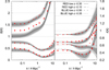 |
Fig. 8 As in Fig. 7 but now for the colour-selected samples RED and BLUE. |
| In the text | |
|
Fig. 9 Average error in the galaxy-bias normalisation fb (x-axis) and fr (y-axis). The points show as indistinguishable the errors of all galaxy samples SM1-4, BLUE, and RED together; the point styles indicate the redshift bin and what is varied. Symbols as in the figure key indicate the low-z samples, inverted symbols indicate the high-z samples (e.g. solid and open circles). The “cosmo” and “sampling p(z)” data points reuse the same galaxy samples many times with random normalisation errors. The solid line marks the estimated error for high-z samples dueto the baryon uncertainty. The fiducial cosmology is WMAP9. See text for more details. |
| In the text | |
|
Fig. 10 Systematic relative errors in b2D(θap) (low-z and high-z) and r2D(θap) (only low-z) when II andGI terms are ignored in the normalisation of the galaxy bias. Different lines show predictions for different values of Aia with sourcesas in our mock survey. The fiducial cosmology is WMAP9. |
| In the text | |
|
Fig. 11 As in Fig. 10 but now for r2D(θap) high-z. Shown are results from SM4 but the values are similar for the other samples. |
| In the text | |
|
Fig. 12 Correlation matrix Cij of measurement errors for three kinds of aperture statistics of FORE-I lenses in the GaBoDS analysis. The integers on the two axes inside the matrix refer to either the i or j index. Values 1 ≤ k ≤ 6 for k being either i or j refer to errors of |
| In the text | |
|
Fig. 13 Left:posterior model of r2D(θap) (top) and b2D(θap) (bottom) based on the GaBoDS measurements FORE-I (shaded regions with 68% and 95% PI). Shown as black open squares are the median values and a 68% interval around the median for the measured b2D and r2D; the open circles indicate the mean. The red-star data points H+02 show the measurements by Hoekstra et al. (2002) for comparison. Right: 68% PI posterior of the excess HOD variance V (m) with open box for the mass scale of the pivotal mass mpiv (top); 68% PI posterior of the mean biasing function b(m) and fcen as open triangle (bottom). The fiducial model has WMAP9 parameters. |
| In the text | |
|
Fig. 14 Reconstructed biasing functions of FORE-I galaxies in GaBoDS. Shown are the 68% and 95% PI of b(k) in the bottom panel and that of r(k) in the top panel. The biasing function are an average over the redshift range 0.34 ±0.16 for a WMAP9 cosmology. The red data points show the biasing function of BLUE low-z, which have asimilar b(m). |
| In the text | |
|
Fig. D.1 Mean biasing function b(m) for the mock galaxy samples SM1 to SM6 and the colour-selected samples BLUE and RED in the low-z (top) and high-z (bottom) redshift bin. The shaded regions indicate the 68% PI about the median for our fiducial mock survey. |
| In the text | |
|
Fig. D.2 Excess variance V (m) for the mock galaxy samples SM1 to SM6 and the colour-selected samples BLUE and RED in the low-z (top) and high-z (bottom) redshift bin. The shaded regions indicate the 68% PI about the median for our fiducial mock survey. For each panel, the open square shows the median mass scale of the pivotal mass mpiv and its error bars the 68% PI. |
| In the text | |
Current usage metrics show cumulative count of Article Views (full-text article views including HTML views, PDF and ePub downloads, according to the available data) and Abstracts Views on Vision4Press platform.
Data correspond to usage on the plateform after 2015. The current usage metrics is available 48-96 hours after online publication and is updated daily on week days.
Initial download of the metrics may take a while.