| Issue |
A&A
Volume 612, April 2018
|
|
|---|---|---|
| Article Number | A103 | |
| Number of page(s) | 11 | |
| Section | Interstellar and circumstellar matter | |
| DOI | https://doi.org/10.1051/0004-6361/201732238 | |
| Published online | 08 May 2018 | |
Radio outburst from a massive (proto)star
When accretion turns into ejection★
1
INAF, Osservatorio Astrofisico di Arcetri,
Largo E. Fermi 5,
50125
Firenze, Italy
e-mail: This email address is being protected from spambots. You need JavaScript enabled to view it.
2
Institut de Radioastronomie Millimétrique (IRAM),
300 rue de la Piscine,
38406
Saint-Martin d’Hères, France
3
Max Planck Institut für Radioastronomie,
Auf dem Hügel 69,
53121
Bonn, Germany
4
Dublin Institute for Advanced Studies, Astronomy & Astrophysics Section,
31 Fitzwilliam Place,
Dublin
2, Ireland
5
Thüringer Landessternwarte Tautenburg,
Sternwarte 5,
07778
Tautenburg, Germany
Received:
6
November
2017
Accepted:
21
December
2017
Abstract
Context. Recent observations of the massive young stellar object S255 NIRS 3 have revealed a large increase in both methanol maser flux density and IR emission, which have been interpreted as the result of an accretion outburst, possibly due to instabilities in a circumstellar disk. This indicates that this type of accretion event could be common in young/forming early-type stars and in their lower mass siblings, and supports the idea that accretion onto the star may occur in a non-continuous way.
Aims. As accretion and ejection are believed to be tightly associated phenomena, we wanted to confirm the accretion interpretation of the outburst in S255 NIRS 3 by detecting the corresponding burst of the associated thermal jet.
Methods. We monitored the radio continuum emission from S255 NIRS 3 at four bands using the Karl G. Jansky Very Large Array. The millimetre continuum emission was also observed with both the Northern Extended Millimeter Array of IRAM and the Atacama Large Millimeter/Submillimeter Array.
Results. We have detected an exponential increase in the radio flux density from 6 to 45 GHz starting right after July 10, 2016, namely ~13 months after the estimated onset of the IR outburst. This is the first ever detection of a radio burst associated with an IR accretion outburst from a young stellar object. The flux density at all observed centimetre bands can be reproduced with a simple expanding jet model. At millimetre wavelengths we infer a marginal flux increase with respect to the literature values and we show this is due to free–free emission from the radio jet.
Conclusions. Our model fits indicate a significant increase in the jet opening angle and ionized mass loss rate with time. For the first time, we can estimate the ionization fraction in the jet and conclude that this must be low (<14%), lending strong support to the idea that the neutral component is dominant in thermal jets. Our findings strongly suggest that recurrent accretion + ejection episodes may be the main route to the formation of massive stars.
Key words: stars: early-type / stars: formation / stars: winds, outflows / ISM: jets and outflows
Based on observations carried out with the VLA, IRAM/NOEMA, and ALMA.
This article is dedicated to the memory of MalcolmWalmsley, who passed away before the present study could be completed. Without his insights and enlightened advice this work would have been impossible. We will always remember all the stimulating discussions with him, as well as his delightful personality.
© ESO 2018
1 Introduction
The accretion phenomenon has recently gained importance not only in the formation process of solar-type stars, but also across the whole stellar mass spectrum. Growing evidence of the presence of disks around B-type and even O-type stars lends strong support to the hypothesis that even the most massive stars may form through disk-mediated accretion, as the latter can overcome their powerful radiation pressure (Krumholz et al. 2007; Kuiper et al. 2010; Peters et al. 2010). While most theoretical models assume a smooth, steady accretion flow onto the star, it is very likely that in real life the flow is much more irregular, due to disk inhomogeneities and fragmentation. This scenario is suggested by the detection of sudden increases in the stellar luminosity in low-mass (proto)stars, which hint at episodic accretion events. These phenomena are known as FUor and EXor outbursts and consist of an increase of up to 6 mag in the young stellar object (YSO) luminosity in the optical and near-IR, which corresponds to an increase in the mass accretion rate of up to ~ 10−4 M⊙ yr−1 (Audard et al. 2014). Correspondingly, these accretion events are believed to trigger an increase in the mass ejection rate.
While recent studies have corroborated the idea that accretion bursts take place through a broad range of stellar masses (Acosta-Pulido et al. 2007; Caratti o Garatti et al. 2011; Contreras Peña et al. 2017), it is not obvious that they should also occur in early-type stars, namely for stellar masses in excess of ~6 M⊙. However, evidence of such a burst was reported by Tapia et al. (2015) in V723 Car, a YSO with a relatively high luminosity (~ 4 × 10³ L⊙).
More recently, Fujisawa et al. (2015) detected a powerful methanol maser flare at 6 GHz towards the 20 M⊙ YSO S255 NIRS 3, located at a distance of 1.78 kpc (Burns et al. 2016). Since CH3OH class II masers are believed to be radiatively pumped, follow-up observations at IR wavelengths were performed, which indeed revealed a dramatic brightening of the source of 2.9 mag and 3.5 mag at K and H bands, respectively (Stecklum et al. 2016), and a corresponding increase in bolometric luminosity of ~ 1.3 × 10⁵ L⊙ (Caratti o Garatti et al. 2017). Our study has shown that such an increase is likely driven by an accretion burst of ~ 5 × 10⁻³ M⊙ yr−1 that occurred around mid-June 2015. This result is consistent with the proposed existence of a disk-jet system in S255 NIRS 3 (Wang et al. 2011; Boley et al. 2013; Zinchenko et al. 2015), which may be mediating the accretion process.
Finally, our high angular resolution observations (from 1 mas to 1′′) of the methanol maser flare revealed a substantial change in the circumstellar environment of the bursting source. In particular, the main pre-burst maser cluster, located close to the radio continuum peak, is no longer detected during the burst. Instead, a new extended plateau has formed at a projected separation of 500–1000 au from the YSO (Moscadelli et al. 2017).
Since November 2015 we have been performing multi-epoch observations of the source in a variety of tracers from the IR to the radio, with a number of instruments such as the VLT, IRTF, 2.2 m Calar Alto, Effelsberg, SOFIA, and the GMRT. In particular, we are monitoring the centimetre and millimetre continuum emission by means of the Karl G. Jansky Very Large Array (VLA), the Northern Extended Millimeter Array (NOEMA) of IRAM, and the Atacama Large Millimeter/Submillimeter Array (ALMA). Our main goal was to establish whether the accretion burst had boosted the radio thermal jet visible in archival VLA images of S255 NIRS 3 (see Fig. 1a). Since accretion and ejection are believed to be closely related phenomena during the star formation phase, our expectation was to detect a sudden brightening of the radio emission from the jet itself as a consequence of the accretion burst revealed from the IR brightening. Indeed, our monitoring resulted in the first ever detection of a radio burst associated with an IR outburst, and we report on our finding in the present article.
In Sect. 2 we give the observational details, while the results obtained are described in Sect. 3 and analyzed through a suitable model in Sect. 4. Finally, the conclusions are drawn in Sect. 5.
2 Observations and data analysis
In the following, we report on the VLA data obtained in 2016 and the ALMA and IRAM/NOEMA data acquired between December 2016 and February 2017.
In all cases, the phase centre of the observations was set at the coordinates α(J2000) = 06h12m54. s02, δ(J2000) = 17°59′23.′′1.
2.1 Very Large Array
S255 NIRS 3 was observed using the VLA of the National Radio Astronomy Observatory (NRAO) at five epochs during 2016 (project code: 16A-424): in C configuration on March 11, in B configuration on July 10 and August 1, and in A configuration on October 15, November 24, and December 27.
Each observing epoch lasted 1.73 h and recorded the signal at 6.0, 10.0, 22.2, and 45.5 GHz. We employed the capabilities of the WIDAR correlator, which permits recording dual polarization across a total bandwidth per polarization of 2 GHz, by using two IFs, each comprising eight adjacent 128 MHz sub-bands. The total observing bandwidth (per polarization) was 4.1 GHz (with 2 IFs) at 6.0 and 10.0 GHz, and 8.0 GHz (with 4 IFs) at 22 and 45 GHz. The primary flux calibrator was 3C48, and the phase-calibrator was J0559 + 2353, separated by ~ 7° from the target.
Calibration and imaging were performed with the CASA2 software, by using different versions (from 4.3.1 to 4.5.2) of the JVLA data reduction pipeline. We estimate a calibration accuracy of ~10%. The continuum images were constructed using natural or Briggs robust = 0 weighting. Table 1 reports the mean synthesized beam widths at half power, at the five observing epochs. The rms noise level of the continuum images is close to the expected thermal noise, in the range 10–20 μJy beam−1 at 6, 10 GHz, and 22 GHz, while it is significantly higher, 50–100 μJy beam−1 at 45 GHz, where atmospheric phase noise is dominant. At 22 and 45 GHz, we self-calibrated the compact continuum emission, improving the dynamic range of the image by a factor of a few.
Flux densities measured towards the central core of S255 NIRS 3 with the VLA, IRAM/NOEMA, and ALMA at different epochs, and corresponding mean synthesized beams.
2.2 IRAM/NOEMA
We observed S255 NIRS 3 with the interferometer on January 23 and February 15, 2017. The array consisted of eight elements in the compact D configuration. The bandpass and phase calibrator were J0507 + 179, while flux calibration was performed by means of observationsof LkHa101. We used the wideband correlator (WideX) to obtain a measurement of the continuum emission at both 3.4 and 2 mm. For this purpose the receivers were tuned to cover a 3.6 GHz wide band centred at 87 and 150 GHz. All observationswere performed with on-source integration times of 10 min. Observations were carried out first at 3.4 mm, and were immediatelyfollowed by observations at 2 mm.
Data calibration and imaging were made through standard procedures, using the GILDAS package3. All maps were made with natural weighting, resulting in a synthesized beam with full widths at half power of 5.′′ 0 × 3.′′5 with PA = 195° at 3.4 mm and 3.′′ 0 × 1.′′9 with PA = 0° at 2 mm in January, and 5.′′ 1 × 3.′′3 with PA 193° at 3.4 mm and 2.′′ 9 × 1.′′8 with PA = 11° at 2 mm in February. The continuum maps were obtained by visually inspecting the data cubes and selecting channels with no evidence of line emission. These channels were then averaged in the u, v domain and pure continuum images were made from the averaged u, v data. The resulting continuum bandwidth was 682 MHz at 3.4 mm and 379 MHz at 2 mm. The thermal noise level is typically 0.1 mJy/beam at 3.4 mm and 0.3 mJy/beam at 2 mm. Flux calibration is accurate to within 20% at both wavelengths.
2.3 Atacama Large Millimeter/Submillimeter Array
S255 NIRS 3 was observed with ALMA at band 3 on December 16, 2016. The array consisted of 45 antennas arranged in a configuration with baselines from ~20 to ~400 m, which provides sensitivity to structures up to ~30′′. Since our main goal was to image the continuum emission, we configured the correlator to cover a total bandwidth of ~8 GHz with four units of 2 GHz, in double polarization, centred at 85.2, 87.2, 97.2, and 99.2 GHz. We chose the maximum possible spectral resolution of 0.49 MHz in order to identify strong lines that could significantly contaminate the continuum measurement. For flux and bandpass calibration we used the strong calibrators J0510 + 1800 and J0750 + 1231, while the phase calibrator J0613 + 1708 was separated by <1° from our target. Calibration and imaging were performed with the CASA software by employing the ALMA data reduction pipeline. We estimate a calibration error of ~20%.
A data cube was created from each 2 GHz correlator unit with natural weighting. In order to obtain a pure continuum image, we adopted the STATCONT method by Sánchez-Monge et al. (2018), which automatically identifies line-free channels in the cubes. In this way four continuum maps were obtained at the four centre frequencies of the correlator units. The synthesized half-power beam widths and the 1σ RMS noise ranged respectively from 2.′′ 21 × 2.′′12 to 2.′′ 61 × 2.′′45, and from 0.34 to 0.61 mJy/beam, depending on the frequency.
Finally, for each continuum image the flux density of S255 NIRS 3 was computed by integrating the emission over the corresponding core (indicated with SMA1 by Zinchenko et al. 2012). Since pairs of correlator units are close in frequency, we computed a mean value of the flux for each pair, thus obtaining a continuum flux density of ~73 mJy at 86.2 GHz and ~90 mJy at 98.2 GHz.
3 Results
3.1 Centimetre emission
Our VLA monitoring started on March 11, 2016, about 9 months after the estimated onset of the outburst (mid-June 2015; see Caratti o Garatti et al. 2017). As illustrated in Fig. 1, comparison with VLA archival data obtained at the same frequency on August 27, 1990 (project AM301), with similar angular resolution reveals some structural change. In the middle panel of thefigure we also show the archival map after smoothing to the same angular resolution as our new data.
All images clearly outline an elongated structure consisting of a central bright core, coincident with the NIRS 3 infrared source, plus two symmetrically displaced knots to the NE and SW. We interpret this structure as a bipolar radio jet, identified by us for the first time. Indeed, the jet lobes are oriented in the same direction as the axis of the bipolar outflow identified by Zinchenko et al. (2015). Moreover, the two knots coincide with FeII 1.64 μm emission detected by Wang et al. (2011), which lends further support to our interpretation.
The archival images in Figs. 1a and 1b differ from that in Fig. 1c in the SW lobe, which appears split into two knots. Moreover, the central core looks fainter in our new image (taken on March 11, 2016) with a total flux density ~1.7 times less than that measured in 1990. A decrease of the same amount is observed in the NE knot, whereas the total flux from all the SW knots (~0.9 mJy) has remained basically the same.
We conclude that in 26 yr the radio jet has undergone significant morphological changes over an angular scale comparable to the size of the SW lobe, i.e. ~2′′ or ~3600 au on the plane of the sky. This implies that the ionized gas in the jet is moving at an average speed on the plane of the sky of at least ~660 km s−1. However, the observed changes do not support the occurrence of a radio burst at the current epoch because the radio emission from the whole jet and, in particular, from the central core has not increased. Unlike the SW lobe, the shape of the NE lobe has remained basically the same, as has its distance from the central source. This suggests that any ejection episode might be highly asymmetric,as also discussed by other authors (e.g. Melnikov et al. 2008, 2009; Caratti o Garatti et al. 2013; Cesaroni et al. 2013).
The second epoch of our VLA monitoring (July 10, 2016) has confirmed the lack of brightening of the emission. The flux density from the central core (and that of the other two knots) is unchanged, within the uncertainties, with respect to that measured atthe same frequency in March. This can be seen in Table 1 where the fluxes measured from NIRS 3 during our monitoring are given. The only significant change is seen at 46 GHz, where the flux density is less intense in July than in March. However, this decrease is likely due to the more extended configuration (B-array) of the second-epoch observations, which resolves out the dust emission from the hot molecular core enshrouding NIRS 3.
At the third epoch (August 1, 2016) we suddenly detected an increase in the radio emission from the central core of NIRS 3 at all observed frequencies. We note that at the same epoch no changes were detected from the NE and SW knots. This brightening is undoubtedly real and not due to a calibration error because we observe an increase of a factor ~1.6 in the ratio between the flux of the central core and that of the two radio knots. This can be easily seen by visual comparison between theVLA maps made in July and those made in August (see Fig. 2). We stress that the same array configuration (B) was used at both epochs, hence the difference in flux cannot be attributed to different uv-coverage.
Since no variation is detected from the NE and SW knots, hereafter we will focus only on the central radio core, NIRS 3, and we refer to it simply as “the jet”.
It is interesting to note that the jet flux measured in August at 10 GHz (1.8 mJy; see Table 1) is equal to the value obtained from the archival data in 1990 (Fig. 1a). This might indicate that the source underwent other outburst episodes in the past, consistent with a scenario where accretion occurs mainly in an irregular way. A similar conclusion was attained by Burns et al. (2016), who identify the signposts of three distinct ejection events from S255 NIRS 3.
Figure 3 illustrates the evolution of the flux density of NIRS 3 from March to December 2016. As already noted, after an initial quiescent phase, the flux rose between July and August, undergoing an exponential increase. The dashed lines in the figure are fits to the expressions of the flux density, Sν, as a function of time, t,
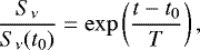 (1)
(1)
where we assume t0 = 0 on July 10 and the timescale T is the free parameter of the fit. The value of T ranges from 58 days (for the 45 GHz data) to 82 days (for the 22 GHz data), with a mean value of 77 days.
Clearly, the fits in Fig. 3 indicate that the radio burst has indeed started very close to t = 0, i.e. July 10, 2016. Therefore, we assume that the increase in the radio flux became detectable right after this date.
Assuming that the radio burst is due to expansion of the jet on a timescale equal to T, with a typical expansion speed of 660 km s−1 (see above), we find a corresponding spatial scale of ~30 au. While this value has no precise correspondence with a specific geometrical feature of the jet, nonetheless it indicates that the jet is very compact and arises close to the circumstellar disk.
We can also use the expansion speed to derive a rough estimate of the maximum jet size, at the most recent observing epoch (December 27, 2016). With a time lag of ~560 days from the estimated beginning of the outburst (mid-June 2015), the jet should have expanded up to ~210 au or 0.′′12 (assuming that accretion and ejection occur at the same time).
A jet of this size should be barely resolved on our maps at the highest frequencies. Indeed, at 22.2 GHz we do reveal an elongated structure just in the direction of the NE knot of the larger scale radio jet. Figure 4 shows the corresponding map, where the low-level emission has been suitably enhanced. The approximate size on the plane of the sky is ~300 au. We note that the same structure is not detected at 7 mm because at this band the uv-coverage and hence the corresponding image quality has been significantly degraded due to heavy flagging of the data. This finding provides us with direct evidence of the existence of an expanding jet on scales of a few 100 au.
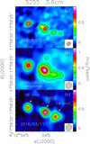 |
Fig. 1 Panel a: VLA archival image obtained on August 27, 1990, at 3.6 cm with the C-array configuration. The values of the contour levels are drawn in the corresponding colour scales to the right. The full width at half power of the synthesized beam is shown in the bottom right. Panel b: Same as the top panel, after smoothing to the resolution of our new 3 cm image. Panel c: Same as the other panels, but for our new 3 cm image obtained on March 11, 2016, with the C-array configuration. The bipolar structure of the jet is shown, consisting of a central core associated with NIRS 3 and two main knots to theNE and SW. |
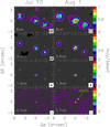 |
Fig. 2 Maps of the S255 NIRS 3 region at centimetre wavelengths obtained with the VLA on July 10 (left panels) and August 1 (right panels), 2016. The offsets are computed with respect to the phase centre of the observations, i.e. 06h 12m 54. s02, 17°59′23.′′1. The corresponding synthesized beams are shown at the bottom right of each panel. The values of the contour levels are marked in the colour scales to the right, and in all cases the lowest contour is >4σ. We note thebrightening of NIRS 3 at all frequencies. |
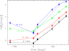 |
Fig. 3 Observed radio flux densities of NIRS 3 as a function of time, with t = 0 corresponding to the second epoch of our monitoring (July 10, 2016). The solid lines connect fluxes observed at the same frequency, which is given beside each curve. The dashed lines are the fits assuming exponential dependence on t according to Eq. (1). |
3.2 Millimetre emission
Our monitoring with the IRAM/NOEMA and ALMA interferometers provides flux density measurements starting from December 16, 2016. In addition to this observation, we report on two more epochs, namely January 23 and February 15, 2017. These data allow us to establish that the millimetre emission from source NIRS 3 is basically constant in time. Our angular resolution is sufficient to resolve the hot molecular core associated with NIRS 3, named SMA1 by Zinchenko et al. (2012), from the nearby fainter core, named SMA2 by the same authors. In Table 1 we give the mm flux densities of NIRS 3 at the different epochs. Clearly, no change is seen within a calibration error of ~20%.
As already done for the VLA data, it is worth comparing our flux density measurements with those from the literature. However, unlike the case of the centimetre emission, direct comparison with the literature values is impossible because they were taken at shorter wavelengths. Moreover, a variety of array configurations were used, which further complicates the comparison of literature fluxes from different authors.
In an attempt to overcome this problem, we have collected all the results from observations of S255 NIRS 3 performed with the same instrument, the Submillimeter Array (SMA). These are given in Table 2, with the observing frequency and angular resolution. The large spread of the flux densities at the same frequency is due to the more extended array configurations which provide better angular resolutions, but also resolve out part of the emission. To correct for this effect, we assume that the largest angular scale, Θ L, that can beimaged by the interferometer is proportional to the synthesized beam, Θ B. This assumption is reasonable for the given interferometer. We also assume that the flux density measured by the interferometer at a given frequency towards a given source scales as
 (2)
(2)
with α > 0. This empirical relation expresses the concept that the lower the resolution, the smaller the amount of flux resolved out by the interferometer.
To determine α we have used the fluxes from the literature measured at the same frequency with different resolutions. In Fig. 5a, we plot the flux density versus the half-power width of the synthesized beam for all measurements from Table 2 at 225 GHz. We have also included the 230 GHz flux density from Wang et al. (2011) after scaling it to 225 GHz, assuming a spectral index4 of 2. Fitting Eq. (2) to this plot, we obtain the expression
![Mathematical equation: \begin{equation*} S_{\textrm{225\,GHz}}(\textrm{mJy}) = 115.5 \, \left[\mathrm\Theta_{\textrm{B}}(\textrm{arcsec})\right]^{0.8}.\end{equation*}](/articles/aa/full_html/2018/04/aa32238-17/aa32238-17-eq4.png) (3)
(3)
This expression applies only to the range of fluxes and ΘB in Fig. 5a. Any extrapolation beyond these limits or application of Eq. (3) to interferometers other than the SMA is unreliable.
Using this equation, we can scale all fluxes in the table to the same angular resolution. We adopt the lowest resolution in Table 2, ΘB = 3.′′37 because thisis the closest to the resolution of our ALMA and IRAM/NOEMA images and likely recovers most of the flux from the NIRS 3 hot molecular core.
From the corrected fluxes we can then derive the spectral slope Sν ∝ νβ. This is done in Fig. 5b, where the empty points indicate the original fluxes measured with the SMA and the solid points those after scaling for  . The best fit to the corrected fluxes is
![Mathematical equation: \begin{equation*} S_{\nu}(\textrm{mJy}) = 3.89\times10^{-3} \, \left[\nu(\textrm{GHz})\right]^{2.08}.\end{equation*}](/articles/aa/full_html/2018/04/aa32238-17/aa32238-17-eq6.png) (4)
(4)
This expression allows extrapolation to the bands covered by our observations and comparison to the corresponding flux densities. The extrapolated fluxes at 2 mm and 3 mm are 20–40% less than those measured by us. Even allowing for a 20% calibration error, this difference suggests that the millimetre source could be now slightly brighter than in the pre-burst phase. We discuss this possibility in Sect. 4.2.
Flux densities measured at mm wavelengths towards S255 NIRS 3 with the SMA by various authors.
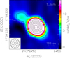 |
Fig. 4 Continuum map at 22.2 GHz of the radio source NIRS 3 obtained at the fifth epoch of our monitoring (December 27, 2016). The image has been saturated to emphasize the elongated structure. The dashed line denotes thedirection connecting NIRS 3 to the NE knot of the large-scale radio jet. Contour levels range from 0.6 (7σ) to 13.2 in steps of 1.8 mJy/beam. The ellipse in the bottom left denotes the synthesized beam. |
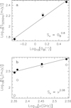 |
Fig. 5 Panel a: Flux densities at 225 GHz and 230 GHz from Table 2 versus the full width at half power of the corresponding synthesized beam. The 230 GHz flux (empty point) has been scaled to 225 GHz (solid point) assuming Sν ∝ ν2. The straight line is the linear fit (in the logarithmic plot) to the solid points, based on Eq. (3). Panel b: Flux densities from Table 2 as a function of frequency before (empty points) and after (solid points) scaling the fluxes to an angular resolution of 3.′′ 37 (see text) with Eq. (3). The straight line is the linear fit (in the logarithmic plot) to the solid points, based on Eq. (4). |
4 Interpretation: an expanding jet model
We wish to demonstrate that an expanding thermal jet boosted by the accretion outburst is a viable explanation for the observed exponential increase in the radio emission from S255 NIRS 3.
From the archival data we know that the radio jet was already present at the moment of the radio burst, which means that any realistic jet model should consider a scenario where a pre-existent thermal jet is suddenly perturbed by a massive ejection event. However, modelling the propagation of a similar perturbation across the jet is too complicated for our purposes. We thus prefer to simplify the problem by assuming that the expanding jet due to the outburst becomes detectable only when its radio flux overcomes that of the pre-existent jet. While this is not strictly correct, it should nevertheless provide us with an acceptable description of the outbursting component of the jet, which is what we actually measure with our VLA monitoring.
In the following, we adopt the jet model by Reynolds (1986). While this model considers a number of possible jet shapes and distributions of the relevant physical parameters (ionization fraction, density, expansion velocity, etc.), in order to simplify the problem we adopt the simplest representation, corresponding to the “standard spherical” case in Reynolds’ Table 1. This consists of a conical jet where the opening angle (θ0), electron temperature (T0), expansion speed (0), and ionization fraction (x0) do not depend on the distance from the star, r, while the ionized gas density is ∝ r−2.
Following Reynolds’ notation, and in particular his Eqs. (9) and (10), the total flux density at frequency ν from both jet lobes5 is given by the following expression:
![Mathematical equation: \begin{align*} S_{\nu} & = \frac{4\,a_{\textrm{j}}}{d^2\,a_{\kappa}} \theta_0 r_0 T_0 \nu^2 r_0 \sin i \nonumber \\ & \times \left\{ \begin{array}{lcl} \tau_0 \left(1-\frac{y_0}{y_{\textrm{max}}}\right) & \Leftrightarrow & y_1<y_0 \\ \frac{1}{2} \left[\left(\frac{y_1}{y_0}\right)^2-1\right] + \tau_0 \left(\frac{y_0}{y_1}-\frac{y_0}{y_{\textrm{max}}}\right) & \Leftrightarrow & y_0<y_1<y_{\textrm{max}} \\ \frac{1}{2} \left[\left(\frac{y_{\textrm{max}}}{y_0}\right)^2-1\right] & \Leftrightarrow & y_1>y_{\textrm{max}}\end{array} \right.\!\!\!. \end{align*}](/articles/aa/full_html/2018/04/aa32238-17/aa32238-17-eq7.png) (5)
(5)
If all quantities are expressed in CGS units, aj = 6.50 × 10−38 and aκ = 0.212 (see Reynolds’ Eqs. (2) and (3). Here, y is the impact parameter of a generic line of sight, i.e. y = rsini, with i the angle between the jet axis and the line of sight; r0 is the minimum distance of the jet from the star (namely the radius at which the ionized material is injected); rmax the maximum extension of the jet; y1 corresponds to opacity τ = 1; and τ0 is the opacity along the line of sight with impact parameter y0 = r0 sini. From Reynolds’ Eqs. (4) and (12) and his expression of the total (ionized plus neutral) mass loss rate, Ṁ, we can obtain the following expressions for τ0 and y1:
![Mathematical equation: \begin{align} \tau_0 & = \frac{2\,a_{\kappa}}{(\pi\mu)^2}\,(\theta_0 r_0)^{-3} \left(\frac{x_0\,\dot{M}}{\varv_0}\right)^2 T_0^{-1.35} \nu^{-2.1} (\sin i)^{-1} ,\\ y_1 & = \left[\frac{2\,a_{\kappa}}{(\pi\mu)^2}\,\theta_0^{-3} \left(\frac{x_0\,\dot{M}}{\varv_0}\right)^2 T_0^{-1.35} \nu^{-2.1} (\sin i)^2\right]^{\frac}{1}{3} .\end{align}](/articles/aa/full_html/2018/04/aa32238-17/aa32238-17-eq8.png)
Here, x0 is the fraction of ionized gas and μ the mean particle mass per hydrogen atom.
As illustrated in Appendix A, the typical spectrum obtained from Eq. (5) is characterized by optically thick emission at low frequencies, growing as ν2, and optically thin emission at high frequencies, slowly decreasing as ν−0.1. Between these two regimes, the combination of thick and thin emission results in a spectral index of ~0.6 (see Reynolds’ Table 1).
4.1 Determining the best-fit model
Our purpose is to show that the observed flux variations can be fitted with this model and thus derive a number of important physical parameters of the jet. To reduce the number of free parameters, we fix the electron temperature to T0 = 104 K, a typical value for ionized gas associated with YSOs.
We adopt a simplified scenario, where the gas becomes ionized just when it reaches the terminal velocity, 0, at r = r0. We also assume that the ejected material undergoes constant acceleration starting from r = 0 up to r = r0, and beyond this radius expands at constant speed. The time t0 that is needed to reach r0 with constant acceleration from zero velocity is t0 = 2 r0∕0. The maximum radius of thejet at time t ≥ t0 can be written as
 (8)
(8)
After multiplying both members by sini, we obtain the expression for the jet expansion in the plane of the sky,
 (9)
(9)
where we have defined  . We note that the time t is measured from the beginning of the outburst (mid-June 2015), under the assumption that the accretion and ejection bursts occur at thesame time.
While angles between 80° (Boley et al. 2013) and 20° (Zinchenko et al. 2015) have been proposed for the inclination of the jet, we prefer to adopt i = 80° because a jet directed close to the line of sight appears inconsistent with Fig. 1 of Caratti o Garatti et al. (2017). This figure shows that scattered IR emission is clearly detected from both lobes, whereas for i close to 0 only one lobe should be seen.
The expansion speed of the jet can be estimated from a spectrum of the Paschen β recombination line obtained by Caratti o Garatti (priv. comm.), which presents a P Cygni profile with a broad absorption feature extending up to ~900 km s−1, as well as a wide red-shifted wing with similar velocity. Since this is probably seen through scattered light along the outflow lobes, this velocityshould be very close to the true expansion speed of the ionized jet.
We can constrain the value of r0 using the observed shapes of the continuum spectra (see Fig. 6). In fact, we can demonstrate (see Appendix A) that the ratio r0∕rmax depends only on the ratio between the two turn-over frequencies characterizing the typical spectrum of a radio jet. From Fig. 4 we find that in December 2016 the maximum jet extension was ymax≲300 au, while from Fig. 6 we see that the two turn-over frequencies are νm > 45.5 GHz and νt < 6 GHz, hence from Eq. (A.5) we obtain r0 < 70 au. Furthermore, we know that the radio burst occurred tlag ≃ 13 months after the IRoutburst. This time lag should correspond to the time interval needed for the jet to be ionized and expand until its flux overcomes the pre-existent radio flux. This implies that tlag ≳t0 = 2 r0∕0, namely r0 ≲ 100 au.
In conclusion, r0 must be < ~70 au, but not much less, otherwise the value of t0 would be too small with respect to the observed time lag between the IR and radio bursts (see also Sect. 4.3). We believe that r0 = 50 au is a reasonable compromise because theoretical jet models indicate that the terminal speed is attained at a few au from stars of a few M⊙ (see Pudritz et al. 2007 and references therein). It is thus plausible that such a distance may scale up by an order of magnitude for stars 10 times more massive.
From Eq. (9) we can now estimate the values of ymax at the five epochs of the radio burst. Starting from July 10, 2016, these are 150, 161, 199, 218, and 237 au.
Having fixed r0, i, T0, and ymax at each epoch, we are left with only two free parameters: θ0, and x0 Ṁ∕0. To obtain the best fit to the observed fluxes, we have varied these two parameters over a suitable grid and identified the pair of values which minimizes the expression
![Mathematical equation: \begin{equation*} \chi^2 = \sum\limits_{i=1}^4 \left[\frac{\textrm{Log}{}_{10}(S_{\nu_i}^{\textrm{obs}})-\textrm{Log}{}_{10}(S_{\nu_i}^{\textrm{mod}})}{\sigma}\right]^2,\end{equation*}](/articles/aa/full_html/2018/04/aa32238-17/aa32238-17-eq12.png) (10)
(10)
where  is the flux density measured at each observing frequency νi,
  the model flux density obtained from Eq. (5), and σ = 0.1 Log10e is the error on
  , corresponding to 10% calibration uncertainty at all VLA bands.
The best-fit is represented by the curves in Fig. 6, which satisfactorily fit the data points (solid circles with the same colour as the curve). In Table 3 we give the parameters for which the best fit has been obtained at each epoch. We stress that changing our assumption of r0 = 50 au by about ±10 au would not affect the quality of the fits significantly.
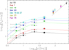 |
Fig. 6 Flux density measured from S255 NIRS 3 as a function of frequency (points). The curves represent the best fits to the different epochs obtained with the model by Reynolds (1986). Symbols with the same colour correspond to the same epoch, as explained in the figure. The black point at 225 GHz is the measurement by Zinchenko et al. (2012). The dashed line denotes the expected mm emission according to Eq. (4). The vertical error bars correspond to the calibration uncertainty, while the horizontal bars indicate the frequency ranges covered by the VLA correlator at the different bands. |
Best-fit parameters at each observing epoch.
4.2 Origin of the millimetre emission
Thanks to our model fit, we can also analyze the nature of the millimetre emission observed with NOEMA and ALMA. It is interesting to note (see Fig. 6) that the flux densities measured with ALMA at 86.2 and 98.2 GHz (cyan points; see Table 1) are comparable, within the errors, to the sum of the free–free emission from the jet measured at the same epoch (cyan curve), i.e. ~22 mJy, plus the dust contribution of 41 mJy at 86.2 GHz and 54 mJy at 98.2 GHz expected at these frequencies on the basis of Eq. (4) (dashed line). We conclude that the small flux increase observed at millimetre wavelengths with respect to the (extrapolated) pre-burst literature flux can be entirely due to the free–free emission from the radio jet and not to dust heating by the outburst.
This result differs from the (sub)mm brightening detected by Hunter et al. (2017) in a similar high-mass YSO (NGC 6334I-MM1), also undergoing a maser flare and, possibly, an accretion outburst. Such a lack of brightening in the (sub)mm regime is puzzling given the similarities between the two outbursts. However, in our case the increase in the bolometric luminosity was ~13 times less than for NGC 6334I-MM1, and S255 NIRS 3 appears to be less deeply embedded. These differences could justify a shorter timescale for the decay of the dust temperature in our object. Naïvely, we might expect that a burst of energy takes longer to be dissipated in a thick envelope than in a disk for one simple geometrical reason: the surface-to-volume ratio of a thin cylinder is much greater than that of a sphere with the same radius, thus making irradiation more effective in cooling the gas.
4.3 Timelag between the IR and radio bursts
As seen in Sect. 4.1, the distance from the star at which the radio jet becomes ionized must be r0 < 70 au. Such a small value of r0 implies a timescale t0 = 2 r0∕0 < 9 months for the ejected material travelling at 0 = 900 km s−1 to reach r0 and trigger the jet ionization. If the onset of the ejection episode coincides with the accretion outburst detected in the IR, t0 appears inconsistent with the observed time lag between the IR and the radio bursts, which is significantly longer (~13 months). However, it should be kept in mind that the brightening of the radio emission can be detected only when the intensity of the radio burst overcomes the pre-existent flux density. For this to happen, it is necessary for the jet to expand well beyond r0 and it is hence plausible that a few more months are needed, corresponding to a jet expansion of the order of a few 10 au. In conclusion, we believe that the 13-month lag that we observed is compatible with the value of r0 = 50 au adopted in our model.
A consequence of the observed time lag is that the radio burst is unlikely to be due to photoionization because in this case the burst should have been detected at the same time at both IR and radio wavelengths. In fact, the timescale to photoionize the gas can be estimated using Eqs. (5.6) and (7.7) in Dyson & Williams (1980). Assuming a density of ~ 6 × 108 cm−3 for the inner regions of the disk (see Zinchenko et al. 2015), we find a timescale of only ~2.3 h, much less than the 13-month time lag between the IR burst and the radio burst. While it is possible that the density is lower in the direction of the disk axis, it seems more likely that the radio burst is triggered mechanically rather than by a “flash” of light. This scenario is consistent with a low ionization degree of the ejected gas, as discussed later in Sect. 4.5.
4.4 Evolution of jet parameters
The fits to the observed spectra allow us to investigate the variation of the jet physical parameters with time. Figures 7a and b show the best-fit values of x0 Ṁ∕0 and θ0 as a function of time fromthe estimated beginning of the radio burst. The errors were computed by applying the method used by Lampton et al. (1976) to the expression of χ2 in Eq. (10), for two free parameters.
From Table 3 we see that at the beginning of the radio burst the jet is quite collimated and the ionized mass loss rate is lower, of the order of 10−6 M⊙ yr−1. Subsequently, we see a steady increase in θ0, which indicates that the jet is progressively widening, while the ejection rate of the ionized gas x0 Ṁ is increasing. This result might look surprising because, according to our ongoing monitoring at IR wavelengths, the peak of the IR light-curve lies between November and December 2015; therefore, the outburst in December 2016 should already be fading. However, a few considerations are in order.
First of all, we do not have a precise estimate of the ionized fraction x0 and can only set an upper limit (see Sect. 4.5). Therefore, the increase in x0 Ṁ does not necessarily correspond to an increase in the mass loss rate, Ṁ. Furthermore, a rise in x0 Ṁ can be explained bythe increase in θ0 because the ionized mass flux at r0, 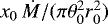 is constant within the errors, as shown in Fig. 8. Therefore, the augmented ejection rate of the ionized gas could be due to a widening of the ejection angle.
Finally,we actually do know that the radio burst occurred with a delay of ~13 months after the onset of the accretion burst and it is hence reasonable that the fading of the emission at the two bands also presents such a delay. This would imply that the radio intensity should begin to decrease at the beginning of 2017, ~13 months after the peak of the IR burst, which falls between December 2015 and January 2016 (Caratti o Garatti, priv. comm.). It is thus not surprising that the radio flux measured in December 2016 is still rising if the light curve of the radio burst mimicks the evolution of the accretion outburst with a delay of 13 months.
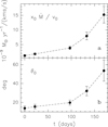 |
Fig. 7 Panel a: Best-fit parameter x0 Ṁ∕0 at the five observing epochs. The initial time, t = 0, corresponds to July 10, 2016. Panel b: Same as the previous panel, but for the other best-fit parameter θ0. |
 |
Fig. 8 Ionized mass flux through the radio jet at the five observing epochs. No significant change is observed within the errors. |
4.5 Weakly ionized jet
For the first time our study makes it possible to compute the ionization degree of a thermal jet, thanks to our knowledge of both the mass accretion rate and the ionized mass loss rate. Caratti o Garatti et al. (2017) have estimated an accretion rate of at least ~ 5 × 10⁻³ M⊙ yr−1 during the outburst. It is reasonable that at least 10% of the infalling material will be redirected into the outflow, so we can assume Ṁ > 10−4 M⊙ yr−1. From x0 Ṁ∕0 < 1.5 × 10⁻⁸ M⊙ yr−1∕(km s−1) (see Table 3) and 0 ≃ 900 km s−1, we obtain x0 Ṁ < 1.4 × 10⁻⁵ M⊙ yr−1 and x0 < 0.14. We note that this is a conservative upper limit. This result demonstrates that the ionized component is only a small fraction of the whole jet, which is mostly neutral.
Indeed, comparison with other studies strongly suggests that a low degree of ionization could be a common feature of all radio jets. For example, Guzmán et al. (2010), Purser et al. (2016), and Sanna et al. (2016) find ionized mass loss rates ranging from 2 × 10⁻⁷ to 8 × 10⁻⁶ M⊙ yr−1, values even lower than that estimated by us for S255 NIRS 3. In conclusion, our results demonstrate that the ionized component of the jet is dynamically negligible.
Finally, we note that a jet with a low ionization fraction is clearly different from the fully ionized bubbles predicted by Tanaka et al. (2016). Since in their case the gas is photoionized, our finding further supports the idea that in S255 NIRS 3 we are observing a thermal jet. In turn, the lack of an HII region around a (proto)star as massive as S255 NIRS 3 (~20 M⊙; Zinchenko et al. 2015) suggests that such a region could be quenched, consistent with the large accretion rate estimated in our case (see Yorke 1986; Walmsley 1995). In addition, we could be dealing with a bloated, colder protostar, whose Lyman continuum emission is much less than that expected for a zero-age main-sequence star with the same mass (see Hosokawa et al. 2010).
5 Summary and conclusions
We have reported on the first detection of a radio burst in a massive YSO (S255 NIRS 3) that had previously undergone an accretion outburst revealed in the methanol maser and IR emission. Along with methanol maser flares, IR and mm flux variability, the radio variability from thermal jets can thus be considered an additional signpost of accretion bursts in high-mass YSOs, especially for deeply embedded objects where even the near-IR emission can be heavily extincted.
The structure of the radio source seen in archival VLA maps prior to the burst is strongly suggestive of a bipolar thermal jet, with two lobes extending NE and SW. The burst is observed only towards the central, unresolved radio source presumably coinciding with the YSO.
The analysis of the first six epochs of our on-going monitoring in the range 6–46 GHz indicates that the radio burst started right after July 10, 2016, and that the flux density at all frequencies was still increasing exponentially until December 2016. We measure a time lag of ~13 months between the beginning of the IR outburst and that of the radio burst.
At the last epoch we detect a barely resolved elongation to the NE in the direction of the jet axis, which we interpret as an expanding lobe of the ionized gas powered by the outburst.
In order to reproduce the observed flux variations, we adopted the model developed by Reynolds (1986) under simplifying assumptions. In particular, we assume that the jet is initially accelerated up to a distance r0 where it becomes ionized. We infer r0 ≃ 50 au. Beyond this distance the jet expands at constant speed. We obtain the best fit to the observed spectra at the last five epochs by varying onlytwo parameters: the opening angle of the jet and the ratio between the ionized mass loss rate and the expansion speed.
Our best fits indicate that both parameters increase with time during the burst, while the mass flux of the ionized gas through the jet remains roughly constant. This suggests that the increase in the ionized mass loss rate could be due to widening of the jet opening angle.
Finally, by comparison between the accretion rate computed from the IR outburst (Caratti o Garatti et al. 2017) and the ionized mass loss rate of the jet, we estimate for the first time the ionization fraction in the jet and find a conservative upper limit of 14%. This result strongly indicates that the radio emission from thermal jets very likely traces only a negligible fraction of the jet mass, which is largely neutral.
Acknowledgements
It is a pleasure to thank Francesca Bacciotti for stimulating discussions on jets from YSOs. We also thank the Italian ARC node and the IRAM technical staff for their support in this project. The research leading to these results has received funding from the European Unions Horizon 2020 research and innovation programme under grant agreement No. 730562 [RadioNet]. This study is based on observations made under the project 16A-424 of the VLA of NRAO. The National Radio Astronomy Observatory is a facility of the National Science Foundation operated under cooperative agreement by AssociatedUniversities, Inc. This work is also based on observations carried out under project number E16AB with the IRAM NOEMA Interferometer. IRAM is supported by INSU/CNRS (France), MPG (Germany), and IGN (Spain). This paper makes use of the following ALMA data: ADS/JAO.ALMA#2016.A.00008.T. ALMA is a partnership of ESO (representing its member states), NSF (USA), and NINS (Japan), together with NRC (Canada), NSC and ASIAA (Taiwan), and KASI (Republic ofKorea), in cooperation with the Republic of Chile. The Joint ALMA Observatory is operated by ESO, AUI/NRAO, and NAOJ. A. C. G. and T. P. R. have received funding from the European Research Council (ERC) under the European Union’s Horizon 2020 research and innovation programme (grant agreement No. 743029).
Appendix A Turn-over frequencies of thermal jet spectra
We want to determine the relation between the turn-over frequencies of a typical thermal jet spectrum and the minimum (r0) and maximum (rmax) radius of the jet itself. Our derivation is based on the model by Reynolds (1986).
In Fig. A.1 we show a schematic spectrum of a radio jet. We can identify three regimes separated by the two turn-over frequencies that we denote νm (following Reynolds’ notation) and νt. Since the free–free opacity decreases with frequency, there must be a sufficiently low frequency, νt, below which the whole jet (i.e. between r0 and rmax) is optically thick. The spectrum in this regime is characterized by the power law ∝ ν2, typical of optically thick free–free emission. Conversely, for a sufficiently high frequency above νm, the whole jet becomes optically thin and the power law becomes ∝ ν−0.1. Between νt and νm the flux density is contributed by both optically thick and thin emission, and Reynolds demonstrates that the slope takes the value of ~0.6 in the simple case of a conical, isothermal jet with density scaling ∝ r−2 (see his Table 1).
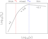 |
Fig. A.1 Schematic radio continuum spectrum of a typical thermal jet. The two turn-over frequencies at the border of the optically thick and thin regions of the spectrum are indicated at the top of the figure. The regime between the two frequencies is characterized by a mixture of thin and thick emission. The numbers indicate the slopes in the three parts of the spectrum; 0.6 refers to the simple case adopted by us. |
The value of νm is obtained by Reynolds in his Eq. (13) from the condition r1 = r0, where r1 is the radius at which the free–free opacity equals 1. This assumes that the optical depth decreases with increasing r, as expected if the density of the ionized gas also decreases.
Taking into account Reynolds’ expression for Ṁ, we can rewrite Reynolds’ Eq. (13) in a more convenient form for our purposes,
![Mathematical equation: \begin{equation*} \nu_{\textrm{m}} = \left[ \frac{2\,a_{\kappa}}{(\pi \mu)^2} \, (\theta_0\,r_0)^{-3} \, \left(\frac{x_0 \dot{M}}{\varv_0}\right)^2 T_0^{-1.35} \, (\sin i)^{-1} \right]^{\frac{1}{2.1}},\end{equation*}](/articles/aa/full_html/2018/04/aa32238-17/aa32238-17-eq17.png) (A.1)
(A.1)
where the symbols are the same as in Sect. 4.
The value of νt can be computed in a similar way, from the condition r1 = rmax. Taking into account that y = r sini and using Reynolds’ Eq. (12), this condition can be written as
![Mathematical equation: \begin{equation*} \left[ \frac{2\,a_{\kappa}}{(\pi \mu)^2}\, (\theta_0 \,r_0)^{-3} \left(\frac{x_0 \dot{M}}{\varv_0}\right)^2\! T_0^{-1.35} (\sin i)^{-1} \, r_0^{-q_{\tau}} \nu_t^{-2.1} \right]^{-\frac{1}{q_{\tau}}} = r_{\textrm{max}} ,\end{equation*}](/articles/aa/full_html/2018/04/aa32238-17/aa32238-17-eq18.png) (A.2)
(A.2)
where qτ is given by Reynolds’ Eq. (6). From this, we have
![Mathematical equation: \begin{equation*} \nu_{\textrm{t}} = \left[ \!\frac{2a_{\kappa}}{(\pi \mu)^2} \, (\theta_0 \,r_0)^{-3} \left(\!\frac{x_0 \dot{M}}{\varv_0}\right)^2\! T_0^{-1.35} \, (\sin i)^{-1} \left(\frac{r_0}{r_{\textrm{max}}}\right)^{-q_{\tau}} \right]^{\frac{1}{2.1}}.\end{equation*}](/articles/aa/full_html/2018/04/aa32238-17/aa32238-17-eq19.png) (A.3)
(A.3)
Finally, from Eqs. (A.1) and (A.3) we obtain
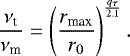 (A.4)
(A.4)
In conclusion, for a given value of qτ, the ratio between the two turn-over frequencies depends only on the ratio between the outer and inner radius of the jet, and vice versa. The case considered in our study corresponds to qτ = −3 (see Reynolds’ Table 1), hence
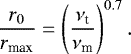 (A.5)
(A.5)
References
- Acosta-Pulido,J. A., Kun, M., Ábrahám, P., et al. 2007, AJ, 133, 2020 [NASA ADS] [CrossRef] [Google Scholar]
- Audard, M., Ábrahám, P., Dunham, M. M., et al. 2014, in Protostars and Planets VI, eds. H. Beuther, R. S. Klessen, C. P. Dullemond, & T. Henning, (Tucson: Univ. of Arizona Press), 387 [Google Scholar]
- Boley, P. A., Linz, H., van Boekel, R., et al. 2013, A&A, 558, A24 [NASA ADS] [CrossRef] [EDP Sciences] [Google Scholar]
- Burns, R. A., Handa, T., Nagayama, T., Sunada, K., & Omodaka, T. 2016, MNRAS, 460, 283 [NASA ADS] [CrossRef] [Google Scholar]
- Caratti o Garatti, A., Garcia Lopez, R., Scholz, A., et al. 2011, A&A, 526, L1 [NASA ADS] [CrossRef] [EDP Sciences] [Google Scholar]
- Caratti o Garatti, A., Garcia Lopez, R., Weigelt, G., et al. 2013, A&A, 554, A66 [NASA ADS] [CrossRef] [EDP Sciences] [Google Scholar]
- Caratti o Garatti, A., Stecklum, B., Garcia Lopez, R., et al. 2017, Nat. Phys., 13, 276 [NASA ADS] [CrossRef] [Google Scholar]
- Cesaroni, R., Massi, F., Arcidiacono, C., et al. 2013, A&A, 549, A146 [NASA ADS] [CrossRef] [EDP Sciences] [Google Scholar]
- Contreras Peña, C., Lucas, P. W., Kurtev, R., et al. 2017, MNRAS, 465, 3039 [NASA ADS] [CrossRef] [Google Scholar]
- Dyson, J. E., & Williams, D. A. 1980, The Physics of the Interstellar Medium (Manchester: Manchester University Press) [Google Scholar]
- Fujisawa, K., Yonekura, Y., Sugiyama, K., et al. 2015, ATel, 8286, 1 [NASA ADS] [Google Scholar]
- Guzmán, A. E., Garay, G., & Brooks, K. J. 2010, ApJ, 725, 734 [NASA ADS] [CrossRef] [Google Scholar]
- Hosokawa, T., Yorke, H. W., & Omukai, K. 2010, ApJ, 721, 478 [NASA ADS] [CrossRef] [Google Scholar]
- Hunter, T. R., Brogan, C. L., MacLeod, G., et al. 2017, ApJ, 837, L29 [NASA ADS] [CrossRef] [Google Scholar]
- Krumholz, M. R., Klein, R. I., & McKee, C. F., 2007, ApJ, 656, 959 [NASA ADS] [CrossRef] [Google Scholar]
- Kuiper, R., Klahr, H., Beuther, H., & Henning, Th. 2010, ApJ, 722, 1556 [CrossRef] [Google Scholar]
- Lampton, M., Margon, B., & Bowyer, S. 1976, ApJ, 208, 177 [NASA ADS] [CrossRef] [Google Scholar]
- Melnikov, S. Y., Woitas, J., Eislffel, J., et al. 2008, A&A, 483, 199 [NASA ADS] [CrossRef] [EDP Sciences] [Google Scholar]
- Melnikov, S. Y., Eislffel, J., Bacciotti, F., Woitas, J., & Ray, T. P. 2009, A&A, 506, 763 [NASA ADS] [CrossRef] [EDP Sciences] [Google Scholar]
- Moscadelli, L., Sanna, A., Goddi, C., et al. 2017, A&A, 600, L8 [NASA ADS] [CrossRef] [EDP Sciences] [Google Scholar]
- Peters, T., Banerjee, R., Klessen, R. S., et al. 2010, ApJ, 711, 1017 [NASA ADS] [CrossRef] [Google Scholar]
- Pudritz, R. E., Ouyed, R., Fendt, Ch., & Brandenburg, A. 2007, in Protostars and Planets V, eds. B. Reipurth, D. Jewitt, & K. Keil (Tucson: Univ. of Arizona Press), 277 [Google Scholar]
- Purser, S. J. D., Lumsden, S. L., Hoare, M. G., et al. 2016, MNRAS, 460, 1039 [NASA ADS] [CrossRef] [Google Scholar]
- Reynolds, S. P. 1986, ApJ, 304, 713 [NASA ADS] [CrossRef] [Google Scholar]
- Sánchez-Monge, Á., Schilke, P., Ginzburg, A., Cesaroni, R., & Schmiedeke, A. 2018, A&A, 609, A101 [NASA ADS] [CrossRef] [EDP Sciences] [Google Scholar]
- Sanna, A., Moscadelli, L., Cesaroni, R., et al. 2016, A&A, 596, L2 [NASA ADS] [CrossRef] [EDP Sciences] [Google Scholar]
- Stecklum, B., Caratti o Garatti, A., Cardenas, M. C., et al. 2016, ATel, 8732, 1 [NASA ADS] [Google Scholar]
- Tanaka, K. E. I., Tan, J. C., & Zhang, Y. 2016, ApJ, 818, 52 [NASA ADS] [CrossRef] [Google Scholar]
- Tapia, M., Roth, M., & Persi, P. 2015, MNRAS, 446, 4088 [NASA ADS] [CrossRef] [Google Scholar]
- Walmsley, M. 1995, in Circumstellar Disks, Outflows, and Star Formation, eds. S. Lizano, & J. M. Torrelles (Mexico, DF: Inst. Astron., UNAM), Rev. Mex. Astron. Astrofis. Ser. Conf., 1, 137 [Google Scholar]
- Wang, Y., Beuther, H., Bik, A., et al. 2011, A&A, 527, A32 [NASA ADS] [CrossRef] [EDP Sciences] [Google Scholar]
- Yorke, H. 1986, ARA&A, 24, 49 [NASA ADS] [CrossRef] [Google Scholar]
- Zinchenko, I., Liu, S.-Y., Su, Y.-N., et al. 2012, ApJ, 755, 177 [NASA ADS] [CrossRef] [Google Scholar]
- Zinchenko, I., Liu, S.-Y., Su, Y.-N., et al. 2015, ApJ, 810, 10 [NASA ADS] [CrossRef] [Google Scholar]
The Common Astronomy Software Applications software can be downloaded at http://casa.nrao.edu
The GILDAS software has been developed at IRAM and Observatoire de Grenoble: http://www.iram.fr/IRAMFR/GILDAS
A different spectral index, e.g. 4, does not change the estimate of α significantly.
Reynolds’ Eq. (8) takes into account emission from only one lobe of the jet, whereas we assume the jet to be bipolar and multiply the flux by a factor of 2 to take both lobes into account.
All Tables
Flux densities measured towards the central core of S255 NIRS 3 with the VLA, IRAM/NOEMA, and ALMA at different epochs, and corresponding mean synthesized beams.
Flux densities measured at mm wavelengths towards S255 NIRS 3 with the SMA by various authors.
All Figures
|
Fig. 1 Panel a: VLA archival image obtained on August 27, 1990, at 3.6 cm with the C-array configuration. The values of the contour levels are drawn in the corresponding colour scales to the right. The full width at half power of the synthesized beam is shown in the bottom right. Panel b: Same as the top panel, after smoothing to the resolution of our new 3 cm image. Panel c: Same as the other panels, but for our new 3 cm image obtained on March 11, 2016, with the C-array configuration. The bipolar structure of the jet is shown, consisting of a central core associated with NIRS 3 and two main knots to theNE and SW. |
| In the text | |
|
Fig. 2 Maps of the S255 NIRS 3 region at centimetre wavelengths obtained with the VLA on July 10 (left panels) and August 1 (right panels), 2016. The offsets are computed with respect to the phase centre of the observations, i.e. 06h 12m 54. s02, 17°59′23.′′1. The corresponding synthesized beams are shown at the bottom right of each panel. The values of the contour levels are marked in the colour scales to the right, and in all cases the lowest contour is >4σ. We note thebrightening of NIRS 3 at all frequencies. |
| In the text | |
|
Fig. 3 Observed radio flux densities of NIRS 3 as a function of time, with t = 0 corresponding to the second epoch of our monitoring (July 10, 2016). The solid lines connect fluxes observed at the same frequency, which is given beside each curve. The dashed lines are the fits assuming exponential dependence on t according to Eq. (1). |
| In the text | |
|
Fig. 4 Continuum map at 22.2 GHz of the radio source NIRS 3 obtained at the fifth epoch of our monitoring (December 27, 2016). The image has been saturated to emphasize the elongated structure. The dashed line denotes thedirection connecting NIRS 3 to the NE knot of the large-scale radio jet. Contour levels range from 0.6 (7σ) to 13.2 in steps of 1.8 mJy/beam. The ellipse in the bottom left denotes the synthesized beam. |
| In the text | |
|
Fig. 5 Panel a: Flux densities at 225 GHz and 230 GHz from Table 2 versus the full width at half power of the corresponding synthesized beam. The 230 GHz flux (empty point) has been scaled to 225 GHz (solid point) assuming Sν ∝ ν2. The straight line is the linear fit (in the logarithmic plot) to the solid points, based on Eq. (3). Panel b: Flux densities from Table 2 as a function of frequency before (empty points) and after (solid points) scaling the fluxes to an angular resolution of 3.′′ 37 (see text) with Eq. (3). The straight line is the linear fit (in the logarithmic plot) to the solid points, based on Eq. (4). |
| In the text | |
|
Fig. 6 Flux density measured from S255 NIRS 3 as a function of frequency (points). The curves represent the best fits to the different epochs obtained with the model by Reynolds (1986). Symbols with the same colour correspond to the same epoch, as explained in the figure. The black point at 225 GHz is the measurement by Zinchenko et al. (2012). The dashed line denotes the expected mm emission according to Eq. (4). The vertical error bars correspond to the calibration uncertainty, while the horizontal bars indicate the frequency ranges covered by the VLA correlator at the different bands. |
| In the text | |
|
Fig. 7 Panel a: Best-fit parameter x0 Ṁ∕0 at the five observing epochs. The initial time, t = 0, corresponds to July 10, 2016. Panel b: Same as the previous panel, but for the other best-fit parameter θ0. |
| In the text | |
|
Fig. 8 Ionized mass flux through the radio jet at the five observing epochs. No significant change is observed within the errors. |
| In the text | |
|
Fig. A.1 Schematic radio continuum spectrum of a typical thermal jet. The two turn-over frequencies at the border of the optically thick and thin regions of the spectrum are indicated at the top of the figure. The regime between the two frequencies is characterized by a mixture of thin and thick emission. The numbers indicate the slopes in the three parts of the spectrum; 0.6 refers to the simple case adopted by us. |
| In the text | |
Current usage metrics show cumulative count of Article Views (full-text article views including HTML views, PDF and ePub downloads, according to the available data) and Abstracts Views on Vision4Press platform.
Data correspond to usage on the plateform after 2015. The current usage metrics is available 48-96 hours after online publication and is updated daily on week days.
Initial download of the metrics may take a while.