| Issue |
A&A
Volume 612, April 2018
|
|
|---|---|---|
| Article Number | A18 | |
| Number of page(s) | 11 | |
| Section | Extragalactic astronomy | |
| DOI | https://doi.org/10.1051/0004-6361/201732162 | |
| Published online | 10 April 2018 | |
Anatomy of the AGN in NGC 5548
IX. Photoionized emission features in the soft X-ray spectra
1
SRON Netherlands Institute for Space Research,
Sorbonnelaan 2,
3584 CA
Utrecht, The Netherlands
e-mail: J.Mao@sron.nl
2
Leiden Observatory, Leiden University,
Niels Bohrweg 2,
2300 RA
Leiden, The Netherlands
3
RIKEN Nishina Center,
2-1 Hirosawa,
Wako,
Saitama
351-0198, Japan
4
Space Telescope Science Institute,
3700 San Martin Drive,
Baltimore,
MD
21218, USA
5
Dipartimento di Matematica e Fisica, Università degli Studi Roma Tre,
via della Vasca Navale 84,
00146
Roma, Italy
6
Mullard Space Science Laboratory, University College London,
Holmbury St. Mary,
Dorking,
Surrey
RH5 6NT, UK
7
Department of Physics, Technion-Israel Institute of Technology,
32000
Haifa, Israel
8
Department of Astronomy, University of Geneva,
16 Ch. d’Ecogia,
1290
Versoix, Switzerland
9
Univ. Grenoble Alpes, IPAG,
38000
Grenoble, France
10
CNRS, IPAG,
38000
Grenoble, France
11
European Space Astronomy Centre,
PO Box 78,
28691
Villanueva de la Cañada, Madrid, Spain
12
Max Planck Institute fur Extraterrestriche Physik,
85748
Garching, Germany
Received:
24
October
2017
Accepted:
20
December
2017
The X-ray narrow emission line region (NELR) of the archetypal Seyfert 1 galaxy NGC 5548 has been interpreted as a single-phase photoionized plasma that is absorbed by some of the warm absorber components. This scenario requires those overlaying warm absorber components to have larger distance (to the central engine) than the X-ray NELR, which is not fully consistent with the distance estimates found in the literature. Therefore, we reanalyze the high-resolution spectra obtained in 2013–2014 with the Reflection Grating Spectrometer (RGS) aboard XMM-Newton to provide an alternative interpretation of the X-ray narrow emission features. We find that the X-ray narrow emission features in NGC 5548 can be described by a two-phase photoionized plasma with different ionization parameters (logξ = 1.3 and 0.1) and kinematics (vout = −50 and −400 km s−1), and no further absorption by the warm absorber components. The X-ray and optical NELR might be the same multi-phase photoionized plasma. Both X-ray and optical NELR have comparable distances, asymmetric line profiles, and the underlying photoionized plasma is turbulent and compact in size. The X-ray NELR is not the counterpart of the UV/X-ray absorber outside the line of sight because their distances and kinematics are not consistent. In addition, X-ray broad emission features that we find in the spectrum can be accounted for by a third photoionized emission component. The RGS spectrum obtained in 2016 is analyzed as well, where the luminosity of most prominent emission lines (the O VII forbidden line and O VIII Lyα line) are the same (at a 1σ confidence level) as in 2013–2014.
Key words: X-rays: galaxies / galaxies: active / galaxies: Seyfert / galaxies: individual: NGC 5548 / techniques: spectroscopic
© ESO 2018
1 Introduction
Two types of emission lines are commonly observed in the optical spectra of active galactic nuclei (AGN): broad emission lines with a velocity broadening of a few 103 km s−1 and narrow emission lines with a velocity broadening of a few 102 km s−1. The optical broad and narrow emission lines stem from the so-called broad and narrow emission line regions (BELR and NELR, see Netzer 2015, for a recent review), with the former closer (a few light days to weeks, Peterson et al. 2004) to the central engine and the latter further away (at least a few parsecs, Bennert et al. 2006a,b).
In the X-ray band, broad and narrow emission lines are also observed (e.g., Kaastra et al. 2000; Steenbrugge et al. 2005; Costantini et al. 2007, 2016), often along with the characteristic narrow radiative recombination continua (RRC) of a photoionized plasma. The spatial extent and overall morphology of the optical and the X-ray NELRs are remarkably similar in a small sample of nearby Seyfert 2 galaxies (Bianchi et al. 2006). Nonetheless, there is no conclusive evidence that the optical and X-ray narrow emission features originate from the same photoionized plasma with a multi-phase nature.
In terms of detailed spectral modeling of the narrow emission features in the X-ray band, a two-step approach is commonly used. First, a phenomenological local fit (e.g., Guainazzi & Bianchi 2007) is performed for individual emission lines and RRC. Typically, the (local) continuum is simply modeled as a (local) power law or spline function plus a model for RRC and an emission line is modeled with a Gaussian or delta profile. The local fit is straightforward and useful, providing primary information like whether a single line is shifted and/or broadened, the temperature of a photoionized plasma (via the width of the RRC), the temperature and density of the plasma (via the line ratios of the He-like triplets), etc.
With the knowledge obtained from the local fit, the entire spectrum is then modeled with a self-consistent plasma model, or a combination of plasma models (e.g. Guainazzi et al. 2009). The plasma model can be a photoionized plasma either with a single photoionized component (e.g., Whewell et al. 2015) or multiple photoionized components (e.g., Kinkhabwala et al. 2002; Armentrout et al. 2007; Longinotti et al. 2008; Nucita et al. 2010; Marinucci et al. 2011; Kallman et al. 2014), and sometimes a collisional ionized equilibrium (CIE) plasma, which is associated to star formation (Guainazzi et al. 2009) or jets (Bianchi et al. 2010).
For the photoionized plasma modeling, the widely used approach is to simulate a set of photoionized spectra with the Cloudy code (Ferland et al. 2017) for a fixed ionizing spectral energy distribution (SED) and for a grid of physical parameters, including the ionization parameter, the line of sight column density and sometimes the plasma number density and microscopic turbulence velocity as well. The number of free parameters and the size of the grid are limited, otherwise, it is computationally too expensive to simulate. Subsequently, the observed spectra are compared with these pre-calculated models, with the best-fit of the physical parameters derived from the closest match. This last step is carried out in a separate spectral fitting package, e.g. XSPEC (Arnaud 1996).
A different approach for the photoionized plasma modeling is used here (see also Mao et al. 2017). We use SPEX (v3.03.02 Kaastra et al. 1996) to fit the entire observed spectra on the fly. The advantage of the SPEX code is that it includes an extensive atomic database and self-consistent plasma models, e.g. PION1 for the photoionized plasma, which utilizes the state-of-the-art atomic data (Kaastra et al. 2017). We refer to Mehdipour et al. (2016b) for a detailed comparison of the photoionization calculation between SPEX, Cloudy and XSTAR (Kallman & Bautista 2001; Bautista & Kallman 2001). In each step of the photoionized plasma fitting, the intrinsic SED, thermal equilibrium, ionization balance, level population, transmission, emissivity, and line broadening are calculated in real time to account for the absorption and emission features self-consistently. In short, the photoionization calculation is consistent with the instant ionizing SED and without pre-calculations using grid-defined parameters, thus, more freedom and higher consistency can be achieved in SPEX.
NGC 5548 is the archetypal Seyfert 1 galaxy, with broad and narrow emission features across its optical to X-ray spectra (e.g. Korista et al. 1995; Chiang et al. 2000; Peterson et al. 2002; Kaastra et al. 2002; Steenbrugge et al. 2005). The extensive multi-wavelength campaign of NGC 5548 in 2013–2014 (Kaastra et al. 2014; Mehdipour et al. 2015) unveiled a special state of the source, where the soft X-ray flux is highly obscured. Such a special state offers a unique opportunity to study the narrow emission lines and radiative recombination continua that were previously hidden by the unobscured continuum (Kaastra et al. 2002; Steenbrugge et al. 2005; Detmers et al. 2009). With a detailed study of the narrow emission features using both the local fit and Cloudy based photoionization modeling, Whewell et al. (2015) interpret the X-ray NELR as a single-phase photoionized plasma that is absorbed by the warm absorber components B+E or A+B+C (see Table S2 of Kaastra et al. 2014, for the nomenclature). That is to say, these warm absorber components intervene along the line of sight from the X-ray narrow line emitter to the observer.
This scenario does not fully agree with the distance estimates of the X-ray NELR and warm absorber components in NGC 5548. Using the variability of the forbidden line of O VII, Detmers et al. (2009) derived a distance of 1–15 pc for the X-ray NELR, consistent with the optical NELR distance estimate of 1–3 pc (Peterson et al. 2013) and joint optical and X-ray NELR distance estimate of ~ 2.4 pc (Landt et al. 2015). According to the Cloudy based photoionization modeling, Whewell et al. (2015) found that the X-ray narrow emission lines originate mainly from the illuminated face of the X-ray NELR with a distance of 14 pc. Ebrero et al. (2016) estimate the distance of the warm absorber components based on variability, with component A and B at least 10 pc away from the central engine and components C to F within 5 pc from the central engine. Nonetheless, based on a spectral analysis using the density sensitive metastable absorption lines, Mao et al. (2017) found the warm absorber component B is even closer (<0.23 pc, 3σ upper limit) than the optical NELR, rather than further away. Ebrero et al. (2016) constrain the lower limit of the distance of the warm absorber component B based on the non-detection of variability on a timescale of 500 days. However, the authors also pointed out that there are marginal hints of variability at 4 and 60 days. If the variability at a shorter timescale is true, the inferred distance of component B would be much smaller.
Therefore, we reanalyze the high-resolution spectra of NGC 5548 obtained with the Reflection Grating Spectrometer (RGS; den Herder et al. 2001) aboard XMM-Newton (Jansen et al. 2001) to provide an alternative interpretation of the X-ray narrow emission features. To be more specific, we attempt to model the soft X-ray emission features with a multi-phase photoionized plasma with no additional absorption by the warm absorber components. Whewell et al. (2015) did not consider this scenario in their study.
In Sect. 2, we present the observed RGS spectrum. We describe the detailed spectral analysis in Sect. 3, including the phenomenological local fit (Sect. 3.1) and the physical global fit (Sect. 3.2). The physical global fit is based on the self-consistent photoionization model PION in the SPEX code, with both the single-phase and multi-phase scenarios studied. We discuss the relation between the X-ray and optical narrow emission line region in Sect. 4.1 and the relation between the X-ray emitter and absorber in Sect. 4.2, respectively. We justify our usage of the unobscured ionizing SED for the X-ray emitter in Sect. 4.3. We also point out the abnormally high Lyγ/Lyα ratio of N VII and discuss it in terms of a possible charge exchange component in Sect. 4.4. The summary can be found in Sect. 5.
2 Observations and data reduction
The RGS data used here are obtained in two epochs, June 2013 – February 2014 (PI: J. Kaastra) and January 2016 (PI: G. Kriss), respectively. Data for the first epoch (2013–2014) are taken as part of a large multi-wavelength campaign ofNGC 5548 (Kaastra et al. 2014). There are in total fourteen XMM-Newton observations (~50 ks exposure each), where twelve of them are taken between 22 June and 31 July 2013 and the last two are taken in December 2013 and February 2014, respectively. The observation log of 2013–2014 can be found in Mehdipour et al. (2015, their Table 1) and Table 1 lists the observation log for 2016.
Details of the RGS data reduction method are similar to those described in Kaastra et al. (2011). The first-order RGS1 and RGS2 spectra for all observations are stacked for each epoch, with a total exposure of ~770 ks (for 2013–2014) and ~70 ks (for 2016), respectively. The stacked RGS spectrum of 2013–2014 is the same one as that used by Whewell et al. (2015) for the study of thenarrow emission features.
The observation log of NGC 5548 in 2016 (PI: G. Kriss) with XMM-Newton.
3 Spectral analysis and results
SPEX v3.03.02 is used for the spectral analysis. We use the C-statistic throughout this work (Kaastra 2017). Statistical errors are quoted at 68% confidence level (Δ C = 1.0), unless indicated otherwise. The spectral fit is performed in the 7–35 Å wavelength range. Both stacked 2013–2014 and 2016 spectra are optimally binned (Kaastra & Bleeker 2016) for the following spectral analysis (Sect. 3). The redshift of the AGN is fixed to z = 0.017175 (de Vaucouleurs et al. 1991), as given in the NASA/IPAC Extragalactic Database (NED).
3.1 The phenomenological local fit
In order to check the variability of the narrow emission features between 2013–2014 and 2016, we perform a simple local fit to spectra from the two epochs with a spline continuum model (SPLN in SPEX, see also Detmers et al. 2008), Gaussian line models (GAUS) and radiative recombination continua (RRC).
Even in the 770 ks 2013–2014 spectrum, the X-ray broad emission lines are difficult to fit due to their low significance (Whewell et al. 2015). Therefore, in this exercise, we do not include them in both spectra. In the 2016 spectrum, the Lyα line of O VIII and the forbidden line of O VII can be relatively well constrained, with statistical uncertainties ≲ 20%. The rest of the lines and RRC tabulated in Table 2 have statistical uncertainties between 30% to 100% in the 2016 spectrum. In Table 2, we compare the intrinsic (unabsorbed) luminosity of these lines and RRC between the two epochs.
The most prominent narrow emission lines (the O VIII Lyα and O VII forbidden lines) have remained constant (at a 1σ confidence level) in the two epochs June 2013 – February 2014 and January 2016. This is not totally unexpected,as shown in Table 2 of Detmers et al. (2009), the O VII line flux is also consistent within 1σ for two epochs on a similar timescale, December 1999 – February 2000 and January 2002.
On the other hand, some weak features might have varied by a factor of two (the Ne ix RRC and N vi forbidden line), but still within a 2σ confidence level.
The intrinsic (unabsorbed) luminosity of the prominent narrow emission features for the 2013–2014 and 2016 RGS spectra of NGC 5548.
3.2 The physical global fit
For the physical global fit (Sect. 3.2), we first model the high-quality 2013–2014 spectrum with different models (Sect. 3.2.1). Then we simply apply the best-fit model to the low-quality 2016 spectrum (Sect. 3.2.2).
Our global fit includes the following components: (1) the intrinsic broadband spectral energy distribution (SED) of the AGN; (2) the Galactic absorption; (3) the continuum absorption caused by the obscurer; (4) the absorption features caused by the warm absorber; (5) the narrow and/or broad emission features caused by the X-ray emitter.
The intrinsic SED consists of a Comptonized disk component (COMT in SPEX, for optical to soft X-ray), a power-law component (POW for X-ray), and a reflection component (REFL for the Fe K line and hard X-ray). For the 2013–2014 spectral analysis, all the relevant parameters are fixed to those values given in Mehdipour et al. (2015), where the best constraints on these parameters have been obtained from multi-wavelength data. For the 2016 spectral analysis, we fixed the parameters in the COMT component to values that corresponds to the average UVW2 flux in 2016 (the correlations can be found in Mehdipour et al. 2016a). The power-law and reflection components are allowed to vary in order to match the EPIC-pn data.
The Galactic absorption with NH = 1.45 × 1024 m−2 (Wakker et al. 2011) is modeled with the collisional ionisation equilibrium absorption model (HOT) (de Plaa et al. 2004; Steenbrugge et al. 2005) in SPEX. The electron temperature of the HOT component is fixed to 0.5 eV to mimic the transmission of a neutral gas.
The continuum absorption caused by the obscurer is modeled with two XABS components (Kaastra et al. 2014; Mehdipour et al. 2017). The line of sight (LOS) hydrogen column densities (NH ) and absorption covering factors (fcov) are allowed to vary in both 2013–2014 and 2016 spectra. The ionization parameters of the two XABS components are treated differently, with the warmer one allowed to vary (logξ ~−1) and the cooler one fixed to −4 (Di Gesu et al. 2015).
The absorption features caused by the warm absorber are accounted for using six PION components. In both the 2013–2014 and 2016 spectra, the hydrogen column densities (NH ), outflow velocities (vout ), and microscopic turbulence velocities (vmic) of the PION components are fixed to values given in Mao et al. (2017), which are obtained by fitting the high quality 2002 Chandra grating spectra of NGC 5548. Nonetheless, the ionization parameters (log ξ) can differ for these three epochs, due to the variability of the obscurer, as well as the changes of the intrinsic SED (Cappi et al. 2016). The ionization parameters are assumed to be proportional to the 1–103 Ryd ionizing luminosity. That is to say, the number density times distance squared (nH r2) in the later two epochs is assumed to be the same as in 2002.
The narrow and broad emission features caused by the X-ray emitter (sometimes called the warm mirror) are also modeled with PION. Six free parameters of each emission PION component are allowed to vary, including the hydrogen column densities (NH ), ionization parameters (log ξ), outflow velocities (vout ), and turbulence velocities (vmic) and the emission covering factors (Ccov, see next paragraph). Additionally, each emission PION component is convolved with a Gaussian velocity broadening model (VGAU in SPEX), with the velocity parameter (vmac) free to vary, to account for macroscopic motion.
Note that there are two covering factors in the PION model. The absorption covering factor fcov is used to model any partial covering in the line of sight (similar to that of the XABS component). The emission covering factor, Ccov= Ω∕4π, corresponds to the normalized solid angle sustained by the emitting region as seen from the central engine. In our modeling, each absorption PION component has fixed fcov = 1 and Ccov= 0, while each emission PION component has fixed fcov = 0 and free Ccov ∈ (0, 1). Furthermore, the ionizing SED for the absorption PION components is the obscured SED, as the obscurer locates between the warm absorber and the central engine (Kaastra et al. 2014). Nevertheless, the ionizing SED received by the emission PION components is assumed to be unobscured, and we will discuss this in detail in Sect. 4.3. Unless indicated otherwise, the proto-solar abundances of Lodders et al. (2009) are used for all plasma models (HOT, XABS and PION).
3.2.1 The 2013–2014 RGS spectrum
Five different models are used for the emission features in the RGS band. We start with a single-phase photoionized emitter (denoted as Model S0), which can reproduce well some of the observed narrow emission features, but not all. In particular, Model S0 fails to match the RRC of O VII (~17 Å) and C vi (~32 Å), the forbidden lines of N vi (~30 Å), etc. The fit residuals can be found the in top panels in Figs. 2 and 3. The residuals indicate that either additional absorption is required or the X-ray emitter has at least two emission components.
Following Whewell et al. (2015), we apply absorption caused by the warm absorber components B+E (Model S1) or A+B+C (Model S2) to the single-phase photoionized emitter. As expected, for both models, the C-stat is significantly improved (Table 3). Model S2 yields more consistent parameters with Whewell et al. (2015), i.e. a mildly ionized (log ξ ~ 1 − 1.5), blueshifted (vout ~−300 km s−1), turbulent (vmic ~ 200 km s−1) plasma with NH ~ 1025–26 m−2. The different values of the best-fit parameters and C-stat between the present work and Whewell et al. (2015) are not unexpected. We use here a narrower wavelength range (7–35 Å), ignoring the5.7–7 Å and 35–38.2 Å wavelength ranges, where the noise is relatively large and no strong lines or RRC are expected. Additionally, due to the different atomic database and calculation used by Cloudy and SPEX, fitting the same high-resolution spectra can lead to best-fit parameters that differ by 10–40% (Mehdipour et al. 2016b).
Alternatively, we also try a model with two emission components (Model D) to account for the narrow emission features. The hotter (~4.1 eV) component (EM 1) has a higher luminosity (~1.2 × 1034 W in the 7–35 Å band) and a larger radiation to gas pressure ratio2 (Ξ ~ 8). The cooler (~1.6 eV) component (EM 2) has a lower luminosity (~3.4 × 1033 W in the 7–35 Å band) and a smaller radiation to gas pressure ratio (Ξ ~ 1.4). The C-stat is improved significantly when comparing Model D to Model S0 (ΔC ~−200, to be compared with the root-mean-square deviation 43 of the expected C-stat). But it is negligible (ΔC = −2) when compared to Model S2, as Model D fits better the RRC of O VII, yet slightly worse the Lyα line of C vi. Adding a third emission component (EM 3 in Model T) with a very broad line profile can further improve the C-stat (Δ C ~−40), but not significant compared with the root-mean-square deviation 43 of the expected C-stat. The best-fit (Model T) to the 7–35 Å wavelength range RGS data is shown in Fig. 4.
The narrow emission lines and RRC of Ne x (H-like) and Ne ix (He-like) are underestimated with all the models above. However, adding another emission component with a narrow line profile (including both the turbulent and Gaussian velocity broadening) does not improve the C-stat. An ad hoc solution is to use a super-solar Ne abundance (1.7 ± 0.2) for the highly ionized emission component (EM 1), which fits the Ne emission features well and improves the C-stat (Δ C ~−30).
In all the models above, the microscopic turbulence velocity (vmic) and the macroscopic motion (vmac) velocity are highly degenerate. That is to say, the 1σ uncertainties on vmic and vmac are underestimated (≲30%) when considering either one of two parameters alone, as in Table 3. Figure 5 shows the confidence level contours of EM 1 and 2 in Model T. In this case, vmac is less well constrained than vmic. The former is merely constrained by the velocity broadening of the line, while the latter puts an extra limit on the optical depth of the line. When vmac is negligible, vmic accounts for both the optical depth and velocity broadening. On the other hand, if vmic is negligible (not the case for EM 1 in Model T), vmac dominates the line broadening.
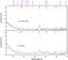 |
Fig. 1 The stacked RGS spectra (in the observed frame) in 2013–2014 (upper panel) and 2016 (lower panel, rebinned for clarity). |
Photoionized models of the emission features for NGC 5548.
3.2.2 The 2016 RGS spectrum
In the global fit of the 2016 spectrum, the power-law component, the reflection component, the two XABS components (Sect. 3.2) are allowed to vary. Assuming the X-ray emitter remains unchanged between the two epochs (Sect. 3.1), with Model T for the narrow and broad emission features, the best-fit C-stat over expected C-stat ratio is 1443/1304 for the RGS band. Contrary to our simple assumption that the narrow emission features are constant between thetwo epochs, we do find that the forbidden lines of O VII and N vi are underestimated in our model when applied to the 2016 spectrum. These results are similar to what we found with the simple phenomenological fit (Sect. 3.1). Figure 6 shows the comparison of the best-fit model to both spectra in 2013–2014 and 2016.
4 Discussion
4.1 In relation to the optical NELR
From the variability of the optical narrow emission line [O iii] 4959 Å and 5007 Å, Peterson et al. (2013) deduced that the optical narrow emission line region (NELR) has a radius of 1–3 pc with ne ~ 1011 m−3. A variability study of the X-ray narrow emission line [O VII] 22.10 Å yields an X-ray NELR distance of 1–15 pc (Detmers et al. 2009), which is consistent with the optical NELR. We cannot constrain the density and distance in the X-ray spectra. Although the He-like triplet of O VII is prominent, the associated density diagnostic is not effective, since the forbidden to intercombination line ratio of O VII is strongly sensitive to the density only when ne ~ 1015−18 m−3 (Porquet & Dubau 2000, their Fig. 10), which is too high for the NELR.
The asymmetric line profiles of the [O iii] lines indicate that the NELR has an outflowing component, with HWHM_blue∕HWHM_red ≃ 2.12 with an outflow velocity of ~460 km s−1 (Peterson et al. 2013). Similarly, the line profile of O VII observed in the X-ray band is also asymmetric (see Fig. 3 in Whewell et al. 2015). This can also be seen in our Models D and T, where two emission components with different outflow velocities are required. The emission component (EM 2) that dominates the forbidden lines of O VII and N vi (but not that of Ne ix, see Fig. 4) is blueshifted (~ −400 km s−1). The other emission component (EM 1), which dominates the Lyα lines of O VIII, N VII and C vi (Fig. 4), has a negligible outflow velocity. Such divergent kinematic behaviour can also be found in the phenomenological fit by Whewell et al. (2015, their Table 6).
We point out that Peterson et al. (2013) attribute the velocity broadening to the virial motion of the gas and no microscopic turbulence velocity broadening is taken into account. As pointed out by Kraemer et al. (2007), it is possible that microturbulence is present in the optical NELR of NGC 5548. Furthermore, if turbulence dissipates within the NELR, the plasma can be heated in excess of the temperature corresponding to photoionization. In our photoionization modeling of the X-ray narrow emission features, nondissipative microturbulence is taken into account. That is to say, the microscopic and macroscopic velocity broadening are both taken into account, but no extra heating is used to solve the thermal equilibrium.
In reality, it is possible that turbulence dissipates within the NELR, in practice, it is difficult to model the emergent spectrum. On one hand, the extra heating can be included via the external heating option in the PION model,3 if we know the scale length over which the turbulence dissipates, the plasma mass density and turbulence velocity of the photoionized plasma (Bottorff & Ferland 2002, their Eq. (1)). The dissipation scale length and direction, as well as the mass density, can only be assumed in our analysis. On the other hand, the line broadening might appear to be different for the resonance and forbidden lines. Considering a slab with suitable ionization parameter for the resonance and forbidden lines, assuming the turbulence dissipation direction is along the line of sight from the central engine toward the observer, and the dissipation length scale equals the size of the slab, the observed broadening of the forbidden lines is the integrated result of velocity broadening across the entire slab because they are optically thin. In contrast, due to the large optical depth, the observed resonance lines are only those escaping from the skin (τ ~ 1) of the far (with respect to the central engine) side of the slab, therefore, they are less broadened since turbulence converts to heating at the far side. In short, in order to model the emergent spectrum of a dissipative turbulent photoionized plasma, several assumptions are required, and the line broadening effect for resonance and forbidden lines are not trivial.
The bottom line is that the total velocity broadening of the narrow emission lines is 300–500 km s−1 for individual emission components, well in excess of the thermal broadening. Both the microscopic turbulence and macroscopic motions can contribute to the total velocity broadening, but the two velocities are highly degenerate (Fig. 5).
Furthermore, regardless of the number of emission components we used for the X-ray narrow emission features, the best-fit emission covering factor Ccov = Ω∕4π is rather small, with ~6% for Model S2, and 2–3% for the other models. This implies a compact geometry for the X-ray NELR. We caution that the photoionized plasma is assumed to be uniform with the PION model. If the NELR is clumpy, then the true covering factor can be larger. On the other hand, the optical NELR of NGC 5548 is also found to be compact (Ccov ~ 11%, Kraemer et al. 1998).
To summarize, in this work, the X-ray narrow emission features show asymmetric line profiles, and the underlying photoionized plasma is turbulent and compact in size. Similar results have been reported in previous optical studies of the NELR (Kraemer et al. 1998, 2007; Peterson et al. 2013). Moreover, distance estimates (from previous studies) of the X-ray and optical NELR indicate that the two regions might be co-located, i.e. a few parsec away from the central engine (Detmers et al. 2009; Peterson et al. 2013; Landt et al. 2015). These similarities further suggest that the X-ray and optical NELR might be the same multi-phase photoionized plasma that manifests its emission in different energy bands. This interpretation has actually been established with the radiation pressure confinement (RPC) model (e.g. Stern et al. 2014). Of course, the RPC model is more sophisticated, where the multi-phase photoionized plasma has a range of number densities and ionization parameters. We only have two uniform slabs for the X-ray narrow emission features. But we do notice that the radiation to gas pressure ratio decreases from the highly ionized component EM 1 to the lowly ionized component EM 2 (Sect. 3.2.1), which agrees with the RPC model.
Interestingly, based on the measurement of the metastable absorption lines (C iii 1175 Å and Si iii 1298 Å) in the UV band, Arav et al. (2015) determined the number density (log ne = 10.8 ± 0.1 m−3) and distance (~3.5 pc) of the UV absorption component 1, which are also similar to those of the optical NELR.
4.2 In relation to the X-ray warm absorber
As can be seen from Table 3, the single-phase emission component fully covered by the warm absorber components A+B+C (Whewell et al. 2015, i.e. Model S2 in this work) and the two-phase emission components with no overlying warm absorber components (Model D) yield comparable fit statistics. Nevertheless, the underlying geometries of the two scenarios are rather different.
In the first scenario (Model S2), the warm absorber components (A to C) are located between the X-ray emitter and the observer, with the warm absorber components fully covering the emission component. Given that the X-ray NELR is compact in size (Sect. 4.1), full covering by the warm absorber components is possible, as long as the warm absorber components are located further away than the emission component. Ebrero et al. (2016) estimate the distances of the warm absorber components via a variability study. The warm absorber components A and B are at least 10 pc away from the central engine, while component C is between 1 and 5 pc (Fig. 7).
Nevertheless, a distance estimation based on the density sensitive metastable absorption lines found a 3σ upper limit of 0.23 pc for the warm absorber component B (Mao et al. 2017). If this is the case, and assuming the X-ray NELR has a distance of 1–3 pc, the warm absorber component B cannot absorb the NELR. The second scenario (Model D), with no overlying absorption, does not suffer from the logical difficulty, if the warm absorber component B is closer than the X-ray NELR.
Distance (and also density) estimation using either timing or spectral analysis is challenging. Timing analyses usually suffer from low cadence and sometimes the signal-to-noise ratio is not enough to claim a significant change. On the other hand, spectral analyses (in the X-ray band) suffer from low spectral resolution and limited photon collecting area in the relevant energy band with current grating spectrometers. Future studies with either an intensive monitoring program or a spectral analysis with the next generation spectrometers (e.g. Arcus, Smith et al. 2016)are required to better constrain the number density and distance of the warm absorber (Kaastra et al. 2017).
We also compare the parameters of the emission and absorption components. We list the parameters for selected emission and absorption comparison in Table 4. The term nH r2 of the X-ray emission component 1, (X-ray) warm absorber component B and UV absorption component 1 are comparable (~ 1044 m−1). The distances (thus number densities) of EM 1 is consistent with UV 1, but not with X-ray component B (Fig. 7). The other parameters (NH, vout, and vmic) of these emission and absorption components do not agree with each other. For the X-ray absorption component A and X-ray emission component 2, three parameters (nHr2, ovout and vmic) are roughly of the same order of magnitude, but the hydrogen column density and distance (thus number density) are not consistent with each other.
The warm absorber components C to E have similar distances as the X-ray NELR (Fig. 7), but the inferred number densities are lower by an order of magnitude, while component F has smaller distance and number density than the X-ray NELR (Ebrero et al. 2016). The UV absorption components 3 and 5 are slightly further away (5–15 pc) than the X-ray NELR, while the distances of components 2, 4, and 6 are not well constrained (Arav et al. 2015).
In short, the emission components are not the counterpart of the UV/X-ray absorption components outside the line of sight.
Comparing the parameters of selected emission and absorption components.
4.3 Unobscured SED for the X-ray emitter
Although we have witnessed significant spectral changes since June 20114 (Kaastra et al. 2014), we argue that using the unobscured SED for the X-ray emitter (same in Whewell et al. 2015) is reasonable given the following effects.
First, there is a geometric effect. A possible geometry is shown in Fig. 4 of Kaastra et al. (2014), where the obscurer appears along our line of sight, yet only a small part is in-between the narrow line region and the black hole and the accretion disk.
Second,there is a time delay effect. It is also possible that the X-ray emitter has not yet responded to the changes in the ionizing SED, whether it is obscured or not. The delay timescale (τdelay) is the sum of the light travel time (τlt) and the recombination time (τrec). The recombination timescale mainly depends on the number density (nH ) of the plasma (Krolik & Kriss 1995; Nicastro et al. 1999). The higher the plasma density, the shorter the recombination time. In our photoionization modeling, the recombination timescale for O VII is roughly on the order of  . The light travel time is simply 3.26 (rX∕pc) yr, i.e., 108 (rX∕pc) s, where rX is the distance of the X-ray NELR. As long as the number density of the photoionized plasma is ≳ 1010 m−3 and the distance of the X-ray NELR ≳1 pc, the delay time (≳3.3 yr) is longer than the time separation (~2.6 yr) between ourtwo epochs (2013–2014 and 2016).
Third, there is a low-density effect. When the density of the photoionized plasma is sufficiently low, the recombination timescale (τrec) is orders of magnitude higher than the variability timescale (τvar), and the plasma is in a quasi-steady state. In other words, the ionization balance of the plasma varies slightly around the mean value corresponding to the mean ionizing flux level over time (Nicastro et al. 1999; Kaastra et al. 2012; Silva et al. 2016).
4.4 A charge exchange component?
In our physical global fit (Sect. 3.2) to the stacked RGS spectrum in 2013–2014, we find that the N VII Lyγ5 narrow emission line is abnormally high for a photoionized plasma (all panels in Fig. 3). When we include a Gaussian profile for the N VII Lyγ narrow emission line, the C-stat is significantly improved with ΔC = −23, at the price of two degrees of freedom. The best-fit line luminosity is (1.9 ± 0.5) × 1032 W, and the N VII Lyγ/Lyα ratio is  . Such a high Lyγ/Lyα ratio cannot be explained by a photoionized plasma, nor a collisionally ionized plasma, but it can be obtained with a charge exchange plasma (e.g. Gu et al. 2015).
It is possible for charge exchange events to occur if a warm (T ~ 105−6 K) outflow runs into the cold (T ≲ 1800 K) torus region. Assuming a constant radial velocity of ~300 km s−1, if the outflow is short-lived (≲102−3 yr), only gas arising beyond (Blustin et al. 2005) the broad line region can reach the torus region. If the outflow is long-lived, then outflows arising from the accretion disk (Proga 2000) can also reach the torus region. In fact, putative charge exchange emission features at 1223.6 Å, 1242.4 Å, and 1244.0 Å (for Ne x and S xv) in the UV spectrum of NGC 1275 have been reported in Gu et al. (2017).
In our case, using a charge exchange component (the CX model in SPEX, Gu et al. 2016), we can reproduce a N VII Lyγ/Lyα ratio of ~0.7, but the same CX plasma would also produce high Lyγ/Lyα for C vi and Lyδ/Lyα for O VIII ratios (~0.5), which are not found in the observed spectra. Therefore, we are not convinced that the N VII Lyγ/Lyα ratio alone can validate the presence of a charge exchange plasma in NGC 5548.
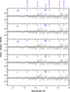 |
Fig. 2 The fit residuals of the physical models in the 7–18 Å band. |
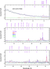 |
Fig. 4 The best-fit to the 2013–2014 RGS spectrum with three emission components (Model T) for the narrow and broad emission features. |
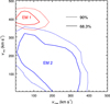 |
Fig. 5 The confidence level contours for the microscopic turbulence velocities (vmic) and macroscopic motion velocities (vmac) of EM 1 (in red) and 2 (in blue) in Model T. The solid and dotted contours refer to 68.3% (or Δ C = 2.30) and 90% (or Δ C = 4.61), respectively. |
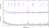 |
Fig. 6 With the model of three emission components (Model T), the best-fit to the RGS spectra (in the observed frame) in 2013–2014 (upper panel) and 2016 (lower panel, rebinned for clarity). |
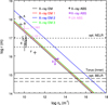 |
Fig. 7 Distance and number density of optical, UV and X-ray emission and/or absorption components in NGC 5548. The solid diagonal lines are the distance and density relations (i.e. log ξ =L∕nHr2) of the X-ray emission components (EM for Whewell et al. 2015, and EM 1–3 for Model T). The black pluses (1σ uncertainties) refer to the six warm absorber components (via a timing analysis, Ebrero et al. 2016). The purple arrows are the 3σ upper (distance) and lower (density) limits of the warm absorber component B (via a spectral analysis, Mao et al. 2017). The pink pluses are for the UV absorption components (Arav et al. 2015). The horizontal short dashed lines refer to the optical narrow emission line region (Peterson et al. 2013). The horizontal long dashed lines refer to the optical broad emission line region (Kaspi et al. 2000; Bottorff et al. 2002). The horizontal dotted line indicates the inner edge of the torus (Suganuma et al. 2006). |
5 Summary
We reanalyze the high-resolution spectrum of the archetypal Seyfert 1 galaxy NGC 5548 obtained with the Reflection Grating Spectrometer aboard XMM-Newton in 2013–2014 (770 ks), and analyze the spectrum in 2016 (70 ks). The main results are summarized as follows.
-
1.
The most prominent emission lines (the O VII forbidden line and O VIII Lyα line) are consistent (at a 1σ confidence level) between 2013–2014 and 2016. This is not totally unexpected, as the non-variability at such a timescale has beenreported previously.
-
2.
The X-ray narrow emission line region (NELR) can be modeled as a two-phase photoionized plasma without further absorption by the warm absorber. This is an alternative to the previous interpretation of the NELR as a single-phase photoionized plasma absorbed by some of the warm absorber components.
-
3.
The X-ray broad emission features can be modeled by a third photoionized component.
-
4.
Our X-ray spectral analysis found that the line profiles of the narrow emission lines are asymmetric, the photoionized plasma is turbulent and the emission region is compact in size. Similar results have been found in the optical studies. Furthermore, distance estimates, from literature, of the X-ray and optical narrow emission line regions suggest that they might be co-located. Therefore, it is possible that the multi-phase nature of the NELR manifests its emission in different energy bands.
-
5.
Future missions like Arcus are in need in order to better constraints on the distances of the warm absorber components. Hence, we can tell whether the warm absorber intervenes along the line of sight from the X-ray narrow line emitter to the observer.
-
6.
The X-ray NELR is not the counterpart of the UV/X-ray absorber outside the line of sight.
-
7.
The N VII Lyγ to Lyα ratio is abnormally high in the stacked RGS spectra in 2013–2014. We investigate the possibility that this line may be produced by charge exchange.
Acknowledgements
This work is based on observations obtained with XMM-Newton, an ESA science mission with instruments and contributions directly funded by ESA Member States and the USA (NASA). SRON is supported financially by NWO, the Netherlands Organization for Scientific Research. The research at the Technion is supported by the I-CORE program of the Planning and Budgeting Committee (grant number 1937/12). JM acknowledges discussions with M. Whewell. EC is partially supported by the NWO-Vidi grant number 633.042.525. SB acknowledges financial support from the Italian Space Agency under grant ASIINAFI/037/12/0, and from the European Union Seventh Framework Programme (FP7/2007-2013) under grant agreement no. 31278. LDG acknowledges support from the Swiss National Science Foundation. POP acknowledges financial support from the French CNES. GP acknowledges support from the Bundesministerium für Wirtschaft und Technologie/Deutsches Zentrum für Luft- und Raumfahrt (BMWI/DLR, FKZ 50 OR 1604) and the Max Planck Society. EB is grateful for funding from the European Union’s Horizon 2020 research and innovation programme under the Marie Sklodowska-Curie grant agreement no. 655324.
References
- Arav, N., Chamberlain, C., Kriss, G. A., et al. 2015, A&A, 577, A37 [NASA ADS] [CrossRef] [EDP Sciences] [Google Scholar]
- Armentrout, B. K., Kraemer, S. B., & Turner, T. J. 2007, ApJ, 665, 237 [NASA ADS] [CrossRef] [Google Scholar]
- Arnaud, K. A. 1996, Astron. Data Anal. Softw. Syst. V, 101, 17 [Google Scholar]
- Bautista, M. A., & Kallman, T. R. 2001, ApJS, 134, 139 [NASA ADS] [CrossRef] [Google Scholar]
- Bennert, N., Jungwiert, B., Komossa, S., Haas, M., & Chini, R. 2006a, A&A, 459, 55 [NASA ADS] [CrossRef] [EDP Sciences] [Google Scholar]
- Bennert, N., Jungwiert, B., Komossa, S., Haas, M., & Chini, R. 2006b, A&A, 456, 953 [NASA ADS] [CrossRef] [EDP Sciences] [Google Scholar]
- Bhardwaj, A. 2006, Adv. Geosci., 3, 215 [Google Scholar]
- Bianchi, S., Guainazzi, M., & Chiaberge, M. 2006, A&A, 448, 499 [NASA ADS] [CrossRef] [EDP Sciences] [Google Scholar]
- Bianchi, S., Chiaberge, M., Evans, D. A., et al. 2010, MNRAS, 405, 553 [NASA ADS] [Google Scholar]
- Blustin, A. J., Page, M. J., Fuerst, S. V., Branduardi-Raymont, G., & Ashton, C. E. 2005, A&A, 431, 111 [NASA ADS] [CrossRef] [EDP Sciences] [Google Scholar]
- Bottorff, M., & Ferland, G. 2002, ApJ, 568, 581 [NASA ADS] [CrossRef] [Google Scholar]
- Bottorff, M. C., Baldwin, J. A., Ferland, G. J., Ferguson, J. W., & Korista, K. T. 2002, ApJ, 581, 932 [NASA ADS] [CrossRef] [Google Scholar]
- Cappi, M., De Marco, B., Ponti, G., et al. 2016, A&A, 592, A27 [NASA ADS] [CrossRef] [EDP Sciences] [Google Scholar]
- Chiang, J., Reynolds, C. S., Blaes, O. M., et al. 2000, ApJ, 528, 292 [NASA ADS] [CrossRef] [Google Scholar]
- Costantini, E., Kaastra, J. S., Arav, N., et al. 2007, A&A, 461, 121 [NASA ADS] [CrossRef] [EDP Sciences] [Google Scholar]
- Costantini, E., Kriss, G., Kaastra, J. S., et al. 2016, A&A, 595, A106 [NASA ADS] [CrossRef] [EDP Sciences] [Google Scholar]
- de Plaa, J., Kaastra, J. S., Tamura, T., et al. 2004, A&A, 423, 49 [NASA ADS] [CrossRef] [EDP Sciences] [Google Scholar]
- de Vaucouleurs, G., de Vaucouleurs, A., Corwin, H. G., Jr., et al. 1991, Third Ref. Catalogue of Bright Galaxies. Version 3.9 [Google Scholar]
- den Herder, J. W., Brinkman, A. C., Kahn, S. M., et al. 2001, A&A, 365, L7 [NASA ADS] [CrossRef] [EDP Sciences] [Google Scholar]
- Dennerl, K. 2010, Space Sci. Rev., 157, 57 [NASA ADS] [CrossRef] [Google Scholar]
- Detmers, R. G., Kaastra, J. S., Costantini, E., McHardy, I. M., & Verbunt, F. 2008, A&A, 488, 67 [NASA ADS] [CrossRef] [EDP Sciences] [Google Scholar]
- Detmers, R. G., Kaastra, J. S., & McHardy, I. M. 2009, A&A, 504, 409 [NASA ADS] [CrossRef] [EDP Sciences] [Google Scholar]
- Di Gesu, L., Costantini, E., Ebrero, J., et al. 2015, A&A, 579, A42 [NASA ADS] [CrossRef] [EDP Sciences] [Google Scholar]
- Ebrero, J., Kaastra, J. S., Kriss, G. A., et al. 2016, A&A, 587, A129 [NASA ADS] [CrossRef] [EDP Sciences] [Google Scholar]
- Ferland, G. J., Chatzikos, M., Guzmán, F., et al. 2017, Rev. Mex. Astron. Astrofís., 53, 385 [Google Scholar]
- Gu, L., Kaastra, J., Raassen, A. J. J., et al. 2015, A&A, 584, L11 [NASA ADS] [CrossRef] [EDP Sciences] [Google Scholar]
- Gu, L., Kaastra, J., & Raassen, A. J. J. 2016, A&A, 588, A52 [NASA ADS] [CrossRef] [EDP Sciences] [Google Scholar]
- Gu, L., Mao, J., O’Dea, C. P., et al. 2017, A&A, 601, A45 [NASA ADS] [CrossRef] [EDP Sciences] [Google Scholar]
- Guainazzi, M., & Bianchi, S. 2007, MNRAS, 374, 1290 [NASA ADS] [CrossRef] [Google Scholar]
- Guainazzi, M., Risaliti, G., Nucita, A., et al. 2009, A&A, 505, 589 [NASA ADS] [CrossRef] [EDP Sciences] [Google Scholar]
- Jansen, F., Lumb, D., Altieri, B., et al. 2001, A&A, 365, L1 [NASA ADS] [CrossRef] [EDP Sciences] [Google Scholar]
- Kaastra, J. S. 2017, A&A, 605, A51 [NASA ADS] [CrossRef] [EDP Sciences] [Google Scholar]
- Kaastra, J. S., & Bleeker, J. A. M. 2016, A&A, 587, A151 [NASA ADS] [CrossRef] [EDP Sciences] [Google Scholar]
- Kaastra, J. S., Mewe, R., & Nieuwenhuijzen, H. 1996, in UV and X-ray Spectroscopy of Astrophysical and Laboratory Plasmas, eds. K. Yamashita, & T. Watanabe (Tokyo: Univ. Acad. Press), 411 [Google Scholar]
- Kaastra, J. S., Mewe, R., Liedahl, D. A., Komossa, S., & Brinkman, A. C. 2000, A&A, 354, L83 [NASA ADS] [Google Scholar]
- Kaastra, J. S., Steenbrugge, K. C., Raassen, A. J. J., et al. 2002, A&A, 386, 427 [NASA ADS] [CrossRef] [EDP Sciences] [Google Scholar]
- Kaastra, J. S., de Vries, C. P., Steenbrugge, K. C., et al. 2011, A&A, 534, A37 [NASA ADS] [CrossRef] [EDP Sciences] [Google Scholar]
- Kaastra, J. S., Detmers, R. G., Mehdipour, M., et al. 2012, A&A, 539, A117 [NASA ADS] [CrossRef] [EDP Sciences] [Google Scholar]
- Kaastra, J. S., Kriss, G. A., Cappi, M., et al. 2014, Science, 345, 64 [NASA ADS] [CrossRef] [Google Scholar]
- Kaastra, J. S., Gu, L., Mao, J., et al. 2017, J. Instrum., 12, C08008 [CrossRef] [Google Scholar]
- Kallman, T., & Bautista, M. 2001, ApJS, 133, 221 [NASA ADS] [CrossRef] [Google Scholar]
- Kallman, T., Evans, D. A., Marshall, H., et al. 2014, ApJ, 780, 121 [NASA ADS] [CrossRef] [Google Scholar]
- Kaspi, S., Smith, P. S., Netzer, H., et al. 2000, ApJ, 533, 631 [NASA ADS] [CrossRef] [Google Scholar]
- Katsuda, S., Tsunemi, H., Mori, K., et al. 2011, ApJ, 730, 24 [NASA ADS] [CrossRef] [Google Scholar]
- Kinkhabwala, A., Sako, M., Behar, E., et al. 2002, ApJ, 575, 732 [NASA ADS] [CrossRef] [Google Scholar]
- Korista, K. T., Alloin, D., Barr, P., et al. 1995, ApJS, 97, 285 [NASA ADS] [CrossRef] [Google Scholar]
- Kraemer, S. B., Crenshaw, D. M., Filippenko, A. V., & Peterson, B. M. 1998, ApJ, 499, 719 [NASA ADS] [CrossRef] [Google Scholar]
- Kraemer, S. B., Bottorff, M. C., & Crenshaw, D. M. 2007, ApJ, 668, 730 [NASA ADS] [CrossRef] [Google Scholar]
- Krolik, J. H., & Kriss, G. A. 1995, ApJ, 447, 512 [NASA ADS] [CrossRef] [Google Scholar]
- Krolik, J. H., McKee, C. F., & Tarter, C. B. 1981, ApJ, 249, 422 [NASA ADS] [CrossRef] [Google Scholar]
- Laha, S., Guainazzi, M., Chakravorty, S., Dewangan, G. C., & Kembhavi, A. K. 2016, MNRAS, 457, 3896 [NASA ADS] [CrossRef] [Google Scholar]
- Landt, H., Ward, M. J., Steenbrugge, K. C., & Ferland, G. J. 2015, MNRAS, 454, 3688 [NASA ADS] [CrossRef] [Google Scholar]
- Lodders, K., Palme, H., & Gail, H.-P. 2009, Landolt Börnstein, 44 [Google Scholar]
- Longinotti, A. L., Nucita, A., Santos-Lleo, M., & Guainazzi, M. 2008, A&A, 484, 311 [NASA ADS] [CrossRef] [EDP Sciences] [Google Scholar]
- Mao, J., Kaastra, J. S., Mehdipour, M., et al. 2017, A&A 607, A100 [NASA ADS] [CrossRef] [EDP Sciences] [Google Scholar]
- Marinucci, A., Bianchi, S., Matt, G., et al. 2011, A&A, 526, A36 [NASA ADS] [CrossRef] [EDP Sciences] [Google Scholar]
- Mehdipour, M., Kaastra, J. S., Kriss, G. A., et al. 2015, A&A, 575, A22 [NASA ADS] [CrossRef] [EDP Sciences] [Google Scholar]
- Mehdipour, M., Kaastra, J. S., Kriss, G. A., et al. 2016a, A&A, 588, A139 [NASA ADS] [CrossRef] [EDP Sciences] [Google Scholar]
- Mehdipour, M., Kaastra, J. S., & Kallman, T. 2016b, A&A, 596, A65 [NASA ADS] [CrossRef] [EDP Sciences] [Google Scholar]
- Mehdipour, M., Kaastra, J. S., Kriss, G. A., et al. 2017, A&A, 607, A28 [NASA ADS] [CrossRef] [EDP Sciences] [Google Scholar]
- Netzer, H. 2015, ARA&A, 53, 365 [NASA ADS] [CrossRef] [Google Scholar]
- Nicastro, F., Fiore, F., Perola, G. C., & Elvis, M. 1999, ApJ, 512, 184 [NASA ADS] [CrossRef] [Google Scholar]
- Nucita, A. A., Guainazzi, M., Longinotti, A. L., et al. 2010, A&A, 515, A47 [NASA ADS] [CrossRef] [EDP Sciences] [Google Scholar]
- Peterson, B. M., Berlind, P., Bertram, R., et al. 2002, ApJ, 581, 197 [NASA ADS] [CrossRef] [Google Scholar]
- Peterson, B. M., Ferrarese, L., Gilbert, K. M., et al. 2004, ApJ, 613, 682 [NASA ADS] [CrossRef] [Google Scholar]
- Peterson, B. M., Denney, K. D., De Rosa, G., et al. 2013, ApJ, 779, 109 [NASA ADS] [CrossRef] [Google Scholar]
- Proga, D. 2000, ApJ, 538, 684 [NASA ADS] [CrossRef] [Google Scholar]
- Porquet, D., & Dubau, J. 2000, A&AS, 143, 495 [NASA ADS] [CrossRef] [EDP Sciences] [Google Scholar]
- Silva, C. V., Uttley, P., & Costantini, E. 2016, A&A, 596, A79 [NASA ADS] [CrossRef] [EDP Sciences] [Google Scholar]
- Smith, R. K., Abraham, M. H., Allured, R., et al. 2016, Proc. SPIE, 9905, 99054M [Google Scholar]
- Steenbrugge, K. C., Kaastra, J. S., Crenshaw, D. M., et al. 2005, A&A, 434, 569 [NASA ADS] [CrossRef] [EDP Sciences] [Google Scholar]
- Stern, J., Laor, A., & Baskin, A. 2014, MNRAS, 438, 901 [NASA ADS] [CrossRef] [Google Scholar]
- Suganuma, M., Yoshii, Y., Kobayashi, Y., et al. 2006, ApJ, 639, 46 [NASA ADS] [CrossRef] [Google Scholar]
- Ursini, F., Boissay, R., Petrucci, P.-O., et al. 2015, A&A, 577, A38 [NASA ADS] [CrossRef] [EDP Sciences] [Google Scholar]
- Wakker, B. P., Lockman, F. J., & Brown, J. M. 2011, ApJ, 728, 159 [NASA ADS] [CrossRef] [Google Scholar]
- Whewell, M., Branduardi-Raymont, G., Kaastra, J. S., et al. 2015, A&A, 581, A7 [NASA ADS] [CrossRef] [EDP Sciences] [Google Scholar]
The radiation to gas pressure ratio, also known as the pressure form of the ionization parameter, Ξ = L∕(4πr2nHckT) = ξ∕(4πckT), where L is the 1–1000 Ryd ionizing luminosity, r the distance of the slab, nH the hydrogen number density, k the Boltzmann constant and T the electron temperature (Krolik et al. 1981).
In Kraemer et al. (2007), the dissipative heating is introduced via the additional heating terms in the Cloudy modeling.
All Tables
The intrinsic (unabsorbed) luminosity of the prominent narrow emission features for the 2013–2014 and 2016 RGS spectra of NGC 5548.
All Figures
|
Fig. 1 The stacked RGS spectra (in the observed frame) in 2013–2014 (upper panel) and 2016 (lower panel, rebinned for clarity). |
| In the text | |
|
Fig. 2 The fit residuals of the physical models in the 7–18 Å band. |
| In the text | |
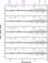 |
Fig. 3 As Fig. 2 in the 18–35 Å band. |
| In the text | |
|
Fig. 4 The best-fit to the 2013–2014 RGS spectrum with three emission components (Model T) for the narrow and broad emission features. |
| In the text | |
|
Fig. 5 The confidence level contours for the microscopic turbulence velocities (vmic) and macroscopic motion velocities (vmac) of EM 1 (in red) and 2 (in blue) in Model T. The solid and dotted contours refer to 68.3% (or Δ C = 2.30) and 90% (or Δ C = 4.61), respectively. |
| In the text | |
|
Fig. 6 With the model of three emission components (Model T), the best-fit to the RGS spectra (in the observed frame) in 2013–2014 (upper panel) and 2016 (lower panel, rebinned for clarity). |
| In the text | |
|
Fig. 7 Distance and number density of optical, UV and X-ray emission and/or absorption components in NGC 5548. The solid diagonal lines are the distance and density relations (i.e. log ξ =L∕nHr2) of the X-ray emission components (EM for Whewell et al. 2015, and EM 1–3 for Model T). The black pluses (1σ uncertainties) refer to the six warm absorber components (via a timing analysis, Ebrero et al. 2016). The purple arrows are the 3σ upper (distance) and lower (density) limits of the warm absorber component B (via a spectral analysis, Mao et al. 2017). The pink pluses are for the UV absorption components (Arav et al. 2015). The horizontal short dashed lines refer to the optical narrow emission line region (Peterson et al. 2013). The horizontal long dashed lines refer to the optical broad emission line region (Kaspi et al. 2000; Bottorff et al. 2002). The horizontal dotted line indicates the inner edge of the torus (Suganuma et al. 2006). |
| In the text | |
Current usage metrics show cumulative count of Article Views (full-text article views including HTML views, PDF and ePub downloads, according to the available data) and Abstracts Views on Vision4Press platform.
Data correspond to usage on the plateform after 2015. The current usage metrics is available 48-96 hours after online publication and is updated daily on week days.
Initial download of the metrics may take a while.