| Issue |
A&A
Volume 612, April 2018
|
|
|---|---|---|
| Article Number | A97 | |
| Number of page(s) | 16 | |
| Section | Astrophysical processes | |
| DOI | https://doi.org/10.1051/0004-6361/201732066 | |
| Published online | 04 May 2018 | |
Large-scale dynamos in rapidly rotating plane layer convection
1
School of Mathematics, Statistics and Physics, Newcastle University,
Newcastle upon Tyne,
NE1 7RU, UK
e-mail: This email address is being protected from spambots. You need JavaScript enabled to view it.
2
Leibniz-Institut für Astrophysik Potsdam,
An der Sternwarte 16,
11482
Potsdam, Germany
3
ReSoLVE Centre of Excellence, Department of Computer Science, Aalto University,
PO Box 15400,
00076
Aalto, Finland
4
Max-Planck-Institut für Sonnensystemforschung,
Justus-von-Liebig-Weg 3,
37077
Göttingen, Germany
5
Nordita, KTH Royal Institute of Technology and Stockholm University,
Roslagstullsbacken 23,
10691
Stockholm, Sweden
6
Department of Physics and Astronomy, Aichi University of Education, Kariya,
Aichi
446-8501, Japan
7
JILA and Department of Astrophysical and Planetary Sciences, University of Colorado,
Box 440,
Boulder,
CO 80303, USA
8
Department of Astronomy, AlbaNova University Center, Stockholm University,
10691
Stockholm, Sweden
9
Laboratory for Atmospheric and Space Physics,
3665 Discovery Drive,
Boulder,
CO 80303, USA
10
Aix Marseille Univ., CNRS, Centrale Marseille,
IRPHE UMR 7342,
Marseille, France
Received:
9
October
2017
Accepted:
15
January
2018
Abstract
Context. Convectively driven flows play a crucial role in the dynamo processes that are responsible for producing magnetic activity in stars and planets. It is still not fully understood why many astrophysical magnetic fields have a significant large-scale component.
Aims. Our aim is to investigate the dynamo properties of compressible convection in a rapidly rotating Cartesian domain, focusing upon a parameter regime in which the underlying hydrodynamic flow is known to be unstable to a large-scale vortex instability.
Methods. The governing equations of three-dimensional non-linear magnetohydrodynamics (MHD) are solved numerically. Different numerical schemes are compared and we propose a possible benchmark case for other similar codes.
Results. In keeping with previous related studies, we find that convection in this parameter regime can drive a large-scale dynamo. The components of the mean horizontal magnetic field oscillate, leading to a continuous overall rotation of the mean field. Whilst the large-scale vortex instability dominates the early evolution of the system, the large-scale vortex is suppressed by the magnetic field and makes a negligible contribution to the mean electromotive force that is responsible for driving the large-scale dynamo. The cycle period of the dynamo is comparable to the ohmic decay time, with longer cycles for dynamos in convective systems that are closer to onset. In these particular simulations, large-scale dynamo action is found only when vertical magnetic field boundary conditions are adopted at the upper and lower boundaries. Strongly modulated large-scale dynamos are found at higher Rayleigh numbers, with periods of reduced activity (grand minima-like events) occurring during transient phases in which the large-scale vortex temporarily re-establishes itself, before being suppressed again by the magnetic field.
Key words: convection / dynamo / instabilities / magnetic fields / magnetohydrodynamics (MHD) / methods: numerical
© ESO 2018
1 Introduction
In a hydromagnetic dynamo the motions in an electrically conducting fluid continuously sustain a magnetic field against the action of ohmic dissipation. Most astrophysical magnetic fields, including those in stars and planets, are dynamo-generated. In numerical simulations, turbulent motions almost invariably produce an intermittent magnetic field distribution that is correlated on the scale of the flow. However, most astrophysical objects exhibit magnetism that is organised on much larger scales. These large-scale fields might be steady or they may exhibit some time dependence. In the case of the Sun, for example, observations of surface magnetism (e.g. Stix 2002) indicate the presence of a large-scale oscillatory magnetic field in the solar interior that changes sign approximately every 11 years. Depending upon their age and spectral type, similar magnetic activity cycles can also be observed in other stars (e.g. Brandenburg et al. 1998). Whilst appearing to be comparatively steady on these timescales, the Earth’s predominantly dipolar field does exhibit long-term variations, occasionally even reversing its magnetic polarity (although rather irregular, a typical time span between reversals is of the order of 3 × 10⁵ years; see e.g. Jones 2011). Our understanding of the physical processes that are responsible for the production of large-scale magnetic fields in astrophysical objects relies heavily on mean-field dynamo theory (e.g. Moffatt 1978). This approach, in which the small-scale physics is parameterised in a plausible way, has had considerable success. However, despite much recent progress in this area, there are apparently contradictory findings, indicating that we still do not completely understand why large-scale magnetic fields appear to be so ubiquitous in astrophysics.
Convectively driven flows are a feature of stellar and planetary interiors where the effects of rotation can often play an important dynamical role via the Coriolis force. In the rapidly rotating limit, convective motions tend to be helical, leading to the expectation of a strong α-effect (an important regenerative term for large-scale magnetic fields in mean-field dynamo theory, usually a parameterised effect in simplified mean-field models). Many theoretical studies have therefore been motivated by the question of whether rotationally influenced convective flows can drive a large-scale dynamo in a fully self-consistent (i.e. non-parameterised) manner.
Using the Boussinesq approximation, in which the electrically conducting fluid is assumed to be incompressible, Childress & Soward (1972) were the first to demonstrate that a rapidly rotating plane layer of weakly convecting fluid was capable of sustaining a large-scale dynamo (see also Soward 1974). To be clear about terminology (here, and in what follows), we describe a plane layer dynamo as “large-scale” if it produces a magnetic field with a significant horizontally averaged component (such a magnetic field can also be described as “system-scale”; see e.g. Tobias et al. 2011). Building on the work of Childress & Soward (1972) and Soward (1974), many subsequent studies have explored the dynamo properties of related Cartesian Boussinesq models (Fautrelle & Childress 1982; Meneguzzi & Pouquet 1989; St. Pierre 1993; Jones & Roberts 2000; Rotvig & Jones 2002; Stellmach & Hansen 2004; Cattaneo & Hughes 2006; Favier & Proctor 2013; Calkins et al. 2015)and of the corresponding weakly stratified system (Mizerski & Tobias 2013). However, whilst near-onset rapidly rotating convection does produce a large-scale dynamo (see e.g. Stellmach & Hansen 2004), only small-scale dynamo action is observed in the rapidly rotating turbulent regime (Cattaneo & Hughes 2006), contrary to the predictions of mean-field dynamo theory. Indeed, Tilgner (2014) was able to identify an approximate parametric threshold (based on the Ekman number and the magnetic Reynolds number) above which small-scale dynamo action is preferred: low levels ofturbulence and a rapid rotation rate are found to be essential for a large-scale convectively driven dynamo.
There have been many fewer studies of the corresponding fully compressible system, so parameter space has not yet been explored to the same extent in this case. Käpylä et al. (2009) were the first to demonstrate that it is possible to excite a large-scale dynamo in rapidly rotating compressible convection at modestly supercritical values of the Rayleigh number (the key parameter controlling the vigour of the convective motions). However, it again appears to be much more difficult to drive a large-scale dynamo further from convective onset, with small-scale dynamos typically being reported in this comparatively turbulent regime (Favier & Bushby 2013). This is in agreement with the Boussinesq studies, such as Cattaneo & Hughes (2006). Moreover, as noted by Guervilly et al. (2015), the transition from large-scale to small-scale dynamos in these compressible systems appears to occur in a similar region of parameter space to the Boussinesq transition that was identified by Tilgner (2014).
In rapidly rotating Cartesian domains, hydrodynamic convective flows just above onset are characterised by a small horizontal spatial scale (Chandrasekhar 1961). However, at slightly higher levels of convective driving, these small-scale motions can become unstable, leading to a large-scale vortical flow (Chan 2007). The width of these large-scale vortices is limited by the size of the computational domain; in these simulations, the corresponding flow field has a negligible horizontal average (unlike the large-scale magnetic fields described above). With increasing rotation rate, Chan (2007) observed a transition from cooler cyclonic vortices to warmer anticyclones, and subsequent fully compressible studies have found similar behaviour (Mantere et al. 2011; Käpylä et al. 2011; Chan & Mayr 2013). In corresponding Boussinesq calculations, Favier et al. (2014) and Guervilly et al. (2014) have found a clear preference for cyclonic vortices, and dominant anticyclones are never observed, although Stellmach et al. (2014) have found states consisting of cyclones and anticyclones (of comparable magnitude) at higher rotation rates. As noted by Stellmach et al. (2014) and Kunnen et al. (2016), this large-scale vortex instability is inhibited when no-slip boundary conditions are adopted at the upper and lower boundaries, so the formation of large-scale vortices depends to some extent upon the use of stress-free boundary conditions.
From the point of view of the convective dynamo problem, this large-scale vortex instability can play a very important role. In the rapidly rotating Boussinesq dynamo of Guervilly et al. (2015), the large-scale vortex leads directly to the production of magnetic fields at a horizontal wavenumber comparable to that of the large-scale vortex. Although the total magnetic energy in this case is less than 1% of the total kinetic energy, the resultant magnetic field is locally strong enough to inhibit the large-scale flow. This temporarily suppresses the dynamo until the magnetic field becomes weak enough for the vortical instability to grow again. In some sense, the dynamo in this case switches on and off as the energy in the large-scale flow fluctuates.
In the fully compressible regime, the large-scale vortex instability has been shown to produce a different type of dynamo (Käpylä et al. 2013; Masada & Sano 2014a,b). As in the Boussinesq case that was considered by Guervilly et al. (2015), the large-scale flow produces a large-scale magnetic field which exhibits some time dependence. However, whilst the large-scale vortex is again suppressed once the magnetic field becomes dynamically significant, these dynamos are able to persist without the subsequent regeneration of these vortices (suggesting that these dynamos may be a compressible analogue of the dynamo considered by Childress & Soward 1972, albeit operating in the strong field limit). Once established, the magnetic energy in these dynamos is comparable to the kinetic energy of the system, with the horizontal components of the large-scale magnetic field oscillating in a regular manner, with a phase shift of approximately π∕2 between the two components, leading to a net rotation of the mean horizontal magnetic field. Although each component of the mean magnetic field certainly oscillates, because the temporal variation in the mean field essentially takes the form of a global rotation of the field orientation, it should be kept in mind that in a suitably corotating frame the mean field would appear statistically stationary.
The large-scale dynamo that was found by Käpylä et al. (2013) and Masada & Sano (2014a,b) is arguably the simplest known example of a moderately supercritical convectively driven dynamo in a rapidly rotating Cartesian domain. However, to achieve this non-linear magnetohydrodynamical state, any numerical code must successfully reproduce the large-scale vortex instability of rapidly rotating hydrodynamic convection in order to amplify a weak seed magnetic field. In the non-linear regime of the dynamo, the resultant large-scale magnetic field must then be sustained at a level that is (approximately) in equipartition with the local convective motions. As a result, this dynamo is an excellent candidate for a benchmarking exercise. Corresponding benchmarks exist for convectively driven dynamos in spherical geometry, both for Boussinesq (Christensen et al. 2001; Marti et al. 2014) and for anelastic fluids (Jones et al. 2011). To the best of our knowledge, there is no similar benchmark for a fully compressible, turbulent, large-scale dynamo.
The main aim of this paper is to further investigate the properties of this large-scale dynamo, focusing particularly upon the effects of varying the rotation rate and the convective driving, and upon the size of the computational domain. Wewill establish the regions of parameter space in which this dynamo can be sustained, looking at the ways in which the dynamo amplitude and cycle period depend upon the key parameters of the system. Most significantly, we will show that it is possible to induce strong temporal modulation in large-scale dynamos of this type by increasing the level of convective driving at fixed rotation rate. Finally, we carry out a preliminary code comparison (confirming the accuracy and validity of one particular solution via three independent codes) to assess whether this system could form the basis of a non-linear Cartesian dynamo benchmark, possibly involving broader participation from the dynamo community. In the next section, we set out our model and describe the numerical codes. Our numerical results are discussed in Sect. 3. In the final section we present our conclusions. The strengths and weaknesses of the proposed benchmark solution are described in Appendix A.
2 Governing equations and numerical methods
2.1 Model setup
We consider a plane layer of electrically conducting, compressible fluid, which is assumed to occupy a Cartesian domain of dimensions 0 ≤ x ≤ λd, 0 ≤ y ≤ λd, and 0 ≤ z ≤ d, where λ is the aspect ratio. This layer of fluid is heated from below, and the whole domain rotates rigidly about the vertical axis with constant angular velocity Ω = Ω 0ez. We define μ to be the dynamical viscosity of the fluid, whilst K is the radiative heat conductivity, η is the magnetic diffusivity, μ0 is the vacuum permeability, whilst cP and cV are the specific heat capacities at constant pressure and volume, respectively (as usual, we define γ = cP∕cV). All of these parameters are assumed to be constant, as is the gravitational acceleration g = −gez (z increases upwards). The evolution of this system is then determined by the equations of compressible magnetohydrodynamics, which can be expressed in the form
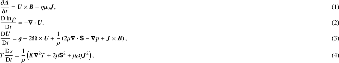 where A is the magnetic vector potential, U is the velocity, B = ∇×A is the magnetic field, J = ∇×B∕μ0 is the current density, ρ is the density, s is the specific entropy, T is the temperature, p is the pressure, and D∕Dt = ∂∕∂t + U ⋅∇ denotes the advective time derivative. The fluid obeys the ideal gas law with p = (γ − 1)ρe, where e = cVT is the internal energy. The traceless rate of strain tensor S is given by
 (5)
whilst the magnetic field satisfies
(5)
whilst the magnetic field satisfies
 (6)
(6)
Stress-free impenetrable boundary conditions are used for the velocity,
 (7)
and vertical field conditions for the magnetic field, i.e.
(7)
and vertical field conditions for the magnetic field, i.e.
 (8)
respectively (∇⋅B = 0 then impliesBz,z = 0 at z = 0, d). The temperature is fixed at the upper and lower boundaries. We adopt periodic boundary conditions for all variables in each of the two horizontal directions.
(8)
respectively (∇⋅B = 0 then impliesBz,z = 0 at z = 0, d). The temperature is fixed at the upper and lower boundaries. We adopt periodic boundary conditions for all variables in each of the two horizontal directions.
2.2 Non-dimensional quantities and parameters
Dimensionless quantities are obtained by setting
 (9)
where ρm is the initial density at z = zm = 0.5 d. The units of length, time, velocity, density, entropy, and magnetic field are
(9)
where ρm is the initial density at z = zm = 0.5 d. The units of length, time, velocity, density, entropy, and magnetic field are
![Mathematical equation: \begin{align*} & [x] = d,\;\; [t] = \sqrt{d/g},\;\; [U]=\sqrt{dg},\;\; [\rho]=\rho_{\textrm{m}},\\ \nonumber &[s]=c_{\textrm{P}},\;\; [B]=\sqrt{dg\rho _{\textrm{m}}\mu_0}. \end{align*}](/articles/aa/full_html/2018/04/aa32066-17/aa32066-17-eq7.png) (10)
(10)
Having non-dimensionalised these equations, the behaviour of the system is determined by various dimensionless parameters. Quantifying the two key diffusivity ratios, the fluid and magnetic Prandtl numbers are given by
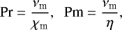 (11)
where νm = μ∕ρm is the mean kinematic viscosity and χm = K∕(ρmcP) is the mean thermal diffusivity. Defining HP to be the pressure scale height at zm, the mid-layer entropy gradient in the absence of motion is
(11)
where νm = μ∕ρm is the mean kinematic viscosity and χm = K∕(ρmcP) is the mean thermal diffusivity. Defining HP to be the pressure scale height at zm, the mid-layer entropy gradient in the absence of motion is
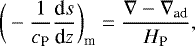 (12)
where ∇−∇ad is the superadiabatic temperature gradient with ∇ad = 1 − 1∕γ and
(12)
where ∇−∇ad is the superadiabatic temperature gradient with ∇ad = 1 − 1∕γ and  . The strength of the convective driving can then be characterised by the Rayleigh number,
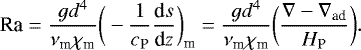 (13)
(13)
The amount of rotation is quantified by the Taylor number,
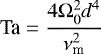 (14)
(which is related to the Ekman number, Ek, by Ek = Ta−1∕2). Since the critical Rayleigh number for the onset of hydrodynamic convection is proportional to Ta 2∕3 in the rapidly rotating regime (Chandrasekhar 1961), it is also useful to consider the quantity
(14)
(which is related to the Ekman number, Ek, by Ek = Ta−1∕2). Since the critical Rayleigh number for the onset of hydrodynamic convection is proportional to Ta 2∕3 in the rapidly rotating regime (Chandrasekhar 1961), it is also useful to consider the quantity
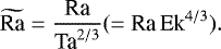 (15)
(see e.g. Julien et al. 2012). This rescaled Rayleigh number is a measure of the supercriticality of the convection that takes account of the stabilising influence of rotation. We also quote the convective Rossby number,
(15)
(see e.g. Julien et al. 2012). This rescaled Rayleigh number is a measure of the supercriticality of the convection that takes account of the stabilising influence of rotation. We also quote the convective Rossby number,
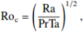 (16)
which is indicative of the strength of the thermal forcing compared to the effects of rotation.
(16)
which is indicative of the strength of the thermal forcing compared to the effects of rotation.
Whilst Ra, Ta, and Pr are input parameters that must be specified at the start of each simulation, it is possible to measure a number of useful quantities based on system outputs. These are expressed here in dimensional form for ease of reference. We define the fluid and magnetic Reynolds numbers via
 (17)
where kf = 2π∕d is indicative of the vertical scale of variation of the convective motions, and urms is the time-average of the rms velocity during the saturated phase of the dynamo. The time-evolution of the rms velocity, Urms(t), is also considered, but only its constant time-averaged value will be used to define other diagnostic quantities. The quantity urms kf is therefore an estimate of the inverse convective turnover time in the non-linear phase of the dynamo. The Coriolis number, an alternative measure of the importance of rotation (compared to inertial effects) is given by
(17)
where kf = 2π∕d is indicative of the vertical scale of variation of the convective motions, and urms is the time-average of the rms velocity during the saturated phase of the dynamo. The time-evolution of the rms velocity, Urms(t), is also considered, but only its constant time-averaged value will be used to define other diagnostic quantities. The quantity urms kf is therefore an estimate of the inverse convective turnover time in the non-linear phase of the dynamo. The Coriolis number, an alternative measure of the importance of rotation (compared to inertial effects) is given by
 (18)
(18)
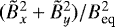
All of the simulations described in this paper have Co ≳ 4 (and Ro_c < 0.4) so are in a rotationally dominated regime1. Finally, the equipartition magnetic field strength is defined by
 (19)
where angle brackets denote volume averaging.
(19)
where angle brackets denote volume averaging.
2.3 Initial conditions
All of the simulations in this paper are initialised from a hydrostatic state corresponding to a polytropic layer, for which p ∝ ρ1+1∕m, where m is the polytropic index. Assuming a monatomic gas with γ = 5∕3, we adopt a polytropic index of m = 1 throughout. This gives a superadiabatic temperature gradient of ∇−∇ad = 1∕10, so the layer is convectively unstable, as required. The degree of stratification is determined by specifying a density contrast of 4 across the layer. To be as clear as possible about our proposed benchmark case (see Appendix A for details), it is useful to provide explicit functional forms for the initial density, pressure, and temperatureprofiles in our dimensionless units. Recalling that the layer has a unit depth and that ρm = 1, the initial density profile is given by
![Mathematical equation: \[ \rho(z) = \frac{2}{5}(4-3z), \]](/articles/aa/full_html/2018/04/aa32066-17/aa32066-17-eq18.png) whilst the initial pressure and temperature profiles are given by
whilst the initial pressure and temperature profiles are given by
![Mathematical equation: \[ p(z) = \frac{1}{15}(4-3z)^2, \]](/articles/aa/full_html/2018/04/aa32066-17/aa32066-17-eq19.png) and
and
![Mathematical equation: \[ T(z) = \frac{5}{12}(4-3z), \]](/articles/aa/full_html/2018/04/aa32066-17/aa32066-17-eq20.png) respectively. The fixed temperature boundary conditions imply that T (0) = 5∕3 and T (1) = 5∕12 (independent of x and y, for all time). These profiles are consistent with a dimensionless pressure scale height of HP = 1∕6 at the top of the domain, which is an alternative way of specifying the level of stratification. Since the governing equations are formulated in terms of the specific entropy, it is worth noting that these initial conditions are consistent with an initial entropy distribution of the form
respectively. The fixed temperature boundary conditions imply that T (0) = 5∕3 and T (1) = 5∕12 (independent of x and y, for all time). These profiles are consistent with a dimensionless pressure scale height of HP = 1∕6 at the top of the domain, which is an alternative way of specifying the level of stratification. Since the governing equations are formulated in terms of the specific entropy, it is worth noting that these initial conditions are consistent with an initial entropy distribution of the form
![Mathematical equation: \[ s = \ln \left(\frac{T(z)}{T_{\textrm{m}}}\right) - \frac{2}{5}\ln\left(\frac{p(z)}{p_{\textrm{m}}}\right), \]](/articles/aa/full_html/2018/04/aa32066-17/aa32066-17-eq21.png) where Tm = 25∕24 and pm = 5∕12 are the mid-layer values of the temperatureand pressure, respectively (sm = 0 with this normalisation).
where Tm = 25∕24 and pm = 5∕12 are the mid-layer values of the temperatureand pressure, respectively (sm = 0 with this normalisation).
In all simulations, convection is initialised by weakly perturbing this polytropic state in the presence of a low amplitude seed magnetic field (which varies over short length scales, with zero net flux across the domain). The precise details of these initial perturbations do not strongly influence the nature of the final non-linear dynamos, although it goes without saying that the early evolution of this system does depend upon the initial conditions that are employed (as illustrated in Appendix A).
2.4 Numerical methods
The PENCIL CODE2 (Code 1) is a tool for solving partial differential equations on massively parallel architectures. We use it in its default configuration in which the MHD equations are solved as stated in Eqs. (1)–(4). First and second spatial derivatives are computed using explicit centred sixth-order finite differences. Advective derivatives of the form U ⋅ ∇ are computed using a fifth-order upwinding scheme, which corresponds to adding a sixth-order hyperdiffusivity with the diffusion coefficient |U|δx5∕60 (Dobler et al. 2006). For the time stepping we use the low-storage Runge-Kutta scheme of Williamson (1980). Boundary conditions are applied by setting ghost zones outside the physical boundaries and computing all derivatives on and near the boundary in the same fashion. The non-dimensionalising scalings that have been described above correspond directly to those employed by Code 1. Whilst the other codes that have been used (see below) employ different scalings, we have rescaled results from these to ensure direct comparability with the results from the PENCIL CODE.
The second code that is used in this paper (Code 2) is an updated version of the code that was originally described by Matthews et al. (1995). The system of equations that is solved is entirely equivalent to that presented in Sect. 2.1, but instead of time-stepping evolution equations for the magnetic vector potential, the logarithm of the density, the velocity field, and the specific entropy, this code solves directly for the density, velocity field, and temperature (see e.g. Matthews et al. 1995), whilst a poloidal-toroidal decomposition is used for the magnetic field. Due to the periodicity in both horizontal directions, horizontal derivatives are computed in Fourier space using standard fast Fourier transform libraries. In the vertical direction, a fourth-order finite difference scheme is used, adopting an upwind stencil for the advective terms. The time-stepping is performed by an explicit third-order Adams-Bashforth technique, with a variable time-step. As noted above, this code adopts a different set of non-dimensionalising scalings to those described in Sect. 2.2 (see Favier & Bushby 2012, for more details).
Code 3 is based upon a second-order Godunov-type finite-difference scheme that employs an approximate MHD Riemann solver with operator splitting (Sano et al. 1999; Masada & Sano 2014a,b). The hydrodynamical part of the equations is solved by a Godunov method, using the exact solution of the simplified MHD Riemann problem. The Riemann problem is simplified by including only the tangential component of the magnetic field. The characteristic velocity is then that of the magneto-sonic wave alone, and the MHD Riemann problem can be solved in a way similar to the hydrodynamical one (Colella & Woodward 1984). The piecewise linear distributions of flow quantities are calculated with a monotonicity constraint following the method of van Leer (1979). The remaining terms, the magnetic tension component of the equation of motion and the induction equation, are solved by the Consistent MoC-CT method (Clarke 1996), guaranteeing ∇ ⋅ B = 0 to within round-off error throughout the calculation (Evans & Hawley 1988; Stone & Norman 1992).
3 Results
3.1 Reference solution
In this section, we present a detailed description of a typical dynamo run exhibiting large-scale dynamo action (carried out using Code 2). This case, which will henceforth be referred to as the reference solution, forms the basis for the proposed benchmark calculation that is discussed in Appendix A (with the corresponding calculations denoted by cases A1, A2, and A3 in the upper three rows of Table 1 where our parameter choices are also summarised). For numerical convenience, we fix Pr = Pm = 1 for the reference solution, whilst our choice of Ta = 5 × 10⁸ ensures that rotation plays a significant role in the ensuing dynamics. Defining Ra crit to be the critical Rayleigh number at which the hydrostatic polytropic state becomes linearly unstable to convective perturbations, it can be shown that Racrit = 6.006 × 10⁶ for this set of parameters. This critical value (here quoted to three decimal places) was determined using an independent Newton–Raphson–Kantorovich boundary value solver for the corresponding linearised system. At onset, the critical horizontal wavenumberfor the convective motions is very large (in these dimensionless units, the preferred horizontal wavenumber at onset is given by k ≈ 36), indicating apreference for narrow convective cells. Our choice of Rayleigh number, Ra = 2.4 × 10⁷ ≈ 4 Racrit, is moderately supercritical. However, we would still expect small-scale convective motions during the early phases of the simulation. Our choice of λ = 2 for the aspect ratio of the domain is small enough to enable us to properly resolve these motions, whilst also being large enough to allow the expected large-scale vortex instability to grow.
Summary of the simulations in this paper.
3.1.1 Large-scale dynamo
Figure 1 shows the time evolution of Urms(t) and Brms(t), the rms velocity and magnetic field, for the reference solution. Whilst the rms quantities have been left in dimensionless form, time has been normalised by the inverse convective turnover time during the final stages of the simulation, by which time the system is in a statistically steady state. Initially, there is a very brief period of exponential growth (spanning no more than a few convective turnover times), followed by a similarly rapid reduction in the magnitude of Urms(t). At these very early times, the convective motions are (as expected from linear theory) characterised by a small horizontal length scale. The solution then enters a prolonged phase of more gradual evolution, lasting until time turmskf ≈ 470, during which time Urms(t) tends to increase. This period of growth coincides with a gradual transfer of energy from small to large scales, leading eventually to a convective state that is dominated by larger scales of motion. This is an example of the large-scale vortex instability that was discussed in Sect. 1.
The transition from small to large-scale convection is clearly illustrated by the time evolution of the corresponding temperaturedistribution. The upper two plots in Fig. 2 show the mid-layer temperature distribution at time turmskf = 3.4, at which point the motions have a small horizontal length scale, and time turmskf = 362.0, at which the temperaturedistribution varies over the largest available scale. The lower plot shows the corresponding kinetic energy spectra as a function of the horizontal wavenumber, k, at times turmskf = 3.4 and turmskf = 362.0. As expected from linear theory, most of the power at time turmskf = 3.4 is concentrated at relatively high wavenumbers. Defining k1 = 2π∕λ (in this domain, k1 = π) to be the fundamental mode, corresponding to one full oscillation across the width of the domain, the corresponding kinetic energy spectrum peaks at around k∕k1 = 9 at this early time. This implies a favoured horizontal wavenumber of k ≈ 28.3 in these dimensionless units. This is comparable to the critical wavenumber at convective onset. At time turmskf = 362.0 there is still significant energy in the higher wavenumber, small-scale components of the flow (the spectrum is now broader, extending to higher wavenumbers than before). However, most of the power in the kinetic energy spectrum has been transferred to the k∕k1 = 1 component. This corresponds to the large-scale vortex. Even at turmskf = 3.4 there are some indications of non-monotonicity in the power spectrum at low wavenumbers, so this instability sets in very rapidly as the system evolves.
As Urms(t) (or, equivalently, the kinetic energy in the system) increases, it soon reaches a level above which the flow is sufficiently vigorous to excite a dynamo. The seed magnetic field is initially very weak, with Brms(t) many orders of magnitude smaller than the typical values of Urms(t). However, asillustrated in Fig. 1, once the large-scale vortex instability starts to grow, Brms(t) also starts to increase. With increasing Urms(t) (effectively, an ever-increasing magnetic Reynolds number during this growth phase), the growth of Brms(t) accelerates until it reaches a point at which the magnetic field is strong enough to exert a dynamical influence upon the flow. The sharp decrease in Urms(t) at time turmskf ≈ 470 is an indicator of the effects of the Lorentz force upon the flow, with the large-scale mode being strongly suppressed by the magnetic field. After this point, which marks the start of the non-linear phase of the dynamo, a more gradual growth of Brms(t) is accompanied by a gradual decrease in Urms(t). By the time turmskf ≈ 1600, the dynamo appears to reach a statistically steady state in which Brms(t) is comparable to Urms(t), which itself is comparable to the rms velocity before the large-scale vortex started to develop. The ohmic decay time, τη (based on the depth of the layer), corresponds to ≈2300 convective turnover times. So having continued this calculation to turmskf ≈ 4250, observing no significant changes in Brms or urms over the latter half of the simulation, we can be very confident that this is a persistent dynamo solution that will not decay over longer times.
Having discussed the time evolution of the system, we now turn our attention to the form of the magnetic field. Figure 3 shows the time- and z-dependence of the horizontally averaged profiles for Bx and By, as well as the kinetic and magnetic energy spectra at the end of the dynamo run. Here the  (for i = x or y) represent horizontally averaged magnetic field components, whilst the
  correspond to volume averages. It is clear from these plots that the magnetic field distribution has no significant mean horizontal component (compared to its equipartition value) when the dynamo enters the non-linear phase (at turmskf ≈ 470). However, as the dynamo evolves from turmskf ≈ 470, a cyclically varying mean horizontal field gradually emerges, eventually growing to a level at which the peak mean horizontal field almost reaches the equipartition level (although it should be noted that the peak amplitude does vary somewhat, from one cycle to the next). This mean magnetic field is approximately symmetric about the mid-plane with no real indication of any propagation of activity either towards or away from this mid-plane. The cycle period, τcyc, is approximately 1000 convective turnover times, which is of a similar order of magnitude to the ohmic decay time quoted above (τcyc ≈ 0.5τη). The dominance of the large-scale magnetic field is confirmed by the presence of a pronounced peak at k∕k1 = 0 in the magnetic energy spectrum that is shown in the lower part of Fig. 3. It should be stressed again that the kinetic energy spectrum is peaked at small scales at this stage, so the large-scale vortex (which plays a critical role in initialising the dynamo) no longer appears to have a significant role to play in this large-scale dynamo. This is emphasised by the lack of a significant k∕k1 = 1 peak in the kinetic energy spectrum.
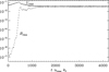 |
Fig. 1 Time evolution of Urms(t) and Brms(t) for the reference solution. Time has been normalised by the inverse convective turnover time in the final non-linear state. |
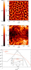 |
Fig. 2 Early stages of the reference solution. Mid-layer temperature distributions (at zm) at times turmskf = 3.4 (top) and turmskf = 362.0 (middle), plotted as functions of x and y. In each plot, the mid-layer temperature is normalised by its mean value (horizontally averaged), with the contours showing the deviations from the mean. Bottom: mid-layer kinetic energy spectra at the same times, normalised by the average kinetic energy at zm at each time. Here k is the horizontal wavenumber (in the x direction), whilst k1 = 2π∕λ is the fundamental mode. The inset highlights the low wavenumber behaviour, using a non-logarithmic abscissa to include k∕k1 = 0. |
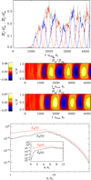 |
Fig. 3 Reference solution dynamo. Top: normalised volume averages of the squared horizontal magnetic field components, |


3.1.2 Understanding the dynamo
Defining  , and recalling that an overbar denotes a horizontal average, it can be shown that
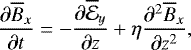 (20)
whilst
(20)
whilst
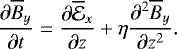 (21)
(21)
With the given boundary and initial conditions, it is straightforward to show that  for all z and t. In the absence of a significant mean flow, standard mean-field dynamo theory (e.g. Moffatt 1978) suggests that there should be a linear relationship between the components of the mean electromotive force,
  , and the components and z-derivatives of
  . To be more specific, we might expect relations of the form
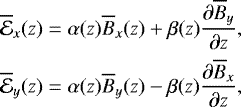 (22)
where α(z) and β(z) are scalar functions of height only. Whilst the β(z) term would dominate near the boundaries where the mean magnetic field vanishes (and the field gradient is large), we might expect the α(z) term to dominate in a non-negligible region in the vicinity of the mid-plane where the mean field gradient is relatively small. Having said that, it should be stressed that the flow that is responsible for driving this large-scale dynamo is the product of a fully non-linear magnetohydrodynamic state. Even before the large-scale magnetic field starts to grow, this flow is strongly influenced by magnetic effects. As noted by Courvoisier et al. (2009), this probably implies that the relationship between
(22)
where α(z) and β(z) are scalar functions of height only. Whilst the β(z) term would dominate near the boundaries where the mean magnetic field vanishes (and the field gradient is large), we might expect the α(z) term to dominate in a non-negligible region in the vicinity of the mid-plane where the mean field gradient is relatively small. Having said that, it should be stressed that the flow that is responsible for driving this large-scale dynamo is the product of a fully non-linear magnetohydrodynamic state. Even before the large-scale magnetic field starts to grow, this flow is strongly influenced by magnetic effects. As noted by Courvoisier et al. (2009), this probably implies that the relationship between  and
and  is more complicated than that suggested by Eq. (22). We defer detailed considerations of this question to future work, focusing here upon the form of
  and the components of the flow that are responsible for producing it.
Figure 4 shows contour plots of  and (for comparison)
  as functions of z and t, taken from a simulation that duplicates the reference solution parameters, but is evolved from a state with a weaker initial thermal perturbation. A quantitatively comparable solution is obtained, indicating that this large-scale dynamo is robust to such changes to the initial conditions. Clearly
  exhibits much stronger temporal fluctuations than
  , whilst
  is more asymmetric about the mid-plane than
  . Nevertheless, in purely qualitative terms, there are some indications of a simple temporal correlation between
  and
and  , with a similar long timescale variation apparent in both cases. This is not inconsistent with the relation suggested by Eq. (22). Although not shown here,
  and
and  evolve in a similar way.
As we have already noted, the large-scale vortex is strongly suppressed by the magnetic field. To confirm that the low wavenumber components of the flow make a negligible contribution to this large-scale dynamo, we have investigated the effects of removing the low wavenumber content from the flow before calculating  . It should be emphasised that we are not making any changes to the dynamo calculation itself; all filtering is carried out in post-processing. The upper part of Fig. 5 shows the effects of removing all Fourier modes with k∕k1 ≤ 2 before calculating
  (although not shown here, similar results are obtained for
  ). At least in qualitative terms, it is clear that this is comparable to the corresponding unfiltered
  that is shown in Fig. 4. A much more significant change is observed when modes with k∕k1 ≤ 6 are removed: this filtered
  appears to be almost antisymmetric about the mid-plane, with some propagation of activity away from the mid-plane that is not apparent in the reference solution. Intriguingly, there is a significant fraction of the domain over which this filtering process actually changes the sign of the resulting
  (compared to the corresponding unfiltered case). This sign change occurs gradually as the filtering threshold is increased from k∕k1 = 2 to 6, so there is no abrupttransition. Further increments to this filtering threshold lead to no further qualitative changes in the distribution of
  , although its amplitude obviously decreases as more components are removed from the flow.
Figure 6 shows the time-averaged values of  as a function of z, for the filtered and unfiltered cases. Clearly the first filtered case, with only the k∕k1 ≤ 2 modes removed, is quantitatively comparable to the unfiltered case, which reinforces the notion that the low wavenumber content of the flow plays no significant role in the dynamo. On the other hand, the clear quantitative differences between thetwo filtered cases indicate that components of the flow with horizontal wavenumbers in the range 3 ≤ k∕k1 ≤ 5 play a crucial role in driving this large-scale dynamo. It is worth highlighting the fact that the small-scale motions alone seem to be capable of producing a coherent, systematically varying
  with a peak value that is of comparable magnitude to the peak value of the unfiltered
  . This suggests that it may be possible for the small-scale motions alone to sustain a dynamo. Having said that, it should also be emphasised that these small-scale motions are not independent of the large-scale flows and magnetic field in the system (we stress again that all filtering is carried out in post-processing), and so the small-scale motions are almost certainly strongly influenced by the fact that a large-scale dynamo is operating. Whilst it is tempting to speculate that there may be some connection here with the near-onset dynamos of e.g. Stellmach & Hansen (2004), which rely purely on small-scale motions, we have not yet been able to demonstrate this in a conclusive manner.
Having identified the components of the flow that are responsible for driving the large-scale dynamo, we conclude this section with a brief comment on the role of the magnetic boundary conditions. Integrating Eqs. (20) and (21) over z, it is straightforward to verify that our magnetic boundary conditions (in which Bx = By = 0 at z = 0 and z = 1) allow the net horizontal flux to vary in time (cf. the near-onset study of Favier & Proctor 2013). In particular, these boundary conditions allow for the diffusive transport of magnetic flux out of the domain. Recalling that the dynamo oscillates on a timescale that is of the same order of magnitude as the ohmic decay time across the layer, it is probable that the cycle period of the dynamo reflects the rate at which horizontal magnetic flux can be ejected from the domain. Assuming that the simple mean-field ansatz of Eq. (22) is a reasonable description of  , this process would be accelerated by a positive β(z) at the boundaries (which would enhance diffusion), so we should not be surprised to find examples of this dynamo with a considerably shorter cycle period. Having said that, even a large β(z) at the boundaries can only help if the boundary conditions allow it to do so. If we were to modify the magnetic boundary conditions to the Soward–Childress (perfect conductor) conditions of Bz = ∂By∕∂z = ∂Bx∕∂z = 0 at z = 0 and z = 1, that would mean that the total horizontal flux would be invariant (initially set to zero). Under these circumstances, we have confirmed that a simulation with the reference dynamo parameters produces only a small-scale dynamo. Of course, we cannot exclude the possibility that there are regions of parameter space in which a large-scale dynamo can be excited via this large-scale vortex mechanism, with these perfectly conducting magnetic boundary conditions. However, we can say that these simulations suggest that such a configuration would be less favourable for large-scale dynamo action than the vertical conditions that we have adopted here.
As a final remark, it is worth noting that one way of circumventing the dependence of this dynamo upon the magnetic boundary conditions is to include one or more convectively stable layers into the system (Käpylä et al. 2013), which could reside eitherabove or below the convective layer. Even if perfectly conducting boundary conditions are applied, such a stable region can act as a “flux repository” for the system: if the convective layer can expel a sufficient quantity of magnetic flux into this region, the large-scale dynamo could continue to operate as described above (as is the case for run D1e in Käpylä et al. 2013). Whilst we emphasise that this is not a model for the solar dynamo, the possible importance of an underlying stable layer acting as a flux repository has also been recognised in that context. Certain solar dynamo models (e.g. Parker 1993; Tobias 1996a; MacGregor & Charbonneau 1997) rely on the assumption that the bulk of the large-scale toroidal magnetic flux in the solar interior resides in the stable layer just below the base of the convection zone. This can therefore be regarded as another example of a situation in which the addition of a stable layer can be beneficial for dynamo action.
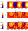 |
Fig. 4 Time and z dependence of |


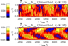 |
Fig. 5 Contours of |


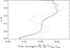 |
Fig. 6 Time-averaged |


3.2 Sensitivity to parameters
As indicated in Table 1, we have carried out a range of simulations to assess the sensitivity of the reference solution dynamo to variations in the parameters. Cases B1–8 were all initialised from our standard polytropic state, whilst cases C1–5 were initialised from the reference solution (A2). Cases D1–3 investigated the effects of increasing Ra and Ta at a fixed convective Rossby number, Ro_c. Finally, case E1 is a pseudo-Boussinesq calculation with the initial density varying linearly between 0.9 and 1.1; all other parameters (including the polytropic index) were identical to the reference solution.
When comparing dynamos at different rotation rates, it is convenient to consider the modified Rayleigh number,  . For ease of comparison with previous studies, it is worth recalling that the Ekman number, Ek, is related to the Taylor number by Ek = Ta−1∕2. So
  is equivalent to Ra Ek4∕3, which tends to be the more usual form of this parameter in the geodynamo literature. Figure 1 in Guervilly et al. (2015) suggests that
  must exceed a value of approximately 20 for the large-scale vortex instability to operate (obviously rapid rotation is also required). For the reference solution,
  , which is certainly consistent with that picture. The other point to note from Fig. 1 of Guervilly et al. (2015) is that (in the absence of a large-scale vortex instability) large-scale dynamos tend to be restricted to a small region of parameter space in which the layer is rapidly rotating (i.e. Ta > 108; equivalently, Ek < 10−4) and the convection is only weakly supercritical (typically,
  is O(10)).
Following a similar approach to that of Guervilly et al. (2015), Fig. 7 shows how the simulations that are reported in this paper compare with others in the literature. These dynamo simulations are classified according to  and Ek (the Ekman number has been used here, rather than the Taylor number, for ease of comparison with Guervilly et al. 2015). The shaded area indicates the approximate region of parameter space where the large-scale vortex instability has been observed, although the limits of this region also depend to some extent on the aspect ratio of the corresponding simulation domains. The parameter regime in the lower right part of the plot is also likely to support large-scale vortices, but numerical simulations in this regime are currently beyond the available computational resources. It should be stressed that there are many different types of convective dynamos on this plot. Some simulations are Boussinesq rather than compressible, others have perfectly conducting magnetic boundary conditions, others feature underlying and/or overlying stable layers. These model differences become particularly important at the edges of the large-scale vortex region. Focusing on the upper left corner of the shaded region, the single-layer calculation of Favier & Bushby (2013) was just outside of the large-scale vortex region and so found a small-scale dynamo. The large-scale vortex instability was, however, present in the multiple-layer model of Käpylä et al. (2013), which explains the observation of large-scale dynamo action in that case. Having said that, regardless of the details of the model, it is clear that the large-scale vortex instability seems to provide a route by which large-scale dynamos can be found in moderately supercritical, rapidly rotating convection, outside of their normal operative region of parameter space.
It is worth emphasising at this stage that not all simulations in the large-scale vortex parameter region produce large-scale dynamos. In particular, we only find small-scale dynamos at low aspect ratios (i.e. λ < 2). For λ = 1 (see cases B6, B7, and B8, which correspond to the orange diamonds in Fig. 7), this is true even at higher rotation rates where there is a greater separation in scales between the domain size and the horizontal scale of the near-onset convective motions. The failure of the large-scale dynamo in this case can probably be attributed to the fact that the large-scale vortex instability, which plays a crucial role in initialising the dynamo, is inhibited in smaller domains (see also Guervilly et al. 2015). Certainly, the large-scale vortex (measured, for example, by the rms velocity) stops growing long before the magnetic field becomes dynamically significant, which suggests that geometrical effects are limiting its growth in these low aspect ratio cases. A strong suppression of the large-scale vortex will also limit the production of motions at those intermediate scales that are responsible for sustaining the large-scale dynamo.
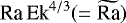
Figure 8 shows the cycle frequency, ωcyc = 2π∕τcyc (where τcyc is the cycle period), for the successful large-scale dynamos, as a function of  . To ensure somedegree of comparability across the simulations, the cycle frequency has been normalised by the ohmic decay time, τη, in each case. This choice of normalisation was motivated by the comparability of τη and τcyc for the reference solution (and reflects the important role played by diffusive processes in the underlying dynamo mechanism). Case E1 has been excluded from this plot because it has not been evolved for long enough to produce an accurate determination of the cycle period, for reasons that are discussed below. Across the other simulations, a clear trend is observed when moving closer to convective onset: cycle frequencies tend to decrease with decreasing
  . So, as we move closer to onset, the dynamo cycles become longer (cf. Calkins et al. 2016, who found a similar result in a related quasi-geostrophic dynamo model). In fact, this trend accounts for the uncertainty regarding whether C5 is a large-scale dynamo. If it were a large-scale dynamo, it would have an extremely long cycle period, but we were unable to run this calculation for long enough to establish whether or not this was the case. At higher convective driving, modulation effects (as discussed in the next section) make it more difficult to determine cycle frequencies in some cases. However, it is clear that there is a greater degree of variability in the cycle frequencies at higher values of
  . For example, despite the rather similar values of
  , the normalised cycle frequencies for cases D2 and B3a differ by more than a factor of two. This suggests some dependence of the cycle frequency upon some of the other parameters in the system besides
  (a possible candidate is the convective Rossby number, Ro_c, which is fixed in cases D1–3, but is free to vary in cases B1–8). These differences aside, although there is not a single best fit curve, there is still a clear tend of increasing cycle frequencies with increasing levels of convective driving. The shortest period dynamos have a cycle period that is about 10% of τη. Even in these cases, the cycle periods are still long enough that diffusive effects are probably playing a significant role.
Whilst these large-scale dynamos do exhibit weak departures from symmetry about the mid-plane, there are no obvious suggestions that the stratification of the fluid is playing a major role in the operation of the dynamo. Indeed, as illustrated in Fig. 9, our quasi-Boussinesq case (E1) produces much the same dynamo solution as the reference case. Only a relatively short time-series is shown in this figure (in this quasi-Boussinesq regime, the time-step constraints that are associated with acoustic modes make long calculations prohibitively expensive), but it is clear that the behaviour of this solution is qualitatively similar to that of the corresponding stages of the reference solution, so it is very unlikely that this large-scale dynamo willnot persist. In such cases, it is clearly more efficient to consider a proper Boussinesq model; whilst not shown here, we have confirmed that a Boussinesq calculation (using the code described by Cattaneo et al. 2003) can produce a similar large-scale dynamo with the reference solution parameter values. Due to the Boussinesq symmetries,  and
and  are anti-symmetric about the mid-plane, but the mean horizontal magnetic fields are again symmetric. The only significant change due to the reduction in the level of stratification is in the cycle period. The Boussinesq run suggests a cycle period (normalised by the convective turnover time) that is approximately twice that of the reference solution. Whilst it is still evolving, the quasi-Boussinesq case E1 appears to be consistent with this, with a longer cycle period compared to that seen in the corresponding plots in Fig. 3. The ohmic decay time in case E1 is approximately 2350 turnover times, which is similar to that of the reference solution, so this longer cycle period is not simply a function of normalisation. Having said that, as indicated by Fig. 8, small changes in the convective driving can lead to large changes in the cycle period in the vicinity of the reference solution, so this discrepancy between thecycle periods is probably not that significant. If anything, it is more remarkable that this seems to be the only significant effect on the dynamo that can be attributed to a reduction in the stratification of the layer.
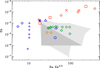 |
Fig. 7 Ek plotted against |
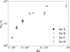 |
Fig. 8 Cycle frequency, ωcyc, of large-scaledynamo simulations plotted against |

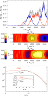 |
Fig. 9 As Fig. 3, but here for the weakly stratified (quasi-Boussinesq) case, E1. The time-series here is relatively short because the numerical time-step constraints make longer runs very difficult to carry out. |
3.3 Temporal modulation
As noted in Table 1, there are a number of cases in which the large-scale dynamo activity is described as“intermittent”. Recalling that the critical Rayleigh number for the onset of convection is Ra crit = 6.006 × 10⁶ for this set of parameters, these cases are considerably more supercritical (in terms of their convective driving) than the reference solution. For cases B3a and B3b, Ra ≈ 6.7 Racrit, whilst Ra ≈ 8.3 Racrit for case B4 and Ra ≈ 10.0 Racrit for case B5. In each case, the large-scale vortex instability leads to vigorous convective flows.
Even in the case of the large-scale dynamo in the reference solution, there is some evidence of modulation in the mean magnetic field, with the peak horizontally averaged magnetic field varying noticeably from one cycle to the next. Small increases in the Rayleigh number amplify this effect. This is illustrated in Fig. 10, which shows the large-scale dynamo for case B2 (Ra = 3 × 10⁷ ≈ 5.0 Racrit). In this simulation, the depth-averaged mean squared horizontal magnetic field (at ~ 2750 convective turnover times) peaks at approximately 25% of the squared equipartition field strength. The weakest cycles peak at approximately 5% of this equipartition value. Some fluctuations are visible in both the Urms(t) and Brms(t) time-series, although these are fairly modest, particularly in the case of Urms(t).
Moving to higher Rayleigh numbers, we see much more dramatic modulation. Figure 11 shows the evolution of the large-scale dynamo for case B3a. Whilst the large-scale dynamo is generally weaker (in terms of its equipartition value) than similar dynamos at lower Rayleigh number, it is still possible to identify well-defined oscillations in the mean horizontal magnetic field. However, the modulation is now extremely pronounced, with “active phases” of large-scale cyclic behaviour punctuated by periods of negligible large-scale activity (during which the generated magnetic field is predominantly small scale). At even higher Rayleigh numbers, this modulation pattern reverses, with bursts of large-scale activity surrounded by long periods of relative inactivity (see Fig. 12). For case B3a, large-scale activity cycles can be seen over approximately two-thirds of the time-series (mostly active phases, but with recurrent periods of inactivity). This behaviour becomes increasingly intermittent at larger values of the Rayleigh number: B4 is active for about one-third of the time series, whereas B5 is active for approximately one-quarter of the time.
Certainly in the case of B3a, this modulation behaviour is rather reminiscent of that observed in the solar cycle, where extended phases of reduced magnetic activity (such as the Maunder Minimum, see e.g. Eddy 1976), often referred to as grand minima, have been a recurrent feature of the activity pattern over at least the last 10 000 years (see e.g. McCracken et al. 2013). We stress again that we do not claim to be modelling the solar dynamo in this paper. Nevertheless, there may be some similarities between the modulation mechanism in these simulations with that of the Sun. As can clearly be seen in Figs. 11 and 12, the rms velocity in these simulations tends to increase during grand minima. This corresponds to the re-emergence of the large-scale vortex instability. During these inactive phases, the magnetic field is no longer strong enough to suppress this large-scale flow (which can be seen in the time-series of the rms magnetic field), so it can again grow. It then becomes temporarily suppressed again once the magnetic field reaches dynamically significant levels. A number of authors have proposed mean-field models of the solar dynamo in which long-term modulation arises as the result of the magnetic field inhibiting the large-scale differential rotation (see e.g. Tobias 1996b; Brooke et al. 2002; Bushby 2006). In these models, the occurrence of grand minima depended upon there being a separation in timescales between viscous and magnetic diffusion, sothat the perturbations to the flow velocity relaxed over a much longer timescale than the period of oscillation of the dynamo. There is a similar separation in timescales in these modulated convective dynamo simulations, with the large-scale vortex growing on a much longer timescale than the cycle period of the large-scale dynamos. The exchange of energy between the magnetic field and the flow can therefore give rise to this modulation behaviour.
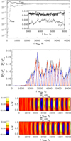 |
Fig. 10 Dynamo evolution for Case B2. Top: time evolution of the rms velocity and magnetic field (the inset highlights the modulation during the non-linear phase). Middle: volume-averaged squared horizontal fields, |


4 Conclusions and discussion
One of the great challenges for dynamo theorists is to explain the origin of large-scale astrophysical magnetic fields. As anticipated from theory, helically forced turbulence in an electrically conducting fluid can drive a large-scale dynamo in a Cartesian domain (Brandenburg 2001). Such idealised flows can never be realised in nature, although the effects of rotation are believed to give rise to helical convective motions in many astrophysical bodies, so similar large-scale dynamos might be expected in such cases. However, the dynamo properties of rapidly rotating convection appear to be rather subtle. Near-onset rapidly rotating convection can drive a large-scale dynamo in a Cartesian domain (Childress & Soward 1972), but unless there is an imposed shear (which tends to promote large-scale dynamo action, see e.g. Käpylä et al. 2008; Hughes & Proctor 2009) dynamos tend to be small-scale in the more turbulent regime that is relevant for astrophysics.
Previous work (Käpylä et al. 2013; Masada & Sano 2014a,b) has demonstrated that it is possible to find a large-scale dynamo in moderately turbulent, rapidly rotating convection in a Cartesian domain (without shear). These simulations are in a parameter regime in which the large-scale vortex instability can operate. Building on this previous work, we have carried out a detailed analysis of the underlying dynamo mechanism and have demonstrated that the large-scale dynamo is driven by the components of the flow with a horizontal wavenumber in the range 3 ≤ k∕k1 ≤ 5. In particular, this confirms that the large-scale vortex itself (i.e. the k = k1 mode, which becomes strongly damped) does not play a direct role in sustaining the dynamo. Having said that, the structure of the flow at the driving scales is still influenced (to some extent, at least) by the tendency for the large-scale vortex instability to transfer energy to larger scales. So, even though the large-scale vortex itself is damped, the effects of the underlying instability should not be discounted. In particular the initialisation of the large-scale dynamo in this parameter regime may well depend upon there being an efficient large-scale vortex instability in the first place. As a prelude to a possible benchmarking exercise, we have verified that this dynamo can be reproduced by three different codes, all of which produce quantitatively comparable solutions in the non-linear regime.
Provided that the magnetic boundary conditions (which appear to be very important in this context) allow magnetic flux to escape from the domain, we have shown that this large-scale dynamo is robust to moderate changes in the parameters. The dynamo appears to be largely insensitive to the level of stratification within the domain, although the calculations that we have carried out do suggest that large-scale dynamos in more weakly stratified domains tend to have longer cycle periods. Moving towards convective onset, the form of the dynamo remains largely the same, although the cycle period of the large-scale dynamo increases (very dramatically at the lowest Rayleigh numbers). As the level of convective driving is increased, the cycle period decreases, and the cycle becomes increasingly modulated. At moderate Rayleigh numbers, this modulation is almost solar-like, with active phases punctuated by inactive grand minima. At higher driving, the large-scale dynamo becomes increasingly intermittent. The modulation is driven by an exchange of energy between the magnetic field and the flow.
Future investigations in this field will focus on even more turbulent regimes at higher Rayleigh numbers, exploring broad ranges of magnetic and thermal Prandtl numbers and rotation rates. The dynamo mechanism could also be analysed from the perspective of mean-field dynamo theory. We have seen that there is a positive correlation between the components of the mean horizontal magnetic field and the mean horizontal electromotive force, just as expected for an α2 dynamo located in the northern hemisphere of a rotating star, but more could be done to clarify this. It would also be worthwhile to investigate possible connections between these moderately turbulent large-scale dynamos and the near-onset Boussinesq dynamos. We have shown that vertical field boundary conditions seem to promote this large-scale dynamo, but this does not rule outthe possibility that a similar dynamo could operate in a turbulent regime with the horizontal field boundary conditions adopted in most Boussinesq studies. Finally, there is the intriguing question of the extent to which these Cartesian dynamos are of relevance to particular astrophysical bodies. Is it possible to find analogous dynamos in a sphere or spherical shell? Obviously the cycle periods of these large-scale dynamos are too long to be of direct relevance to solar-type dynamos, but we can speculate that there may be some possible application to planetary dynamos where, at least in the case of the Earth, we know that there are polarity reversals over long timescales.
Acknowledgements
We would welcome any interest from the dynamo community in the benchmark exercise that is proposed in Appendix A. This work has been supported in part by the National Science Foundation (grant AST1615100), the Research Council of Norway under the FRINATEK (grant 231444), the Swedish Research Council (grant 621-2011-5076), the University of Colorado through its support of the George Ellery Hale visiting faculty appointment (AB), the Academy of Finland (grant 272157) to the ReSoLVE Centre of Excellence (PJK, MJK), and the UK Natural Environment Research Council (grant NE/M017893/1, CG). Some of the simulations were performed using the supercomputers hosted by CSC – IT Center for Science Ltd. in Espoo, Finland, which is administered by the Finnish Ministry of Education. Much of this work has made use of the facilities of N8 HPC Centre of Excellence, provided and funded by the N8 consortium and EPSRC (Grant No. EP/K000225/1). The Centre is co-ordinated by the Universities of Leeds and Manchester. PB would also like to acknowledge a useful discussion with Michael Proctor that helped to clarify the nature of the underlying dynamo mechanism. We would also like to thank the referee for the helpful comments and suggestions.
Appendix A: A possible dynamo benchmark
This appendix contains further details on the quantitative comparison that has been carried out between the three codes that are described in Sect. 2.4. The aim here is to assess whether or not this large-scale dynamo solution could form the basis for a community-wide non-linear dynamo benchmark. We choose to present the details here to encourage other researchers with similar codes to try this calculation. If there is sufficient enthusiasm from the community to carry out a detailed benchmark study, we would agree on a common set of initial conditions and carry out a detailed analysis of the early evolution of the system (e.g. comparing the mean growth rate of Urms(t) during the large-scale vortex phase) and of the final non-linear state. Whilst this solution is relatively complicated, we would (at the very least) expect different codes to produce quantitatively comparable statistics. Here, we focus upon the simpler question of whether or not the final non-linear solution is robust to small changes in the initial conditions, confirming that three independent codes can produce quantitatively comparable non-linear dynamos.
Details of the benchmark simulations.
Fixing λ = 2, Pr = Pm = 1, and Ta = 5 × 10⁸, it was first confirmed that all three codes agree on the critical Rayleigh number, Ra crit = 6.006 × 10⁶, with exponentially growing (decaying) solutions being obtained for values of Ra that are fractionally above (below) this value. Once this agreement was confirmed, non-linear dynamo runs were carried out for the reference solution value of Ra = 2.4 × 10⁷ (see the upper three rows of Table 1). As has already been described, this reference solution exhibits highly non-trivial behaviour in which the initial convective instability is subject to a secondary hydrodynamical instability (corresponding to the large-scale vortex). The resulting flow then drives a non-linear large-scale dynamo in which the total magnetic and kinetic energies are in a state of near-equipartition. This solution is therefore an excellent test of all aspects of any compressible Cartesian MHD code. Although they were all evolved from the same initial polytropic state, random initial perturbations were applied. Some quantitative differences between the codes are therefore to be expected during the early stages of evolution.If, however, it is possible to confirm that all of the codes converge upon the same non-linear dynamo, then this comparison can be deemed successful.
Figures A.1–A.4 show the evolution of this system for each of the three codes. Figure A.1 shows the time evolution of the rms velocity and magnetic field. The time- and z-dependence of the mean horizontal magnetic field components is illustrated in Fig. A.2, whilst Fig. A.3 shows the corresponding vertically averaged values. Finally, Fig. A.4 shows the mid-layer kinetic and magnetic energy spectra at the end of the three runs. It is immediately apparent that all three codes are producing quantitatively comparable non-linear dynamos. There are similar pronounced peaks at k = 0 in the magnetic energy spectra, whilst the kinetic energy spectra all have broad peaks at around k∕k1 = 7–9. The peak amplitudes of the large-scale horizontal magnetic field components show similar levels of agreement (as indicated by Fig. A.3). Table A.1 shows the time-averaged values of urms and brms, respectively the rms velocity and magnetic field, from the non-linear phase of the dynamo. It is clear that there is quantitative comparability for both of these quantities across the three codes. Whilst there is some variability in terms of the measured cycle periods (970, 1050, and 1060 convective turnover times), it should be noted that there is some intrinsic variation in the cycle duration as the dynamo progresses. This is one of the main contributors to the error bars in Fig. 8, and the variation across the three codes could simply reflect this variability. This variability in the cycle period may complicate a future benchmarking exercise, but this can probably be addressed satisfactorily by running longer calculations to average the cycle period over more cycles.
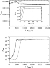 |
Fig. A.1 Root mean square velocity (top) and magnetic field (bottom) for Code 1 (solid line), Code 2 (dashed line), and Code 3 (dash-dotted line). The inset in the upper plot shows the early time behaviour, highlighting the different initial conditions that have been used. |
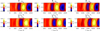 |
Fig. A.2 Horizontally averaged horizontal magnetic fields (normalised by the equipartition field strength) as functions of z and time forCode 1 (left), Code 2 (middle), and Code 3 (right). The time-axes for Codes 2 and 3 have been shifted by 420 turnover times and 480 turnover times, respectively, for ease of comparison with Code 1. |
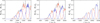 |
Fig. A.3 Volume-averaged horizontal (squared) magnetic fields, |


 |
Fig. A.4 Typical power spectra of velocity (black lines) and magnetic field (red lines) from the middle of the convective layer for Code 1 (left), Code 2 (middle), and Code 3 (right). In each case, the inset shows the smallest wavenumbers to illustrate that the magnetic field peaks at k = 0. All spectra quantities are normalised by the average kinetic energy at zm during the non-linear phase. |
We should also note some other differences between the three cases. As shown by Fig. A.1, the initial large-scale vortex growth phase is longer in Code 3 (with a lower growth rate) than it is in the other two codes. This can be probably attributed to differences in the initial conditions: the initial rms velocity starts from a much lower level in the case of Code 3, which apparently delays the onset of the large-scale vortex instability. It is also worth noting that the seed magnetic field is weaker in Code 3 than it is in the others, so it takes longer to grow to a level where it is able to influence the flow. This dependence upon the strength of the seed field clearly indicates that it is the Lorentz force that is eventually suppressing the large-scale vortex instability rather than a geometrical constraint due to the finite box size. Further differences can be seen in Figs. A.2 and A.3, where the large-scale dynamo emerges at different times for the different codes. Again, this can be explained by differences in the initial conditions. The important point to note is that this large-scale dynamo is robust to small variations in the initial configuration.
This non-linear dynamo solution is therefore an excellent benchmark candidate.
References
- Brandenburg, A. 2001, ApJ, 550, 824 [NASA ADS] [CrossRef] [Google Scholar]
- Brandenburg, A., Saar, S. H., & Turpin, C. R. 1998, ApJ, 498, L51 [NASA ADS] [CrossRef] [Google Scholar]
- Brooke, J., Moss, D., & Phillips, A. 2002, A&A, 395, 1013 [NASA ADS] [CrossRef] [EDP Sciences] [Google Scholar]
- Bushby, P. J. 2006, MNRAS, 371, 772 [Google Scholar]
- Calkins, M. A., Julien, K., Tobias, S. M., & Aurnou, J. M. 2015, J. Fluid Mech., 780, 143 [NASA ADS] [CrossRef] [Google Scholar]
- Calkins, M. A., Julien, K., Tobias, S. M., Aurnou, J. M., & Marti, P. 2016, Phys. Rev. E, 93, 023115 [NASA ADS] [CrossRef] [Google Scholar]
- Cattaneo, F., & Hughes, D. W. 2006, J. Fluid Mech., 553, 401 [NASA ADS] [CrossRef] [Google Scholar]
- Cattaneo, F., Emonet, T., & Weiss, N. 2003, ApJ, 588, 1183 [NASA ADS] [CrossRef] [MathSciNet] [Google Scholar]
- Chan, K. L. 2007, Astron. Nachr., 328, 1059 [NASA ADS] [CrossRef] [Google Scholar]
- Chan, K. L., & Mayr, H. G. 2013, Earth Planet. Sci. Lett., 371, 212 [NASA ADS] [CrossRef] [Google Scholar]
- Chandrasekhar, S. 1961, Hydrodynamic and hydromagnetic stability (Oxford University Press) [Google Scholar]
- Childress, S., & Soward, A. M. 1972, Phys. Rev. Lett., 29, 837 [NASA ADS] [CrossRef] [Google Scholar]
- Christensen, U. R., Aubert, J., Cardin, P., et al. 2001, Phys. Earth Planet. Int., 128, 25 [NASA ADS] [CrossRef] [Google Scholar]
- Clarke, D. A. 1996, ApJ, 457, 291 [NASA ADS] [CrossRef] [Google Scholar]
- Colella, P., & Woodward, P. R. 1984, J. Comp. Phys., 54, 174 [Google Scholar]
- Courvoisier, A., Hughes, D. W., & Proctor, M. R. E. 2009, Roy. Soc. London Philos. Trans. Ser. A, 466, 583 [NASA ADS] [CrossRef] [Google Scholar]
- Dobler, W., Stix, M., & Brandenburg, A. 2006, ApJ, 638, 336 [NASA ADS] [CrossRef] [Google Scholar]
- Eddy, J. A. 1976, Science, 192, 1189 [NASA ADS] [CrossRef] [PubMed] [Google Scholar]
- Evans, C. R., & Hawley, J. F. 1988, ApJ, 332, 659 [Google Scholar]
- Fautrelle, Y., & Childress, S. 1982, Geophys. Astrophys. Fluid Dyn., 22, 235 [NASA ADS] [CrossRef] [Google Scholar]
- Favier, B., & Bushby, P. J. 2012, J. Fluid Mech., 690, 262 [NASA ADS] [CrossRef] [Google Scholar]
- Favier, B., & Bushby, P. J. 2013, J. Fluid Mech., 723, 529 [NASA ADS] [CrossRef] [Google Scholar]
- Favier, B., & Proctor, M. R. E. 2013, Phys. Rev. E, 88, 053011 [NASA ADS] [CrossRef] [Google Scholar]
- Favier, B., Silvers, L. J., & Proctor, M. R. E. 2014, Phys. Fluids, 26, 096605 [NASA ADS] [CrossRef] [Google Scholar]
- Guervilly, C., Hughes, D. W., & Jones, C. A. 2014, J. Fluid Mech., 758, 407 [NASA ADS] [CrossRef] [Google Scholar]
- Guervilly, C., Hughes, D. W., & Jones, C. A. 2015, Phys. Rev. E, 91, 041001 [NASA ADS] [CrossRef] [Google Scholar]
- Hughes, D. W., & Proctor, M. R. E. 2009, Phys. Rev. Lett., 102, 044501 [NASA ADS] [CrossRef] [Google Scholar]
- Jones, C. A. 2011, Ann. Rev. Fluid Mech., 43, 583 [NASA ADS] [CrossRef] [Google Scholar]
- Jones, C. A., & Roberts, P. H. 2000, J. Fluid Mech., 404, 311 [NASA ADS] [CrossRef] [Google Scholar]
- Jones, C. A., Boronski, P., Brun, A. S., et al. 2011, Icarus, 216, 120 [NASA ADS] [CrossRef] [Google Scholar]
- Julien, K., Rubio, A. M., Grooms, I., & Knobloch, E. 2012, Geophys. Astrophys. Fluid Dyn., 106, 392 [NASA ADS] [CrossRef] [Google Scholar]
- Käpylä, P. J., Korpi, M. J., & Brandenburg, A. 2008, A&A, 491, 353 [NASA ADS] [CrossRef] [EDP Sciences] [Google Scholar]
- Käpylä, P. J., Korpi, M. J., & Brandenburg, A. 2009, ApJ, 697, 1153 [NASA ADS] [CrossRef] [Google Scholar]
- Käpylä, P. J., Mantere, M. J., & Hackman, T. 2011, ApJ, 742, 34 [NASA ADS] [CrossRef] [Google Scholar]
- Käpylä, P. J., Mantere, M. J., & Brandenburg, A. 2013, Geophys. Astrophys. Fluid Dyn., 107, 244 [Google Scholar]
- Kunnen, R. P. J., Ostilla-Mónico, R., van der Poel, E. P., Verzicco, R., & Lohse, D. 2016, J. Fluid Mech., 799, 413 [NASA ADS] [CrossRef] [Google Scholar]
- MacGregor, K. B., & Charbonneau, P. 1997, ApJ, 486, 484 [NASA ADS] [CrossRef] [Google Scholar]
- Mantere, M. J., Käpylä, P. J., & Hackman, T. 2011, Astron. Nachr., 332, 876 [NASA ADS] [CrossRef] [Google Scholar]
- Marti, P., Schaeffer, N., Hollerbach, R., et al. 2014, Geophys. J. Int., 197, 119 [NASA ADS] [CrossRef] [Google Scholar]
- Masada, Y., & Sano, T. 2014a, PASJ, 66, 2 [CrossRef] [Google Scholar]
- Masada, Y., & Sano, T. 2014b, ApJ, 794, L6 [NASA ADS] [CrossRef] [Google Scholar]
- Masada, Y., & Sano, T. 2016, ApJ, 822, L22 [NASA ADS] [CrossRef] [Google Scholar]
- Matthews, P. C., Proctor, M. R. E., & Weiss, N. O. 1995, J. Fluid Mech., 305, 281 [NASA ADS] [CrossRef] [Google Scholar]
- McCracken, K., Beer, J., Steinhilber, F., & Abreu, J. 2013, Space Sci. Rev., 176, 59 [NASA ADS] [CrossRef] [Google Scholar]
- Meneguzzi, M., & Pouquet, A. 1989, J. Fluid Mech., 205, 297 [NASA ADS] [CrossRef] [Google Scholar]
- Mizerski, K. A., & Tobias, S. M. 2013, Geophys. Astrophys. Fluid Dyn., 107, 218 [NASA ADS] [CrossRef] [Google Scholar]
- Moffatt, H. K. 1978, Magnetic field generation in electrically conducting fluids (Cambridge University Press) [Google Scholar]
- Parker, E. N. 1993, ApJ, 408, 707 [Google Scholar]
- Rotvig, J., & Jones, C. A. 2002, Phys. Rev. E, 66, 056308 [NASA ADS] [CrossRef] [MathSciNet] [Google Scholar]
- Sano, T., Inutsuka, S., & Miyama, S. M. 1999, in Numerical Astrophysics, eds. S. M. Miyama, K. Tomisaka, & T. Hanawa, Astrophys. Space Sci. Lib., 240, 383 [NASA ADS] [CrossRef] [Google Scholar]
- Soward, A. M. 1974, Roy. Soc. London Philos. Trans. Ser. A, 275, 611 [NASA ADS] [CrossRef] [Google Scholar]
- St. Pierre, M. G. 1993, in Solar and Planetary Dynamos, eds. M. R. E. Proctor, P. C. Matthews, & A. M. Rucklidge, 295 [Google Scholar]
- Stellmach, S., & Hansen, U. 2004, Phys. Rev. E, 70, 056312 [NASA ADS] [CrossRef] [Google Scholar]
- Stellmach, S., Lischper, M., Julien, K., et al. 2014, Phys. Rev. Lett., 113, 254501 [NASA ADS] [CrossRef] [Google Scholar]
- Stix, M. 2002, The Sun: an introduction (Springer) [Google Scholar]
- Stone, J. M., & Norman, M. L. 1992, ApJS, 80, 791 [Google Scholar]
- Tilgner, A. 2014, Phys. Rev. E, 90, 013004 [NASA ADS] [CrossRef] [Google Scholar]
- Tobias, S. M. 1996a, ApJ, 467, 870 [NASA ADS] [CrossRef] [Google Scholar]
- Tobias, S. M. 1996b, A&A, 307, L21 [NASA ADS] [Google Scholar]
- Tobias, S. M., Cattaneo, F., & Brummell, N. H. 2011, ApJ, 728, 153 [NASA ADS] [CrossRef] [Google Scholar]
- van Leer B. 1979, J. Comp. Phys., 32, 101 [NASA ADS] [CrossRef] [Google Scholar]
- Williamson, J. H. 1980, J. Comp. Phys., 35, 48 [NASA ADS] [CrossRef] [Google Scholar]
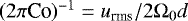 is equivalent to the standard Rossby number, based on the layer depth and the rms velocity. We use Co here so as not to confuse this quantity with the convective Rossby number, Ro_c.
All Tables
All Figures
|
Fig. 1 Time evolution of Urms(t) and Brms(t) for the reference solution. Time has been normalised by the inverse convective turnover time in the final non-linear state. |
| In the text | |
|
Fig. 2 Early stages of the reference solution. Mid-layer temperature distributions (at zm) at times turmskf = 3.4 (top) and turmskf = 362.0 (middle), plotted as functions of x and y. In each plot, the mid-layer temperature is normalised by its mean value (horizontally averaged), with the contours showing the deviations from the mean. Bottom: mid-layer kinetic energy spectra at the same times, normalised by the average kinetic energy at zm at each time. Here k is the horizontal wavenumber (in the x direction), whilst k1 = 2π∕λ is the fundamental mode. The inset highlights the low wavenumber behaviour, using a non-logarithmic abscissa to include k∕k1 = 0. |
| In the text | |
|
Fig. 3 Reference solution dynamo. Top: normalised volume averages of the squared horizontal magnetic field components, |
| In the text | |
|
Fig. 4 Time and z dependence of |
| In the text | |
|
Fig. 5 Contours of |
| In the text | |
|
Fig. 6 Time-averaged |
| In the text | |
|
Fig. 7 Ek plotted against |
| In the text | |
|
Fig. 8 Cycle frequency, ωcyc, of large-scaledynamo simulations plotted against |
| In the text | |
|
Fig. 9 As Fig. 3, but here for the weakly stratified (quasi-Boussinesq) case, E1. The time-series here is relatively short because the numerical time-step constraints make longer runs very difficult to carry out. |
| In the text | |
|
Fig. 10 Dynamo evolution for Case B2. Top: time evolution of the rms velocity and magnetic field (the inset highlights the modulation during the non-linear phase). Middle: volume-averaged squared horizontal fields, |
| In the text | |
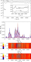 |
Fig. 11 As Fig. 10, but here for Case B3a. |
| In the text | |
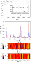 |
Fig. 12 As Fig. 10, but here for Case B4. |
| In the text | |
|
Fig. A.1 Root mean square velocity (top) and magnetic field (bottom) for Code 1 (solid line), Code 2 (dashed line), and Code 3 (dash-dotted line). The inset in the upper plot shows the early time behaviour, highlighting the different initial conditions that have been used. |
| In the text | |
|
Fig. A.2 Horizontally averaged horizontal magnetic fields (normalised by the equipartition field strength) as functions of z and time forCode 1 (left), Code 2 (middle), and Code 3 (right). The time-axes for Codes 2 and 3 have been shifted by 420 turnover times and 480 turnover times, respectively, for ease of comparison with Code 1. |
| In the text | |
|
Fig. A.3 Volume-averaged horizontal (squared) magnetic fields, |
| In the text | |
|
Fig. A.4 Typical power spectra of velocity (black lines) and magnetic field (red lines) from the middle of the convective layer for Code 1 (left), Code 2 (middle), and Code 3 (right). In each case, the inset shows the smallest wavenumbers to illustrate that the magnetic field peaks at k = 0. All spectra quantities are normalised by the average kinetic energy at zm during the non-linear phase. |
| In the text | |
Current usage metrics show cumulative count of Article Views (full-text article views including HTML views, PDF and ePub downloads, according to the available data) and Abstracts Views on Vision4Press platform.
Data correspond to usage on the plateform after 2015. The current usage metrics is available 48-96 hours after online publication and is updated daily on week days.
Initial download of the metrics may take a while.